This paper was converted on www.awesomepapers.org from LaTeX by an anonymous user.
Want to know more? Visit the Converter page.

Communication Efficient Distributed Learning for
Kernelized Contextual Bandits

\nameChuanhao Li \email[email protected]
\addrDepartment of Computer Science
University of Virginia
Charlottesville, VA 22903, USA
\AND\nameHuazheng Wang \email[email protected]
\addrSchool of Electrical Engineering and Computer Science
Oregon State University
Princeton, NJ 08544, USA
\AND\nameMengdi Wang \email[email protected]
\addrDepartment of Electrical and Computer Engineering
Princeton University
Princeton, NJ 08544, USA
\AND\nameHongning Wang \email[email protected]
\addrDepartment of Computer Science
University of Virginia
Charlottesville, VA 22903, USA
Abstract

We tackle the communication efficiency challenge of learning kernelized contextual bandits in a distributed setting. Despite the recent advances in communication-efficient distributed bandit learning, existing solutions are restricted to simple models like multi-armed bandits and linear bandits, which hamper their practical utility. In this paper, instead of assuming the existence of a linear reward mapping from the features to the expected rewards, we consider non-linear reward mappings, by letting agents collaboratively search in a reproducing kernel Hilbert space (RKHS). This introduces significant challenges in communication efficiency as distributed kernel learning requires the transfer of raw data, leading to a communication cost that grows linearly w.r.t. time horizon TT. We addresses this issue by equipping all agents to communicate via a common Nyström embedding that gets updated adaptively as more data points are collected. We rigorously proved that our algorithm can attain sub-linear rate in both regret and communication cost.

Keywords: kernelized contextual bandit, distributed learning, communication efficiency

1 Introduction

Contextual bandit algorithms have been widely used for a variety of real-world applications, including recommender systems (Li et al., 2010a), display advertisement (Li et al., 2010b) and clinical trials (Durand et al., 2018). While most existing bandit solutions assume a centralized setting (i.e., all the data reside in and all the actions are taken by a central server), there is increasing research effort on distributed bandit learning lately (Wang et al., 2019; Dubey and Pentland, 2020; Shi and Shen, 2021; Huang et al., 2021; Li and Wang, 2022), where NN clients, under the coordination of a central server, collaborate to minimize the overall cumulative regret incurred over a finite time horizon TT. In many distributed application scenarios, communication is the main bottleneck, e.g., communication in a network of mobile devices can be slower than local computation by several orders of magnitude (Huang et al., 2013). Therefore, it is vital for distributed bandit learning algorithms to attain sub-linear rate (w.r.t. time horizon TT) in both cumulative regret and communication cost.

However, prior works in this line of research are restricted to linear models (Wang et al., 2019), which could oversimplify the problem and thus leads to inferior performance in practice. In centralized setting, kernelized bandit algorithms, e.g., KernelUCB (Valko et al., 2013) and IGP-UCB (Chowdhury and Gopalan, 2017), are proposed to address this issue by modeling the unknown reward mapping as a non-parametric function lying in a reproducing kernel Hilbert space (RKHS), i.e., the expected reward is linear w.r.t. an action feature map of possibly infinite dimensions. Despite the strong modeling capability of kernel method, collaborative exploration in the RKHS gives rise to additional challenges in designing a communication efficient bandit algorithm. Specifically, unlike distributed linear bandit where the clients can simply communicate the d×dd\times d sufficient statistics (Wang et al., 2019), where dd is the dimension of the input feature vector, the joint kernelized estimation of the unknown reward function requires communicating either 1) the p×pp\times p sufficient statistics in the RKHS, where pp is the dimension of the RKHS that is possibly infinite, or 2) the set of input feature vectors that grows linearly w.r.t. TT. Neither of them is practical due to the huge communication cost.

In this paper, we propose the first communication efficient algorithm for distributed kernel bandits, which tackles the aforementioned challenge via a low-rank approximation of the empirical kernel matrix. In particular, we extended the Nyström method (Nyström, 1930) to distributed learning for kernelized contextual bandits. In this solution, all clients first project their local data to a finite RKHS spanned by a common dictionary, i.e., a small subset of the original dataset, and then they only need to communicate the embedded statistics for collaborative exploration. To ensure effective regret reduction after each communication round, as well as ensuring the dictionary remains representative for the entire distributed dataset throughout the learning process, the frequency of dictionary update and synchronization of embedded statistics is controlled by measuring the amount of new information each client has gained since last communication. We rigorously prove that the proposed algorithm incurs an O(N2γNT3)O(N^{2}\gamma_{NT}^{3}) communication cost, where γNT\gamma_{NT} is the maximum information gain that is known to be O(log(NT))O\bigl{(}\log(NT)\bigr{)} for kernels with exponentially decaying eigenvalues, which includes the most commonly used Gaussian kernel, while attaining the optimal O(NTγNT)O(\sqrt{NT}\gamma_{NT}) cumulative regret.

2 Related Works

To balance exploration and exploitation in stochastic linear contextual bandits, LinUCB algorithm (Li et al., 2010a; Abbasi-Yadkori et al., 2011) is commonly used, which selects arm optimistically w.r.t. a constructed confidence set on the unknown linear reward function. By using kernels and Gaussian processes, studies in Srinivas et al. (2009); Valko et al. (2013); Chowdhury and Gopalan (2017) further extend UCB algorithms to non-parametric reward functions in RKHS, i.e., the feature map associated with each arm is possibly infinite.

Recent years have witnessed increasing research efforts in distributed bandit learning, i.e., multiple agents collaborate in pure exploration Hillel et al. (2013); Tao et al. (2019); Du et al. (2021), or regret minimization Shi and Shen (2021); Wang et al. (2019); Li and Wang (2022). They mainly differ in the relations of learning problems solved by the agents (i.e., homogeneous vs., heterogeneous) and the type of communication network (i.e., peer-to-peer (P2P) vs., star-shaped). Most of these works assume linear reward functions, and the clients communicate by transferring the O(d2)O(d^{2}) sufficient statistics. Korda et al. Korda et al. (2016) considered a peer-to-peer (P2P) communication network and assumed that the clients form clusters, i.e., each cluster is associated with a unique bandit problem. Huang et al. Huang et al. (2021) considered a star-shaped communication network as in our paper, but their proposed phase-based elimination algorithm only works in the fixed arm set setting. The closest works to ours are (Wang et al., 2019; Dubey and Pentland, 2020; Li and Wang, 2022), which proposed event-triggered communication protocols to obtain sub-linear communication cost over time for distributed linear bandits with a time-varying arm set. In comparison, distributed kernelized contextual bandits still remain under-explored. The only existing work in this direction (Dubey et al., 2020) considered heterogeneous agents, where each agent is associated with an additional feature describing the task similarity between agents. However, they assumed a local communication setting, where the agent immediately shares the new raw data point to its neighbors after each interaction, and thus the communication cost is still linear over time.

Another closely related line of works is kernelized bandits with approximation, where Nyström method is adopted to improve computation efficiency in a centralized setting. Calandriello et al. Calandriello et al. (2019) proposed an algorithm named BKB, which uses Ridge Leverage Score sampling (RLS) to re-sample a new dictionary from the updated dataset after each interaction with the environment. A recent work by Zenati et al. Zenati et al. (2022) further improved the computation efficiency of BKB by adopting an online sampling method to update the dictionary. However, both of them updated the dictionary at each time step to ensure the dictionary remains representative w.r.t. the growing dataset, and therefore are not applicable to our problem. This is because the dataset is stored cross clients in a distributed manner, and projecting the dataset to the space spanned by the new dictionary requires communication with all clients, which is prohibitively expensive in terms of communication. Calandriello et al. Calandriello et al. (2020) also proposed a variant of BKB, named BBKB, for batched Gaussian process optimization. BBKB only needs to update the dictionary occasionally according to an adaptive schedule, and thus partially addresses the issue mentioned above. However, as BBKB works in a centralized setting, their adaptive schedule can be computed based on the whole batch of data, while in our decentralized setting, each client can only make the update decision according to the data that is locally available. Moreover, in BBKB, all the interactions are based on a fixed model estimation over the whole batch, which is mentioned in their Appendix A.4 as a result of an inherent technical difficulty. In comparison, our proposed method effectively addresses this difficulty with improved analysis, and thus allows each client to utilize newly collected data to update its model estimation on the fly.

3 Preliminaries

In this section, we first formulate the problem of distributed kernelized contextual bandits. Then, as a starting point, we propose and analyze a naive UCB-type algorithm for distributed kernelized contextual bandit problem, named DisKernelUCB. This demonstrates the challenges in designing a communication efficient algorithm for this problem, and also lays down the foundation for further improvement on communication efficiency in Section 4.

3.1 Distributed Kernelized Contextual Bandit Problem

Consider a learning system with 1) NN clients that are responsible for taking actions and receiving feedback from the environment, and 2) a central server that coordinates the communication among the clients. The clients cannot directly communicate with each other, but only with the central server, i.e., a star-shaped communication network. Following prior works (Wang et al., 2019; Dubey and Pentland, 2020), we assume the NN clients interact with the environment in a round-robin manner for a total number of TT rounds.

Specifically, at round l[T]l\in[T], each client i[N]i\in[N] chooses an arm 𝐱t\mathbf{x}_{t} from a candidate set 𝒜t\mathcal{A}_{t}, and then receives the corresponding reward feedback yt=f(𝐱t)+ηty_{t}=f(\mathbf{x}_{t})+\eta_{t}\in\mathbb{R}, where the subscript t:=N(l1)+it:=N(l-1)+i indicates this is the tt-th interaction between the learning system and the environment, and we refer to it as time step tt 111The meaning of index tt is slightly different from prior works, e.g. DisLinUCB in (Wang et al., 2019), but this is only to simplify the use of notation and does not affect the theoretical results. Note that 𝒜t\mathcal{A}_{t} is a time-varying subset of 𝒜d\mathcal{A}\subseteq\mathbb{R}^{d} that is possibly infinite, ff denotes the unknown reward function shared by all the clients, and ηt\eta_{t} denotes the noise.

Denote the sequence of indices corresponding to the interactions between client ii and the environment up to time tt as 𝒩t(i)={1st:is=i}\mathcal{N}_{t}(i)=\left\{1\leq s\leq t:i_{s}=i\right\} (if smodN=0s\;\mathrm{mod}\;N=0, then is=Ni_{s}=N; otherwise is=smodNi_{s}=s\;\mathrm{mod}\;N) for t=1,2,,NTt=1,2,\dots,NT. By definition, |𝒩Nl(i)|=l,l[T]|\mathcal{N}_{Nl}(i)|=l,\forall l\in[T], i.e., the clients have equal number of interactions at the end of each round ll.

Kernelized Reward Function

We consider an unknown reward function ff that lies in a RKHS, denoted as \mathcal{H}, such that the reward can be equivalently written as

yt=θϕ(𝐱t)+ηt,y_{t}=\mathbf{\theta}_{\star}^{\top}\phi(\mathbf{x}_{t})+\eta_{t},

where θ\mathbf{\theta}_{\star}\in\mathcal{H} is an unknown parameter, and ϕ:d\phi:\mathbb{R}^{d}\rightarrow\mathcal{H} is a known feature map associated with \mathcal{H}. We assume ηt\eta_{t} is zero-mean RR-sub-Gaussian conditioned on σ((𝐱s,ηs)s𝒩t1(it),𝐱t),t\sigma\bigl{(}(\mathbf{x}_{s},\eta_{s})_{s\in\mathcal{N}_{t-1}(i_{t})},\mathbf{x}_{t}\bigr{)},\forall t, which denotes the σ\sigma-algebra generated by client iti_{t}’s previously pulled arms and the corresponding noise. In addition, there exists a positive definite kernel k(,)k(\cdot,\cdot) associated with \mathcal{H}, and we assume 𝐱𝒜\forall\mathbf{x}\in\mathcal{A} that, 𝐱kL\lVert\mathbf{x}\rVert_{k}\leq L and fkS\lVert f\rVert_{k}\leq S for some L,S>0L,S>0.

Regret and Communication Cost

The goal of the learning system is to minimize the cumulative (pseudo) regret for all NN clients, i.e., RNT=t=1NTrtR_{NT}=\sum_{t=1}^{NT}r_{t}, where rt=max𝐱𝒜tϕ(𝐱)θϕ(𝐱t)θr_{t}=\max_{\mathbf{x}\in\mathcal{A}_{t}}\phi(\mathbf{x})^{\top}\mathbf{\theta}_{\star}-\phi(\mathbf{x}_{t})^{\top}\mathbf{\theta}_{\star}. Meanwhile, the learning system also wants to keep the communication cost CNTC_{NT} low, which is measured by the total number of scalars being transferred across the system up to time step NTNT.

3.2 Distributed Kernel UCB

As a starting point to studying the communication efficient algorithm in Section 4 and demonstrate the challenges in designing a communication efficient distributed kernelized contextual bandit algorithm, here we first introduce and analyze a naive algorithm where the NN clients collaborate on learning the exact parameters of kernel bandit, i.e., the mean and variance of estimated reward. We name this algorithm Distributed Kernel UCB, or DisKernelUCB for short, and its description is given in Algorithm 1.

Algorithm 1 Distributed Kernel UCB (DisKernelUCB)
1:  Input threshold D>0D>0
2:  Initialize tlast=0t_{\text{last}}=0, 𝒟0(i)=Δ𝒟0(i)=,i[N]\mathcal{D}_{0}(i)=\Delta\mathcal{D}_{0}(i)=\emptyset,\forall i\in[N]
3:  for  round l=1,2,,Tl=1,2,...,T do
4:     for  client i=1,2,,Ni=1,2,...,N do
5:        Client ii chooses arm 𝐱t𝒜t\mathbf{x}_{t}\in\mathcal{A}_{t} according to Eq (1) and observes reward yty_{t}, where t=N(l1)+it=N(l-1)+i
6:        Client ii updates 𝐊𝒟t(i),𝒟t(i),𝐲𝒟t(i)\mathbf{K}_{\mathcal{D}_{t}(i),\mathcal{D}_{t}(i)},\mathbf{y}_{\mathcal{D}_{t}(i)}, where 𝒟t(i)=𝒟t1(i){t}\mathcal{D}_{t}(i)=\mathcal{D}_{t-1}(i)\cup\{t\}; and its upload buffer Δ𝒟t(i)=Δ𝒟t1(i){t}\Delta\mathcal{D}_{t}(i)=\Delta\mathcal{D}_{t-1}(i)\cup\{t\}// Global Synchronization
7:        if the event 𝒰t(D)\mathcal{U}_{t}(D) defined in Eq (2) is true then
8:           Clients j[N]\forall j\in[N]: send {(𝐱s,ys)}sΔ𝒟t(j)\{(\mathbf{x}_{s},y_{s})\}_{s\in\Delta\mathcal{D}_{t}(j)} to server, and reset Δ𝒟t(j)=\Delta\mathcal{D}_{t}(j)=\emptyset
9:           Server: aggregates and sends back {(𝐱s,ys)}s[t]\{(\mathbf{x}_{s},y_{s})\}_{s\in[t]}; sets tlast=tt_{\text{last}}=t
10:           Clients j[N]\forall j\in[N]: update 𝐊𝒟t(j),𝒟t(j),𝐲𝒟t(i)\mathbf{K}_{\mathcal{D}_{t}(j),\mathcal{D}_{t}(j)},\mathbf{y}_{\mathcal{D}_{t}(i)}, where 𝒟t(j)=[t]\mathcal{D}_{t}(j)=[t]

Arm Selection

For each round l[T]l\in[T], when client i[N]i\in[N] interacts with the environment, i.e., the tt-th interaction between the learning system and the environment where t=N(l1)+it=N(l-1)+i, it chooses arm 𝐱t𝒜t\mathbf{x}_{t}\in\mathcal{A}_{t} based on the UCB of the mean estimator (line 5):

𝐱t=argmax𝐱𝒜tμ^t1,i(𝐱)+αt1,iσ^t1,i(𝐱)\mathbf{x}_{t}=\operatorname*{arg\,max}_{\mathbf{x}\in\mathcal{A}_{t}}\hat{\mu}_{t-1,i}(\mathbf{x})+\alpha_{t-1,i}\hat{\sigma}_{t-1,i}(\mathbf{x}) (1)

where μ^t,i(𝐱)\hat{\mu}_{t,i}(\mathbf{x}) and σ^t,i2(𝐱)\hat{\sigma}^{2}_{t,i}(\mathbf{x}) denote client ii’s local estimated mean reward for arm 𝐱𝒜\mathbf{x}\in\mathcal{A} and its variance, and αt1,i\alpha_{t-1,i} is a carefully chosen scaling factor to balance exploration and exploitation (see Lemma 1 for proper choice).

To facilitate further discussion, for time step t[NT]t\in[NT], we denote the sequence of time indices for the data points that have been used to update client ii’s local estimate as 𝒟t(i)\mathcal{D}_{t}(i), which include both data points collected locally and those shared by the other clients. If the clients never communicate, 𝒟t(i)=𝒩t(i),t,i\mathcal{D}_{t}(i)=\mathcal{N}_{t}(i),\forall t,i; otherwise, 𝒩t(i)𝒟t(i)[t]\mathcal{N}_{t}(i)\subset\mathcal{D}_{t}(i)\subseteq[t], with 𝒟t(i)=[t]\mathcal{D}_{t}(i)=[t] recovering the centralized setting, i.e., each new data point collected from the environment immediately becomes available to all the clients in the learning system. The design matrix and reward vector for client ii at time step tt are denoted by 𝐗𝒟t(i)=[𝐱s]s𝒟t(i)|𝒟t(i)|×d,𝐲t,i=[ys]s𝒟t(i)|𝒟t(i)|\mathbf{X}_{\mathcal{D}_{t}(i)}=[\mathbf{x}_{s}]_{s\in\mathcal{D}_{t}(i)}^{\top}\in\mathbb{R}^{|\mathcal{D}_{t}(i)|\times d},\mathbf{y}_{t,i}=[y_{s}]_{s\in\mathcal{D}_{t}(i)}^{\top}\in\mathbb{R}^{|\mathcal{D}_{t}(i)|}, respectively. By applying the feature map ϕ()\phi(\cdot) to each row of 𝐗𝒟t(i)\mathbf{X}_{\mathcal{D}_{t}(i)}, we obtain 𝚽𝒟t(i)|𝒟t(i)|×p\mathbf{\Phi}_{\mathcal{D}_{t}(i)}\in\mathbb{R}^{|\mathcal{D}_{t}(i)|\times p}, where pp is the dimension of \mathcal{H} and is possibly infinite. Since the reward function is linear in \mathcal{H}, client ii can construct the Ridge regression estimator θ^t,i=(𝚽𝒟t(i)𝚽𝒟t(i)+λI)1𝚽𝒟t(i)𝐲t,i\hat{\theta}_{t,i}=(\mathbf{\Phi}_{\mathcal{D}_{t}(i)}^{\top}\mathbf{\Phi}_{\mathcal{D}_{t}(i)}+\lambda I)^{-1}\mathbf{\Phi}_{\mathcal{D}_{t}(i)}^{\top}\mathbf{y}_{t,i}, where λ>0\lambda>0 is the regularization coefficient. This gives us the estimated mean reward and variance in primal form for any arm 𝐱𝒜\mathbf{x}\in\mathcal{A}, i.e., μ^t,i(𝐱)=ϕ(𝐱)𝐀t,i1𝐛t,i\hat{\mu}_{t,i}(\mathbf{x})=\phi(\mathbf{x})^{\top}\mathbf{A}_{t,i}^{-1}\mathbf{b}_{t,i} and σ^t,i(𝐱)=ϕ(𝐱)𝐀t,i1ϕ(𝐱)\hat{\sigma}_{t,i}(\mathbf{x})=\sqrt{\phi(\mathbf{x})^{\top}\mathbf{A}_{t,i}^{-1}\phi(\mathbf{x})}, where 𝐀t,i=𝚽𝒟t(i)𝚽𝒟t(i)+λ𝐈\mathbf{A}_{t,i}=\mathbf{\Phi}_{\mathcal{D}_{t}(i)}^{\top}\mathbf{\Phi}_{\mathcal{D}_{t}(i)}+\lambda\mathbf{I} and 𝐛t,i=𝚽𝒟t(i)𝐲t,i\mathbf{b}_{t,i}=\mathbf{\Phi}_{\mathcal{D}_{t}(i)}^{\top}\mathbf{y}_{t,i}. Then using the kernel trick, we can obtain their equivalence in the dual form that only involves entries of the kernel matrix, and avoids directly working on \mathcal{H} which is possibly infinite:

μ^t,i(𝐱)\displaystyle\hat{\mu}_{t,i}(\mathbf{x}) =𝐊𝒟t(i)(𝐱)(𝐊𝒟t(i),𝒟t(i)+λI)1𝐲𝒟t(i)\displaystyle=\mathbf{K}_{\mathcal{D}_{t}(i)}(\mathbf{x})^{\top}\bigl{(}\mathbf{K}_{\mathcal{D}_{t}(i),\mathcal{D}_{t}(i)}+\lambda I\bigr{)}^{-1}\mathbf{y}_{\mathcal{D}_{t}(i)}
σ^t,i(𝐱)\displaystyle\hat{\sigma}_{t,i}(\mathbf{x}) =λ1/2k(𝐱,𝐱)𝐊𝒟t(i)(𝐱)(𝐊𝒟t(i),𝒟t(i)+λI)1𝐊𝒟t(i)(𝐱)\displaystyle=\lambda^{-1/2}\sqrt{k(\mathbf{x},\mathbf{x})-\mathbf{K}_{\mathcal{D}_{t}(i)}(\mathbf{x})^{\top}\bigl{(}\mathbf{K}_{\mathcal{D}_{t}(i),\mathcal{D}_{t}(i)}+\lambda I\bigr{)}^{-1}\mathbf{K}_{\mathcal{D}_{t}(i)}(\mathbf{x})}

where 𝐊𝒟t(i)(𝐱)=𝚽𝒟t(i)ϕ(𝐱)=[k(𝐱s,𝐱)]s𝒟t(i)|𝒟t(i)|\mathbf{K}_{\mathcal{D}_{t}(i)}(\mathbf{x})=\mathbf{\Phi}_{\mathcal{D}_{t}(i)}\phi(\mathbf{x})=[k(\mathbf{x}_{s},\mathbf{x})]^{\top}_{s\in\mathcal{D}_{t}(i)}\in\mathbb{R}^{|\mathcal{D}_{t}(i)|}, and 𝐊𝒟t(i),𝒟t(i)=𝚽𝒟t(i)𝚽𝒟t(i)=[k(𝐱s,𝐱s)]s,s𝒟t(i)|𝒟t(i)|×|𝒟t(i)|\mathbf{K}_{\mathcal{D}_{t}(i),\mathcal{D}_{t}(i)}=\mathbf{\Phi}_{\mathcal{D}_{t}(i)}^{\top}\mathbf{\Phi}_{\mathcal{D}_{t}(i)}=[k(\mathbf{x}_{s},\mathbf{x}_{s^{\prime}})]_{s,s^{\prime}\in\mathcal{D}_{t}(i)}\in\mathbb{R}^{|\mathcal{D}_{t}(i)|\times|\mathcal{D}_{t}(i)|}.

Communication Protocol

To reduce the regret in future interactions with the environment, the NN clients need to collaborate via communication, and a carefully designed communication protocol is essential in ensuring the communication efficiency. In prior works like DisLinUCB Wang et al. (2019), after each round of interaction with the environment, client ii checks whether the event {(|𝒟t(i)||𝒟tlast(i)|)log(det(𝐀t,i)det(𝐀tlast,i))>D}\{(|\mathcal{D}_{t}(i)|-|\mathcal{D}_{t_{\text{last}}}(i)|)\log(\frac{\det(\mathbf{A}_{t,i})}{\det(\mathbf{A}_{t_{\text{last}},i})})>D\} is true, where tlastt_{\text{last}} denotes the time step of last global synchronization. If true, a new global synchronization is triggered, such that the server will require all clients to upload their sufficient statistics since tlastt_{\text{last}}, aggregate them to compute {𝐀t,𝐛t}\{\mathbf{A}_{t},\mathbf{b}_{t}\}, and then synchronize the aggregated sufficient statistics with all clients, i.e., set {𝐀t,i,𝐛t,i}={𝐀t,𝐛t},i[N]\{\mathbf{A}_{t,i},\mathbf{b}_{t,i}\}=\{\mathbf{A}_{t},\mathbf{b}_{t}\},\forall i\in[N].

Using kernel trick, we can obtain an equivalent event-trigger in terms of the kernel matrix,

𝒰t(D)={(|𝒟t(it)||𝒟tlast(it)|)log(det(𝐈+λ1𝐊𝒟t(it),𝒟t(it))det(𝐈+λ1𝐊𝒟t(it)Δ𝒟t(it),𝒟t(it)Δ𝒟t(it)))>D}.\mathcal{U}_{t}(D)=\left\{(|\mathcal{D}_{t}(i_{t})|-|\mathcal{D}_{t_{\text{last}}}(i_{t})|)\log\left(\frac{\det(\mathbf{I}+\lambda^{-1}\mathbf{K}_{\mathcal{D}_{t}(i_{t}),\mathcal{D}_{t}(i_{t})})}{\det(\mathbf{I}+\lambda^{-1}\mathbf{K}_{\mathcal{D}_{t}(i_{t})\setminus\Delta\mathcal{D}_{t}(i_{t}),\mathcal{D}_{t}(i_{t})\setminus\Delta\mathcal{D}_{t}(i_{t})})}\right)>D\right\}. (2)

where D>0D>0 denotes the predefined threshold value. If event 𝒰t(D)\mathcal{U}_{t}(D) is true (line 7), a global synchronization is triggered (line 7-10), where the local datasets of all NN clients are synchronized to {(𝐱s,ys)}s[t]\{(\mathbf{x}_{s},y_{s})\}_{s\in[t]}. We should note that the transfer of raw data (𝐱s,ys)(\mathbf{x}_{s},y_{s}) is necessary for the update of the kernel matrix and reward vector in line 6 and line 10, which will be used for arm selection at line 5. This is an inherent disadvantage of kernelized estimation in distributed settings, which, as we mentioned in Section 2, is also true for the existing distributed kernelized bandit algorithm Dubey et al. (2020). Lemma 1 below shows that in order to obtain the optimal order of regret, DisKernelUCB incurs a communication cost linear in TT (proof given in the appendix), which is expensive for an online learning problem.

Lemma 1 (Regret and Communication Cost of DisKernelUCB)

With threshold D=TNγNTD=\frac{T}{N\gamma_{NT}}, αt,i=λθ+R4lnN/δ+2lndet(𝐈+𝐊𝒟t(i),𝒟t(i)/λ)\alpha_{t,i}=\sqrt{\lambda}\lVert\mathbf{\theta}_{\star}\rVert+R\sqrt{4\ln{N/\delta}+2\ln{\det(\mathbf{I}+\mathbf{K}_{\mathcal{D}_{t}(i),\mathcal{D}_{t}(i)}/\lambda)}}, we have

RNT=O(NT(θγNT+γNT)),\displaystyle R_{NT}=O\bigl{(}\sqrt{NT}(\lVert\theta_{\star}\rVert\sqrt{\gamma_{NT}}+\gamma_{NT})\bigr{)},

with probability at least 1δ1-\delta, and

CNT=O(TN2d).\displaystyle C_{NT}=O(TN^{2}d).

where γNT:=max𝒟𝒜:|𝒟|=NT12logdet(𝐊𝒟,𝒟/λ+𝐈)\gamma_{NT}:=\max_{\mathcal{D}\subset\mathcal{A}:|\mathcal{D}|=NT}\frac{1}{2}\log\det(\mathbf{K}_{\mathcal{D},\mathcal{D}}/\lambda+\mathbf{I}) is the maximum information gain after NTNT interactions (Chowdhury and Gopalan, 2017). It is problem-dependent and can be bounded for specific arm set 𝒜\mathcal{A} and kernel function k(,)k(\cdot,\cdot). For example, γNT=O(dlog(NT))\gamma_{NT}=O(d\log(NT)) for linear kernel and γNT=O(log(NT)d+1)\gamma_{NT}=O(\log(NT)^{d+1}) for Gaussian kernel.

Remark 2

In the distributed linear bandit problem, to attain O(dNTln(NT))O(d\sqrt{NT}\ln(NT)) regret, DisLinUCB (Wang et al., 2019) requires a total number of O(N0.5dlog(NT))O(N^{0.5}d\log(NT)) synchronizations, and DisKernelUCB matches this result under linear kernel, as it requires O(N0.5γNT)O(N^{0.5}\gamma_{NT}) synchronizations. We should note that the communication cost for each synchronization in DisLinUCB is fixed, i.e., O(Nd2)O(Nd^{2}) to synchronize the sufficient statistics with all the clients, so in total CNT=O(N1.5d3ln(NT))C_{NT}=O(N^{1.5}d^{3}\ln(NT)). However, this is not the case for DisKernelUCB that needs to send raw data, because the communication cost for each synchronization in DisKernelUCB is not fixed, but depends on the number of unshared data points on each client. Even if the total number of synchronizations is small, DisKernelUCB could still incur CNT=O(TN2d)C_{NT}=O(TN^{2}d) in the worse case. Consider the extreme case where synchronization only happens once, but it happens near NTNT, then we still have CNT=O(TN2d)C_{NT}=O(TN^{2}d). The time when synchronization gets triggered depends on {𝒜t}t[NT]\{\mathcal{A}_{t}\}_{t\in[NT]}, which is out of the control of the algorithm. Therefore, in the following section, to improve the communication efficiency of DisKernelUCB, we propose to let each client communicate embedded statistics in some small subspace during each global synchronization.

4 Approximated Distributed Kernel UCB

In this section, we propose and analyze a new algorithm that improves the communication efficiency of DisKernelUCB using the Nyström approximation, such that the clients only communicate the embedded statistics during event-triggered synchronizations. We name this algorithm Approximated Distributed Kernel UCB, or Approx-DisKernelUCB for short. Its description is given in Algorithm 2.

Algorithm 2 Approximated Distributed Kernel UCB (Approx-DisKernelUCB)
1:  Input: threshold D>0D>0, regularization parameter λ>0\lambda>0, δ(0,1)\delta\in(0,1) and kernel function k(,)k(\cdot,\cdot).
2:  Initialize μ~0,i(𝐱)=0,σ~0,i(𝐱)=k(𝐱,𝐱)\tilde{\mu}_{0,i}(\mathbf{x})=0,\tilde{\sigma}_{0,i}(\mathbf{x})=\sqrt{k(\mathbf{x},\mathbf{x})}, 𝒩0(i)=𝒟0(i)=\mathcal{N}_{0}(i)=\mathcal{D}_{0}(i)=\emptyset, i[N]\forall i\in[N]; 𝒮0=\mathcal{S}_{0}=\emptyset, tlast=0t_{\text{last}}=0
3:  for  round l=1,2,,Tl=1,2,...,T do
4:     for  client i=1,2,,Ni=1,2,...,N do
5:        [Client ii] selects arm 𝐱t𝒜t\mathbf{x}_{t}\in\mathcal{A}_{t} according to Eq (3) and observes reward yty_{t}, where t:=N(l1)+it:=N(l-1)+i
6:        [Client ii] updates 𝐙𝒟t(i);𝒮tlast𝐙𝒟t(i);𝒮tlast\mathbf{Z}_{\mathcal{D}_{t}(i);\mathcal{S}_{t_{\text{last}}}}^{\top}\mathbf{Z}_{\mathcal{D}_{t}(i);\mathcal{S}_{t_{\text{last}}}} and 𝐙𝒟t(i);𝒮tlast𝐲𝒟t(i)\mathbf{Z}_{\mathcal{D}_{t}(i);\mathcal{S}_{t_{\text{last}}}}^{\top}\mathbf{y}_{\mathcal{D}_{t}(i)} using (𝐳(𝐱t;𝒮tlast),yt)\bigl{(}\mathbf{z}(\mathbf{x}_{t};\mathcal{S}_{t_{\text{last}}}),y_{t}\bigr{)}; sets 𝒩t(i)=𝒩t1(i){t}\mathcal{N}_{t}(i)=\mathcal{N}_{t-1}(i)\cup\{t\}, and 𝒟t(i)=𝒟t1(i){t}\mathcal{D}_{t}(i)=\mathcal{D}_{t-1}(i)\cup\{t\} // Global Synchronization
7:        if the event 𝒰t(D)\mathcal{U}_{t}(D) defined in Eq (4) is true then
8:           [Clients i\forall i] sample 𝒮t,i=RLS(𝒩t(i),q¯,σ~tlast,i2)\mathcal{S}_{t,i}=\text{RLS}(\mathcal{N}_{t}(i),\bar{q},\tilde{\sigma}_{t_{\text{last}},i}^{2}), and send {(𝐱s,ys)}s𝒮t,i\{(\mathbf{x}_{s},y_{s})\}_{s\in\mathcal{S}_{t,i}} to server
9:           [Server] aggregates and sends {(𝐱s,ys)}s𝒮t\{(\mathbf{x}_{s},y_{s})\}_{s\in\mathcal{S}_{t}} back to all clients, where 𝒮t=i[N]𝒮t,i\mathcal{S}_{t}=\cup_{i\in[N]}\mathcal{S}_{t,i}
10:           [Clients i\forall i] compute and send {𝐙𝒩t(i);𝒮t𝐙𝒩t(i);𝒮t,𝐙𝒩t(i);𝒮t𝐲𝒩t(i)}\{\mathbf{Z}_{\mathcal{N}_{t}(i);\mathcal{S}_{t}}^{\top}\mathbf{Z}_{\mathcal{N}_{t}(i);\mathcal{S}_{t}},\mathbf{Z}_{\mathcal{N}_{t}(i);\mathcal{S}_{t}}^{\top}\mathbf{y}_{\mathcal{N}_{t}(i)}\} to server
11:           [Server] aggregates i=1N𝐙𝒩t(i);𝒮t𝐙𝒩t(i);𝒮t,i=1N𝐙𝒩t(i);𝒮t𝐲𝒩t(i)\sum_{i=1}^{N}\mathbf{Z}_{\mathcal{N}_{t}(i);\mathcal{S}_{t}}^{\top}\mathbf{Z}_{\mathcal{N}_{t}(i);\mathcal{S}_{t}},\sum_{i=1}^{N}\mathbf{Z}_{\mathcal{N}_{t}(i);\mathcal{S}_{t}}^{\top}\mathbf{y}_{\mathcal{N}_{t}(i)} and sends it back
12:           [Clients i\forall i] updates 𝐙𝒟t(i);𝒮t𝐙𝒟t(i);𝒮t\mathbf{Z}_{\mathcal{D}_{t}(i);\mathcal{S}_{t}}^{\top}\mathbf{Z}_{\mathcal{D}_{t}(i);\mathcal{S}_{t}} and 𝐙𝒟t(i);𝒮t𝐲𝒟t(i)\mathbf{Z}_{\mathcal{D}_{t}(i);\mathcal{S}_{t}}^{\top}\mathbf{y}_{\mathcal{D}_{t}(i)}; sets 𝒟t(i)=i=1N𝒩t(i)=[t]\mathcal{D}_{t}(i)=\cup_{i=1}^{N}\mathcal{N}_{t}(i)=[t] and tlast=tt_{\text{last}}=t

4.1 Algorithm

Arm selection

For each round l[T]l\in[T], when client i[N]i\in[N] interacts with the environment, i.e., the tt-th interaction between the learning system and the environment where t:=N(l1)+it:=N(l-1)+i, instead of using the UCB for the exact estimator in Eq (1), client ii chooses arm 𝐱t𝒜t\mathbf{x}_{t}\in\mathcal{A}_{t} that maximizes the UCB for the approximated estimator (line 5):

𝐱t=argmax𝐱𝒜t,iμ~t1,i(𝐱)+αt1,iσ~t1,i(𝐱)\mathbf{x}_{t}=\operatorname*{arg\,max}_{\mathbf{x}\in\mathcal{A}_{t,i}}\tilde{\mu}_{t-1,i}(\mathbf{x})+\alpha_{t-1,i}\tilde{\sigma}_{t-1,i}(\mathbf{x}) (3)

where μ~t1,i(𝐱)\tilde{\mu}_{t-1,i}(\mathbf{x}) and σ~t1,i(𝐱)\tilde{\sigma}_{t-1,i}(\mathbf{x}) are approximated using Nyeström method, and the statistics used to compute these approximations are much more efficient to communicate as they scale with the maximum information gain γNT\gamma_{NT} instead of TT.

Specifically, Nyström method works by projecting some original dataset 𝒟\mathcal{D} to the subspace defined by a small representative subset 𝒮𝒟\mathcal{S}\subseteq\mathcal{D}, which is called the dictionary. The orthogonal projection matrix is defined as

𝐏𝒮=𝚽𝒮(𝚽𝒮𝚽𝒮)1𝚽𝒮=𝚽𝒮𝐊𝒮,𝒮1𝚽𝒮p×p\displaystyle\mathbf{P}_{\mathcal{S}}=\mathbf{\Phi}_{\mathcal{S}}^{\top}\bigl{(}\mathbf{\Phi}_{\mathcal{S}}\mathbf{\Phi}_{\mathcal{S}}^{\top}\bigr{)}^{-1}\mathbf{\Phi}_{\mathcal{S}}=\mathbf{\Phi}_{\mathcal{S}}^{\top}\mathbf{K}_{\mathcal{S},\mathcal{S}}^{-1}\mathbf{\Phi}_{\mathcal{S}}\in\mathbb{R}^{p\times p}

We then take eigen-decomposition of 𝐊𝒮,𝒮=𝐔𝚲𝐔\mathbf{K}_{\mathcal{S},\mathcal{S}}=\mathbf{U}\mathbf{\Lambda}\mathbf{U}^{\top} to rewrite the orthogonal projection as 𝐏𝒮=𝚽𝒮𝐔𝚲1/2𝚲1/2𝐔𝚽𝒮\mathbf{P}_{\mathcal{S}}=\mathbf{\Phi}_{\mathcal{S}}^{\top}\mathbf{U}\mathbf{\Lambda}^{-1/2}\mathbf{\Lambda}^{-1/2}\mathbf{U}^{\top}\mathbf{\Phi}_{\mathcal{S}}, and define the Nyström embedding function

z(𝐱;𝒮)=𝐏𝒮1/2ϕ(𝐱)=𝚲1/2𝐔𝚽𝒮ϕ(𝐱)=𝐊𝒮,𝒮1/2𝐊𝒮(𝐱)\displaystyle z(\mathbf{x};\mathcal{S})=\mathbf{P}_{\mathcal{S}}^{1/2}\phi(\mathbf{x})=\mathbf{\Lambda}^{-1/2}\mathbf{U}^{\top}\mathbf{\Phi}_{\mathcal{S}}\phi(\mathbf{x})=\mathbf{K}_{\mathcal{S},\mathcal{S}}^{-1/2}\mathbf{K}_{\mathcal{S}}(\mathbf{x})

which maps the data point 𝐱\mathbf{x} from d\mathbb{R}^{d} to |𝒮|\mathbb{R}^{|\mathcal{S}|}.

Therefore, we can approximate the Ridge regression estimator in Section 3.2 as θ~t,i=𝐀~t,i1𝐛~t,i\tilde{\theta}_{t,i}=\tilde{\mathbf{A}}_{t,i}^{-1}\tilde{\mathbf{b}}_{t,i}, where 𝐀~t,i=𝐏𝒮𝚽𝒟t(i)𝚽𝒟t(i)𝐏𝒮+λ𝐈\tilde{\mathbf{A}}_{t,i}=\mathbf{P}_{\mathcal{S}}\mathbf{\Phi}_{\mathcal{D}_{t}(i)}^{\top}\mathbf{\Phi}_{\mathcal{D}_{t}(i)}\mathbf{P}_{\mathcal{S}}+\lambda\mathbf{I}, and 𝐛~t,i=𝐏𝒮𝚽𝒟t(i)𝐲𝒟t(i)\tilde{\mathbf{b}}_{t,i}=\mathbf{P}_{\mathcal{S}}\mathbf{\Phi}_{\mathcal{D}_{t}(i)}^{\top}\mathbf{y}_{\mathcal{D}_{t}(i)}, and thus the approximated mean reward and variance in Eq (3) can be expressed as μ~t,i(𝐱)=ϕ(𝐱)𝐀~t,i1𝐛~t,i\tilde{\mu}_{t,i}(\mathbf{x})=\phi(\mathbf{x})^{\top}\tilde{\mathbf{A}}_{t,i}^{-1}\tilde{\mathbf{b}}_{t,i} and σ~t,i(𝐱)=ϕ(𝐱)𝐀~t,i1ϕ(𝐱)\tilde{\sigma}_{t,i}(\mathbf{x})=\sqrt{\phi(\mathbf{x})^{\top}\tilde{\mathbf{A}}_{t,i}^{-1}\phi(\mathbf{x})}, and their kernelized representation are (see appendix for detailed derivation)

μ~t,i(𝐱)\displaystyle\tilde{\mu}_{t,i}(\mathbf{x}) =z(𝐱;𝒮)(𝐙𝒟t(i);𝒮𝐙𝒟t(i);𝒮+λ𝐈)1𝐙𝒟t(i);𝒮𝐲𝒟t(i)\displaystyle=z(\mathbf{x};\mathcal{S})^{\top}\bigl{(}\mathbf{Z}_{\mathcal{D}_{t}(i);\mathcal{S}}^{\top}\mathbf{Z}_{\mathcal{D}_{t}(i);\mathcal{S}}+\lambda\mathbf{I}\bigr{)}^{-1}\mathbf{Z}_{\mathcal{D}_{t}(i);\mathcal{S}}^{\top}\mathbf{y}_{\mathcal{D}_{t}(i)}
σ~t,i(𝐱)\displaystyle\tilde{\sigma}_{t,i}(\mathbf{x}) =λ1/2k(𝐱,𝐱)z(𝐱;𝒮)𝐙𝒟t(i);𝒮𝐙𝒟t(i);𝒮[𝐙𝒟t(i);𝒮𝐙𝒟t(i);𝒮+λ𝐈]1z(𝐱|𝒮)\displaystyle=\lambda^{-1/2}\sqrt{k(\mathbf{x},\mathbf{x})-z(\mathbf{x};\mathcal{S})^{\top}\mathbf{Z}_{\mathcal{D}_{t}(i);\mathcal{S}}^{\top}\mathbf{Z}_{\mathcal{D}_{t}(i);\mathcal{S}}[\mathbf{Z}_{\mathcal{D}_{t}(i);\mathcal{S}}^{\top}\mathbf{Z}_{\mathcal{D}_{t}(i);\mathcal{S}}+\lambda\mathbf{I}]^{-1}z(\mathbf{x}|\mathcal{S})}

where 𝐙𝒟t(i);𝒮|𝒟t(i)|×|𝒮|\mathbf{Z}_{\mathcal{D}_{t}(i);\mathcal{S}}\in\mathbb{R}^{|\mathcal{D}_{t}(i)|\times|\mathcal{S}|} is obtained by applying z(;𝒮)z(\cdot;\mathcal{S}) to each row of 𝐗𝒟t(i)\mathbf{X}_{\mathcal{D}_{t}(i)}, i.e., 𝐙𝒟t(i);𝒮=𝚽𝒟t(i)𝐏𝒮1/2\mathbf{Z}_{\mathcal{D}_{t}(i);\mathcal{S}}=\mathbf{\Phi}_{\mathcal{D}_{t}(i)}\mathbf{P}_{\mathcal{S}}^{1/2}. We can see that the computation of μ~t,i(𝐱)\tilde{\mu}_{t,i}(\mathbf{x}) and σ~t,i(𝐱)\tilde{\sigma}_{t,i}(\mathbf{x}) only requires the embedded statistics: matrix 𝐙𝒟t(i);𝒮𝐙𝒟t(i);𝒮|𝒮|×|𝒮|\mathbf{Z}_{\mathcal{D}_{t}(i);\mathcal{S}}^{\top}\mathbf{Z}_{\mathcal{D}_{t}(i);\mathcal{S}}\in\mathbb{R}^{|\mathcal{S}|\times|\mathcal{S}|} and vector 𝐙𝒟t(i);𝒮𝐲𝒟t(i)|𝒮|\mathbf{Z}_{\mathcal{D}_{t}(i);\mathcal{S}}^{\top}\mathbf{y}_{\mathcal{D}_{t}(i)}\in\mathbb{R}^{|\mathcal{S}|}, which, as we will show later, makes joint kernelized estimation among NN clients much more efficient in communication.

After obtaining the new data point (𝐱t,yt)(\mathbf{x}_{t},y_{t}), client ii immediately updates both μ~t1,i(𝐱)\tilde{\mu}_{t-1,i}(\mathbf{x}) and σ~t1,i(𝐱)\tilde{\sigma}_{t-1,i}(\mathbf{x}) using the newly collected data point (𝐱t,yt)(\mathbf{x}_{t},y_{t}), i.e., by projecting 𝐱t\mathbf{x}_{t} to the finite dimensional RKHS spanned by 𝚽𝒮tlast\mathbf{\Phi}_{\mathcal{S}_{t_{\text{last}}}} (line 6). Recall that, we use 𝒩t(i)\mathcal{N}_{t}(i) to denote the sequence of indices for data collected by client ii, and denote by 𝒟t(i)\mathcal{D}_{t}(i) the sequence of indices for data that has been used to update client ii’s model estimation μ~t,i\tilde{\mu}_{t,i}. Therefore, both of them need to be updated to include time step tt.

Communication Protocol

With the approximated estimator, the size of message being communicated across the learning system is reduced. However, a carefully designed event-trigger is still required to minimize the total number of global synchronizations up to time NTNT. Since the clients can no longer evaluate the exact kernel matrices in Eq (2), we instead use the event-trigger in Eq (4), which can be computed using the approximated variance from last global synchronization as,

𝒰t(D)={s𝒟t(i)𝒟tlast(i)σ~tlast,i2(𝐱s)>D}\mathcal{U}_{t}(D)=\left\{\sum_{s\in\mathcal{D}_{t}(i)\setminus\mathcal{D}_{t_{\text{last}}}(i)}\tilde{\sigma}_{t_{\text{last}},i}^{2}(\mathbf{x}_{s})>D\right\} (4)

Similar to Algorithm 1, if Eq (4) is true, global synchronization is triggered, where both the dictionary and the embedded statistics get updated. During synchronization, each client first samples a subset 𝒮t(i)\mathcal{S}_{t}(i) from 𝒩t(i)\mathcal{N}_{t}(i) (line 8) using Ridge Leverage Score sampling (RLS) (Calandriello et al., 2019, 2020), which is given in Algorithm 3, and then sends {(𝐱s,ys)}s𝒮t(i)\{(\mathbf{x}_{s},y_{s})\}_{s\in\mathcal{S}_{t}(i)} to the server. The server aggregates the received local subsets to construct a new dictionary {(𝐱s,ys)}s𝒮t\{(\mathbf{x}_{s},y_{s})\}_{s\in\mathcal{S}_{t}}, where 𝒮t=i=1N𝒮t(i)\mathcal{S}_{t}=\cup_{i=1}^{N}\mathcal{S}_{t}(i), and then sends it back to all NN clients (line 9). Finally, the NN clients use this updated dictionary to re-compute the embedded statistics of their local data, and then synchronize it with all other clients via the server (line 10-12).

Algorithm 3    Ridge Leverage Score Sampling (RLS)
1:  Input: dataset 𝒟\mathcal{D}, scaling factor q¯\bar{q}, (possibly delayed and approximated) variance function σ~2()\tilde{\sigma}^{2}(\cdot)
2:  Initialize new dictionary 𝒮=\mathcal{S}=\emptyset
3:  for s𝒟s\in\mathcal{D} do
4:     Set p~s=q¯σ~2(𝐱s)\tilde{p}_{s}=\bar{q}\tilde{\sigma}^{2}(\mathbf{x}_{s})
5:     Draw qsBernoulli(p~s)q_{s}\sim\text{Bernoulli}(\tilde{p}_{s})
6:     If qs=1q_{s}=1, add ss into 𝒮\mathcal{S}
7:  Output: 𝒮\mathcal{S}

Intuitively, in Algorithm 2, the clients first agree upon a common dictionary 𝒮t\mathcal{S}_{t} that serves as a good representation of the whole dataset at the current time tt, and then project their local data to the subspace spanned by this dictionary before communication, in order to avoid directly sending the raw data as in Algorithm 1. Then using the event-trigger, each client monitors the amount of new knowledge it has gained through interactions with the environment from last synchronization. When there is a sufficient amount of new knowledge, it will inform all the other clients to perform a synchronization. As we will show in the following section, the size of 𝒮t\mathcal{S}_{t} scales linearly w.r.t. the maximum information gain γNT\gamma_{NT}, and therefore it improves both the local computation efficiency on each client, and the communication efficiency during the global synchronization.

4.2 Theoretical Analysis

Denote the sequence of time steps when global synchronization is performed, i.e., the event 𝒰t(D)\mathcal{U}_{t}(D) in Eq (4) is true, as {tp}p=1B\{t_{p}\}_{p=1}^{B}, where B[NT]B\in[NT] denotes the total number of global synchronizations. Note that in Algorithm 2, the dictionary is only updated during global synchronization, e.g., at time tpt_{p}, the dictionary {(𝐱s,ys)}s𝒮tp\{(\mathbf{x}_{s},y_{s})\}_{s\in\mathcal{S}_{t_{p}}} is sampled from the whole dataset {(𝐱s,ys)}s[tp]\{(\mathbf{x}_{s},y_{s})\}_{s\in[t_{p}]} in a distributed manner, and remains fixed for all the interactions happened at t[tp+1,tp+1]t\in[t_{p}+1,t_{p+1}]. Moreover, at time tpt_{p}, all the clients synchronize their embedded statistics, so that 𝒟tp(i)=[tp],i[N]\mathcal{D}_{t_{p}}(i)=[t_{p}],\forall i\in[N].

Since Algorithm 2 enables local update on each client, for time step t[tp+1,tp]t\in[t_{p}+1,t_{p}], new data points are collected and added into 𝒟t(i)\mathcal{D}_{t}(i), such that 𝒟t(i)[tp]\mathcal{D}_{t}(i)\supseteq[t_{p}]. This decreases the approximation accuracy of 𝒮tp\mathcal{S}_{t_{p}}, as new data points may not be well approximated by 𝒮tp\mathcal{S}_{t_{p}}. For example, in extreme cases, the new data could be orthogonal to the dictionary. To formally analyze the accuracy of the dictionary, we adopt the definition of ϵ\epsilon-accuracy from Calandriello et al. (2017). Denote by 𝐒¯t,i|𝒟t(i)|×|𝒟t(i)|\bar{\mathbf{S}}_{t,i}\in\mathbb{R}^{|\mathcal{D}_{t}(i)|\times|\mathcal{D}_{t}(i)|} a diagonal matrix, with its ss-th diagonal entry equal to 1p~s\frac{1}{\sqrt{\tilde{p}_{s}}} if s𝒮tps\in\mathcal{S}_{t_{p}} and 0 otherwise. Then if

(1ϵt,i)(𝚽𝒟t(i)𝚽𝒟t(i)+λ𝐈)𝚽𝒟t(i)𝐒¯t,i𝐒¯t,i𝚽𝒟t(i)+λ𝐈(1+ϵt,i)(𝚽𝒟t(i)𝚽𝒟t(i)+λ𝐈),\displaystyle(1-\epsilon_{t,i})(\mathbf{\Phi}_{\mathcal{D}_{t}(i)}^{\top}\mathbf{\Phi}_{\mathcal{D}_{t}(i)}+\lambda\mathbf{I})\preceq\mathbf{\Phi}_{\mathcal{D}_{t}(i)}^{\top}\bar{\mathbf{S}}_{t,i}^{\top}\bar{\mathbf{S}}_{t,i}\mathbf{\Phi}_{\mathcal{D}_{t}(i)}+\lambda\mathbf{I}\preceq(1+\epsilon_{t,i})(\mathbf{\Phi}_{\mathcal{D}_{t}(i)}^{\top}\mathbf{\Phi}_{\mathcal{D}_{t}(i)}+\lambda\mathbf{I}),

we say the dictionary {(𝐱s,ys)}s𝒮tp\{(\mathbf{x}_{s},y_{s})\}_{s\in\mathcal{S}_{t_{p}}} is ϵt,i\epsilon_{t,i}-accurate w.r.t. dataset {(𝐱s,ys)}s𝒟t(i)\{(\mathbf{x}_{s},y_{s})\}_{s\in\mathcal{D}_{t}(i)}.

As shown below, the accuracy of the dictionary for Nyström approximation is essential as it affects the width of the confidence ellipsoid, and thus affects the cumulative regret. Intuitively, in order to ensure its accuracy throughout the learning process, we need to 1) make sure the RLS procedure in line 8 of Algorithm 2 that happens at each global synchronization produces a representative set of data samples, and 2) monitor the extent to which the dictionary obtained in previous global synchronization has degraded over time, and when necessary, trigger a new global synchronization to update it. Compared with prior work that freezes the model in-between consecutive communications Calandriello et al. (2020), the analysis of ϵ\epsilon-accuracy for Approx-DisKernelUCB is unique to our paper and the result is presented below.

Lemma 3

With q¯=61+ϵ1ϵlog(4NT/δ)/ϵ2\bar{q}=6\frac{1+\epsilon}{1-\epsilon}\log(4NT/\delta)/\epsilon^{2}, for some ϵ[0,1)\epsilon\in[0,1), and threshold D>0D>0, Algorithm 2 guarantees that the dictionary is accurate with constant ϵt,i:=(ϵ+111+1+ϵ1ϵD)\epsilon_{t,i}:=\bigl{(}\epsilon+1-\frac{1}{1+\frac{1+\epsilon}{1-\epsilon}D}\bigr{)}, and its size |𝒮t|=O(γNT)|\mathcal{S}_{t}|=O(\gamma_{NT}) for all t[NT]t\in[NT].

Based on Lemma 3, we can construct the following confidence ellipsoid for unknown parameter θ\theta_{\star}.

Lemma 4 (Confidence Ellipsoid of Approximated Estimator)

Under the condition that q¯=61+ϵ1ϵlog(4NT/δ)/ϵ2\bar{q}=6\frac{1+\epsilon}{1-\epsilon}\log(4NT/\delta)/\epsilon^{2}, for some ϵ[0,1)\epsilon\in[0,1), and threshold D>0D>0, with probability at least 1δ1-\delta, we have t,i\forall t,i that

θ~t,iθ𝐀~t,i\displaystyle\lVert\tilde{\mathbf{\theta}}_{t,i}-\mathbf{\theta}_{\star}\rVert_{\tilde{\mathbf{A}}_{t,i}} (1ϵ+1/(1+ϵ1ϵD)+1)λθ+2RlnN/δ+γNT:=αt,i.\displaystyle\leq\Bigl{(}\frac{1}{\sqrt{-\epsilon+1/(\frac{1+\epsilon}{1-\epsilon}D)}}+1\Bigr{)}\sqrt{\lambda}\lVert\mathbf{\theta}_{\star}\rVert+2R\sqrt{\ln{N/\delta}+\gamma_{NT}}:=\alpha_{t,i}.

Using Lemma 4, we obtain the regret and communication cost upper bound of Approx-DisKernelUCB, which is given in Theorem 5 below.

Theorem 5 (Regret and Communication Cost of Approx-DisKernelUCB)

Under the same condition as Lemma 4, and by setting D=1N,ϵ<13D=\frac{1}{N},\epsilon<\frac{1}{3}, we have

RNT=O(NT(θγNT+γNT))\displaystyle R_{NT}=O\bigl{(}\sqrt{NT}(\lVert\theta_{\star}\rVert\sqrt{\gamma_{NT}}+\gamma_{NT})\bigr{)}

with probability at least 1δ1-\delta, and

CNT=O(N2γNT3)\displaystyle C_{NT}=O\bigl{(}N^{2}\gamma_{NT}^{3}\bigr{)}

Here we provide a proof sketch for Theorem 5, and the complete proof can be found in appendix.

Proof [Proof Sketch] Similar to the analysis of DisKernelUCB in Section 3.2 and DisLinUCB from (Wang et al., 2019), the cumulative regret incurred by Approx-DisKernelUCB can be decomposed in terms of ‘good’ and ‘bad’ epochs, and bounded separately. Here an epoch refers to the time period in-between two consecutive global synchronizations, e.g., the pp-th epoch refers to [tp1+1,tp][t_{p-1}+1,t_{p}]. Now consider an imaginary centralized agent that has immediate access to each data point in the learning system, and denote by At=s=1tϕsϕsA_{t}=\sum_{s=1}^{t}\phi_{s}\phi_{s}^{\top} for t[NT]t\in[NT] the matrix constructed by this centralized agent. We call the pp-th epoch a good epoch if ln(det(𝐈+λ1𝐊[tp],[tp])det(𝐈+λ1𝐊[tp1],[tp1]))1\ln(\frac{\det(\mathbf{I}+\lambda^{-1}\mathbf{K}_{[t_{p}],[t_{p}]})}{\det(\mathbf{I}+\lambda^{-1}\mathbf{K}_{[t_{p-1}],[t_{p-1}]})})\leq 1, otherwise it is a bad epoch. Note that ln(det(𝐈+λ1𝐊[t1],[t1])det(𝐈))+ln(det(𝐈+λ1𝐊[t2],[t2])det(𝐈+λ1𝐊[t1],[t1]))++ln(det(𝐈+λ1𝐊[NT],[NT])det(𝐈+λ1𝐊[tB],[tB]))=ln(det(𝐈+λ1𝐊[NT],[NT]))2γNT\ln(\frac{\det(\mathbf{I}+\lambda^{-1}\mathbf{K}_{[t_{1}],[t_{1}]})}{\det(\mathbf{I})})+\ln(\frac{\det(\mathbf{I}+\lambda^{-1}\mathbf{K}_{[t_{2}],[t_{2}]})}{\det(\mathbf{I}+\lambda^{-1}\mathbf{K}_{[t_{1}],[t_{1}]})})+\dots+\ln(\frac{\det(\mathbf{I}+\lambda^{-1}\mathbf{K}_{[NT],[NT]})}{\det(\mathbf{I}+\lambda^{-1}\mathbf{K}_{[t_{B}],[t_{B}]})})=\ln(\det(\mathbf{I}+\lambda^{-1}\mathbf{K}_{[NT],[NT]}))\leq 2\gamma_{NT}, where the last equality is due to the matrix determinant lemma, and the last inequality is by the definition of the maximum information gain γNT\gamma_{NT} in Lemma 1. Then based on the pigeonhole principle, there can be at most 2γNT2\gamma_{NT} bad epochs.

By combining Lemma 14 and Lemma 4, we can bound the cumulative regret incurred during all good epochs, i.e., Rgood=O(NTγNT)R_{good}=O(\sqrt{NT}\gamma_{NT}), which matches the optimal regret attained by the KernelUCB algorithm in centralized setting. Our analysis deviates from that of DisKernelUCB in the bad epochs, because of the difference in the event-trigger. Previously, the event-trigger of DisKernelUCB directly bounds the cumulative regret each client incurs during a bad epoch, i.e., t𝒟tp(i)𝒟tp1(i)σ^t1,i(𝐱t)(|𝒟tp(i)||𝒟tp1(i)|)log(det(𝐈+λ1𝐊𝒟t(it),𝒟t(it))/det(𝐈+λ1𝐊𝒟t(it)Δ𝒟t(it),𝒟t(it)Δ𝒟t(it)))<D\sum_{t\in\mathcal{D}_{t_{p}}(i)\setminus\mathcal{D}_{t_{p-1}}(i)}\hat{\sigma}_{t-1,i}(\mathbf{x}_{t})\leq\sqrt{(|\mathcal{D}_{t_{p}}(i)|-|\mathcal{D}_{t_{p-1}}(i)|)\log\left(\det(\mathbf{I}+\lambda^{-1}\mathbf{K}_{\mathcal{D}_{t}(i_{t}),\mathcal{D}_{t}(i_{t})})/\det(\mathbf{I}+\lambda^{-1}\mathbf{K}_{\mathcal{D}_{t}(i_{t})\setminus\Delta\mathcal{D}_{t}(i_{t}),\mathcal{D}_{t}(i_{t})\setminus\Delta\mathcal{D}_{t}(i_{t})})\right)}<\sqrt{D}. However, the event trigger of Approx-DisKernelUCB only bounds part of it, i.e., t𝒟tp(i)𝒟tp1(i)σ~t1,i(𝐱t)(|𝒟tp(i)||𝒟tp1(i)|)D\sum_{t\in\mathcal{D}_{t_{p}}(i)\setminus\mathcal{D}_{t_{p-1}}(i)}\tilde{\sigma}_{t-1,i}(\mathbf{x}_{t})\leq\sqrt{(|\mathcal{D}_{t_{p}}(i)|-|\mathcal{D}_{t_{p-1}}(i)|)D}, which leads to Rbad=O(TγNTND)R_{bad}=O(\sqrt{T}\gamma_{NT}N\sqrt{D}) that is slightly worse than that of DisKernelUCB, i.e., a T\sqrt{T} factor in place of the γNT\sqrt{\gamma_{NT}} factor. By setting D=1/ND=1/N, we have RNT=O(NTγNT)R_{NT}=O(\sqrt{NT}\gamma_{NT}). Note that, to make sure ϵt,i=(ϵ+111+1+ϵ1ϵ1N)[0,1)\epsilon_{t,i}=\bigl{(}\epsilon+1-\frac{1}{1+\frac{1+\epsilon}{1-\epsilon}\frac{1}{N}}\bigr{)}\in[0,1) is still well-defined, we can set ϵ<1/3\epsilon<1/3.

For communication cost analysis, we bound the total number of epochs BB by upper bounding the total number of summations like s=tp1+1tpσ^tp12(𝐱s)\sum_{s=t_{p-1}+1}^{t_{p}}\hat{\sigma}^{2}_{t_{p-1}}(\mathbf{x}_{s}), over the time horizon NTNT. Using Lemma 14, our event-trigger in Eq (4) provides a lower bound s=tp1+1tpσ^tp12(𝐱s)1ϵ1+ϵD\sum_{s=t_{p-1}+1}^{t_{p}}\hat{\sigma}^{2}_{t_{p-1}}(\mathbf{x}_{s})\geq\frac{1-\epsilon}{1+\epsilon}D. Then in order to apply the pigeonhole principle, we continue to upper bound the summation over all epochs, p=1Bs=tp1+1tpσ^tp12(𝐱s)=p=1Bs=tp1+1tpσ^s12(𝐱s)σ^tp12(𝐱s)σ^s12(𝐱s)\sum_{p=1}^{B}\sum_{s=t_{p-1}+1}^{t_{p}}\hat{\sigma}^{2}_{t_{p-1}}(\mathbf{x}_{s})=\sum_{p=1}^{B}\sum_{s=t_{p-1}+1}^{t_{p}}\hat{\sigma}^{2}_{s-1}(\mathbf{x}_{s})\frac{\hat{\sigma}^{2}_{t_{p-1}}(\mathbf{x}_{s})}{\hat{\sigma}^{2}_{s-1}(\mathbf{x}_{s})} by deriving a uniform bound for the ratio σ^tp12(𝐱s)σ^s12(𝐱s)σ^tp12(𝐱s)σ^tp2(𝐱s)1+s=tp1+1tpσ^tp12(𝐱s)1+1+ϵ1ϵs=tp1+1tpσ~tp12(𝐱s)\frac{\hat{\sigma}^{2}_{t_{p-1}}(\mathbf{x}_{s})}{\hat{\sigma}^{2}_{s-1}(\mathbf{x}_{s})}\leq\frac{\hat{\sigma}^{2}_{t_{p-1}}(\mathbf{x}_{s})}{\hat{\sigma}^{2}_{t_{p}}(\mathbf{x}_{s})}\leq 1+\sum_{s=t_{p-1}+1}^{t_{p}}\hat{\sigma}^{2}_{t_{p-1}}(\mathbf{x}_{s})\leq 1+\frac{1+\epsilon}{1-\epsilon}\sum_{s=t_{p-1}+1}^{t_{p}}\tilde{\sigma}^{2}_{t_{p-1}}(\mathbf{x}_{s}) in terms of the communication threshold DD on each client. This leads to the following upper bound about the total number of epochs B1+ϵ1ϵ[1D+1+ϵ1ϵ(N+L2/(λD))]2γNTB\leq\frac{1+\epsilon}{1-\epsilon}[\frac{1}{D}+\frac{1+\epsilon}{1-\epsilon}(N+L^{2}/(\lambda D))]2\gamma_{NT}, and with D=1/ND=1/N, we have CNTBNγNT2=O(N2γNT3)C_{NT}\leq B\cdot N\gamma_{NT}^{2}=O(N^{2}\gamma_{NT}^{3}), which completes the proof.  

Remark 6

Compared with DisKernelUCB’s O(TN2d)O(TN^{2}d) communication cost, Approx-DisKernelUCB removes the linear dependence on TT, but introduces an additional γNT3\gamma_{NT}^{3} dependence due to the communication of the embedded statistics. In situations where γNTT1/3d1/3\gamma_{NT}\ll T^{1/3}d^{1/3}, DisKernelUCB is preferable. As mentioned in Lemma 1, the value of γNT\gamma_{NT}, which affects how much the data can be compressed, depends on the specific arm set of the problem and the kernel function of the choice. By Mercer’s Theorem, one can represent the kernel using its eigenvalues, and γNT\gamma_{NT} characterizes how fast its eigenvalues decay. Vakili et al. (Vakili et al., 2021) showed that for kernels whose eigenvalues decay exponentially, i.e., λm=O(exp(mβe))\lambda_{m}=O(\exp(-m^{\beta_{e}})), for some βe>0\beta_{e}>0, γNT=O(log1+1βe(NT))\gamma_{NT}=O(\log^{1+\frac{1}{\beta_{e}}}(NT)). In this case, Approx-DisKernelUCB is far more efficient than DisKernelUCB. This includes Gaussian kernel, which is widely used for GPs and SVMs. For kernels that have polynomially decaying eigenvalues, i.e., λm=O(mβp)\lambda_{m}=O(m^{-\beta_{p}}), for some βp>1\beta_{p}>1, γNT=O(T1βplog11βp(NT))\gamma_{NT}=O(T^{\frac{1}{\beta_{p}}}\log^{1-\frac{1}{\beta_{p}}}(NT)). Then as long as βp>3\beta_{p}>3, Approx-DisKernelUCB still enjoys reduced communication cost.

5 Experiments

In order to evaluate Approx-DisKernelUCB’s effectiveness in reducing communication cost, we performed extensive empirical evaluations on both synthetic and real-world datasets, and the results (averaged over 3 runs) are reported in Figure 1, 2 and 3, respectively. We included DisKernelUCB, DisLinUCB (Wang et al., 2019), OneKernelUCB, and NKernelUCB (Chowdhury and Gopalan, 2017) as baselines, where One-KernelUCB learns a shared bandit model across all clients’ aggregated data where data aggregation happens immediately after each new data point becomes available, and N-KernelUCB learns a separated bandit model for each client with no communication. For all the kernelized algorithms, we used the Gaussian kernel k(x,y)=exp(γxy2)k(x,y)=\exp(-\gamma\lVert x-y\rVert^{2}). We did a grid search of γ{0.1,1,4}\gamma\in\{0.1,1,4\} for kernelized algorithms, and set D=20D=20 for DisLinUCB and DisKernelUCB, D=5D=5 for Approx-DisKernelUCB. For all algorithms, instead of using their theoretically derived exploration coefficient α\alpha, we followed the convention Li et al. (2010a); Zhou et al. (2020) to use grid search for α\alpha in {0.1,1,4}\{0.1,1,4\}. Due to space limit, here we only present the experiment results and discussions. Details about the experiment setup are presented in appendix.

Refer to caption
(a) cos(3𝐱θ)\cos(3\mathbf{x}^{\top}\mathbf{\theta}_{\star})
Refer to caption
(b) (𝐱θ)33(𝐱θ)2(𝐱θ)+3(\mathbf{x}^{\top}\mathbf{\theta}_{\star})^{3}-3(\mathbf{x}^{\top}\mathbf{\theta}_{\star})^{2}-(\mathbf{x}^{\top}\mathbf{\theta}_{\star})+3
Figure 1: Experiment results on synthetic datasets with different reward function f(𝐱)f(\mathbf{x}).
Refer to caption
(a) MagicTelescope
Refer to caption
(b) Mushroom
Refer to caption
(c) Shuttle
Figure 2: Experiment results on UCI datasets.
Refer to caption
(a) MovieLens
Refer to caption
(b) Yelp
Figure 3: Experiment results on MovieLens & Yelp datasets.

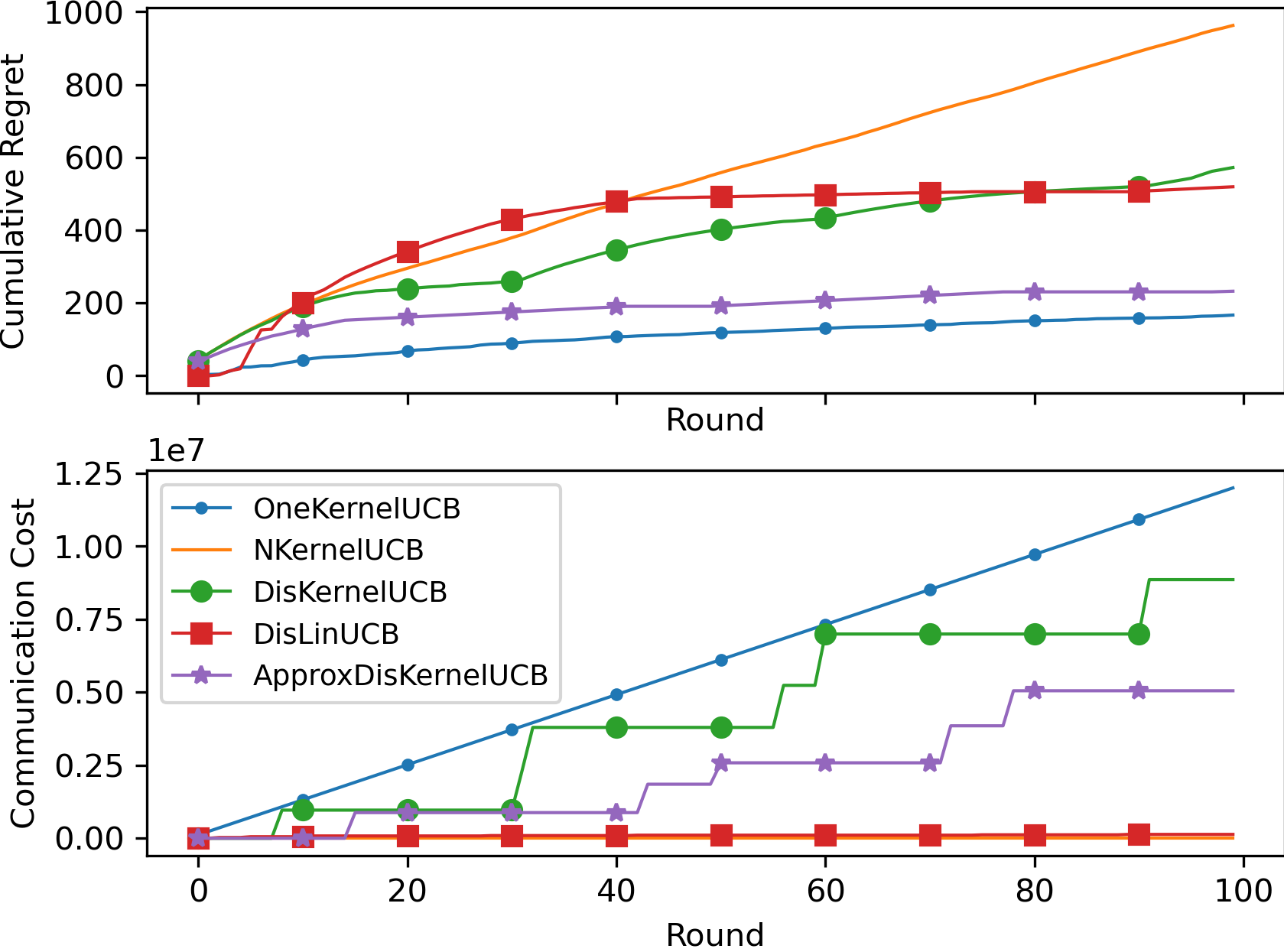
When examining the experiment results presented in Figure 1, 2 and 3, we can first look at the cumulative regret and communication cost of OneKernelUCB and NKernelUCB, which correspond to the two extreme cases where the clients communicate in every time step to learn a shared model, and each client learns its own model independently with no communication, respectively. OneKernelUCB achieves the smallest cumulative regret in all experiments, while also incurring the highest communication cost, i.e., O(TN2d)O(TN^{2}d). This demonstrates the need of efficient data aggregation across clients for reducing regret. Second, we can observe that DisKernelUCB incurs the second highest communication cost in all experiments due to the transfer of raw data, as we have discussed in Remark 2, which makes it prohibitively expensive for distributed setting. On the other extreme, we can see that DisLinUCB incurs very small communication cost thanks to its closed-form solution, but fails to capture the complicated reward mappings in most of these datasets, e.g. in Figure 1(a), 2(b) and 3(a), it leads to even worse regret than NKernelUCB that learns a kernelized bandit model independently for each client. In comparison, the proposed Approx-DisKernelUCB algorithm enjoys the best of both worlds in most cases, i.e., it can take advantage of the superior modeling power of kernels to reduce regret, while only requiring a relatively low communication cost for clients to collaborate. On all the datasets, Approx-DisKernelUCB achieved comparable regret with DisKernelUCB that maintains exact kernelized estimators, and sometimes even getting very close to OneKernelUCB, e.g., in Figure 1(b) and 2(a), but its communication cost is only slightly higher than that of DisLinUCB.

6 Conclusion

In this paper, we proposed the first communication efficient algorithm for distributed kernel bandits using Nyström approximation. Clients in the learning system project their local data to a finite RKHS spanned by a shared dictionary, and then communicate the embedded statistics for collaborative exploration. To ensure communication efficiency, the frequency of dictionary update and synchronization of embedded statistics are controlled by an event-trigger. The algorithm is proved to incur O(N2γNT3)O(N^{2}\gamma_{NT}^{3}) communication cost, while attaining the optimal O(NTγNT)O(\sqrt{NT}\gamma_{NT}) cumulative regret.

We should note that the total number of synchronizations required by Approx-DisKernelUCB is NγNTN\gamma_{NT}, which is N\sqrt{N} worse than DisKernelUCB. An important future direction of this work is to investigate whether this part can be further improved. It is also interesting to extend the proposed algorithm to P2P setting, at the absence of a central server to coordinate the update of the shared dictionary and the exchange of embedded statistics. Due to the delay in propagating messages, it may be beneficial to utilize possible local structures in the network of clients, and approximate each block of the kernel matrix separately (Si et al., 2014), i.e., each block corresponds to a group of clients, instead of directly approximating the complete matrix.

7 Acknowledgement

This work is supported by NSF grants IIS-2128019, IIS-1838615, IIS-1553568, IIS-2107304, CMMI-1653435, AFOSR grant and ONR grant 1006977.

References

  • Abbasi-Yadkori et al. (2011) Yasin Abbasi-Yadkori, Dávid Pál, and Csaba Szepesvári. Improved algorithms for linear stochastic bandits. Advances in neural information processing systems, 24:2312–2320, 2011.
  • Ban et al. (2021) Yikun Ban, Yuchen Yan, Arindam Banerjee, and Jingrui He. Ee-net: Exploitation-exploration neural networks in contextual bandits. arXiv preprint arXiv:2110.03177, 2021.
  • Calandriello et al. (2017) Daniele Calandriello, Alessandro Lazaric, and Michal Valko. Second-order kernel online convex optimization with adaptive sketching. In International Conference on Machine Learning, pages 645–653. PMLR, 2017.
  • Calandriello et al. (2019) Daniele Calandriello, Luigi Carratino, Alessandro Lazaric, Michal Valko, and Lorenzo Rosasco. Gaussian process optimization with adaptive sketching: Scalable and no regret. In Conference on Learning Theory, pages 533–557. PMLR, 2019.
  • Calandriello et al. (2020) Daniele Calandriello, Luigi Carratino, Alessandro Lazaric, Michal Valko, and Lorenzo Rosasco. Near-linear time gaussian process optimization with adaptive batching and resparsification. In International Conference on Machine Learning, pages 1295–1305. PMLR, 2020.
  • Chowdhury and Gopalan (2017) Sayak Ray Chowdhury and Aditya Gopalan. On kernelized multi-armed bandits. In International Conference on Machine Learning, pages 844–853. PMLR, 2017.
  • Du et al. (2021) Yihan Du, Wei Chen, Yuko Yuroki, and Longbo Huang. Collaborative pure exploration in kernel bandit. arXiv preprint arXiv:2110.15771, 2021.
  • Dua and Graff (2017) Dheeru Dua and Casey Graff. UCI machine learning repository, 2017. URL http://archive.ics.uci.edu/ml.
  • Dubey and Pentland (2020) Abhimanyu Dubey and AlexSandy’ Pentland. Differentially-private federated linear bandits. Advances in Neural Information Processing Systems, 33, 2020.
  • Dubey et al. (2020) Abhimanyu Dubey et al. Kernel methods for cooperative multi-agent contextual bandits. In International Conference on Machine Learning, pages 2740–2750. PMLR, 2020.
  • Durand et al. (2018) Audrey Durand, Charis Achilleos, Demetris Iacovides, Katerina Strati, Georgios D Mitsis, and Joelle Pineau. Contextual bandits for adapting treatment in a mouse model of de novo carcinogenesis. In Machine learning for healthcare conference, pages 67–82. PMLR, 2018.
  • Filippi et al. (2010) Sarah Filippi, Olivier Cappe, Aurélien Garivier, and Csaba Szepesvári. Parametric bandits: The generalized linear case. In NIPS, volume 23, pages 586–594, 2010.
  • Harper and Konstan (2015) F Maxwell Harper and Joseph A Konstan. The movielens datasets: History and context. Acm transactions on interactive intelligent systems (tiis), 5(4):1–19, 2015.
  • He et al. (2022) Jiafan He, Tianhao Wang, Yifei Min, and Quanquan Gu. A simple and provably efficient algorithm for asynchronous federated contextual linear bandits. arXiv preprint arXiv:2207.03106, 2022.
  • Hillel et al. (2013) Eshcar Hillel, Zohar S Karnin, Tomer Koren, Ronny Lempel, and Oren Somekh. Distributed exploration in multi-armed bandits. Advances in Neural Information Processing Systems, 26, 2013.
  • Huang et al. (2013) Junxian Huang, Feng Qian, Yihua Guo, Yuanyuan Zhou, Qiang Xu, Z Morley Mao, Subhabrata Sen, and Oliver Spatscheck. An in-depth study of lte: Effect of network protocol and application behavior on performance. ACM SIGCOMM Computer Communication Review, 43(4):363–374, 2013.
  • Huang et al. (2021) Ruiquan Huang, Weiqiang Wu, Jing Yang, and Cong Shen. Federated linear contextual bandits. Advances in Neural Information Processing Systems, 34, 2021.
  • Korda et al. (2016) Nathan Korda, Balazs Szorenyi, and Shuai Li. Distributed clustering of linear bandits in peer to peer networks. In International conference on machine learning, pages 1301–1309. PMLR, 2016.
  • Li and Wang (2022) Chuanhao Li and Hongning Wang. Asynchronous upper confidence bound algorithms for federated linear bandits. In International Conference on Artificial Intelligence and Statistics, pages 6529–6553. PMLR, 2022.
  • Li et al. (2010a) Lihong Li, Wei Chu, John Langford, and Robert E Schapire. A contextual-bandit approach to personalized news article recommendation. In Proceedings of the 19th international conference on World wide web, pages 661–670, 2010a.
  • Li et al. (2010b) Wei Li, Xuerui Wang, Ruofei Zhang, Ying Cui, Jianchang Mao, and Rong Jin. Exploitation and exploration in a performance based contextual advertising system. In Proceedings of the 16th ACM SIGKDD international conference on Knowledge discovery and data mining, pages 27–36, 2010b.
  • Nyström (1930) Evert J Nyström. Über die praktische auflösung von integralgleichungen mit anwendungen auf randwertaufgaben. Acta Mathematica, 54:185–204, 1930.
  • Scarlett et al. (2017) Jonathan Scarlett, Ilija Bogunovic, and Volkan Cevher. Lower bounds on regret for noisy gaussian process bandit optimization. In Conference on Learning Theory, pages 1723–1742. PMLR, 2017.
  • Shi and Shen (2021) Chengshuai Shi and Cong Shen. Federated multi-armed bandits. In Proceedings of the 35th AAAI Conference on Artificial Intelligence (AAAI), 2021.
  • Si et al. (2014) Si Si, Cho-Jui Hsieh, and Inderjit Dhillon. Memory efficient kernel approximation. In International Conference on Machine Learning, pages 701–709. PMLR, 2014.
  • Srinivas et al. (2009) Niranjan Srinivas, Andreas Krause, Sham M Kakade, and Matthias Seeger. Gaussian process optimization in the bandit setting: No regret and experimental design. arXiv preprint arXiv:0912.3995, 2009.
  • Tao et al. (2019) Chao Tao, Qin Zhang, and Yuan Zhou. Collaborative learning with limited interaction: Tight bounds for distributed exploration in multi-armed bandits. In 2019 IEEE 60th Annual Symposium on Foundations of Computer Science (FOCS), pages 126–146. IEEE, 2019.
  • Vakili et al. (2021) Sattar Vakili, Kia Khezeli, and Victor Picheny. On information gain and regret bounds in gaussian process bandits. In International Conference on Artificial Intelligence and Statistics, pages 82–90. PMLR, 2021.
  • Valko et al. (2013) Michal Valko, Nathaniel Korda, Rémi Munos, Ilias Flaounas, and Nelo Cristianini. Finite-time analysis of kernelised contextual bandits. arXiv preprint arXiv:1309.6869, 2013.
  • Wang et al. (2019) Yuanhao Wang, Jiachen Hu, Xiaoyu Chen, and Liwei Wang. Distributed bandit learning: Near-optimal regret with efficient communication. In International Conference on Learning Representations, 2019.
  • Zenati et al. (2022) Houssam Zenati, Alberto Bietti, Eustache Diemert, Julien Mairal, Matthieu Martin, and Pierre Gaillard. Efficient kernel ucb for contextual bandits. arXiv preprint arXiv:2202.05638, 2022.
  • Zhou et al. (2020) Dongruo Zhou, Lihong Li, and Quanquan Gu. Neural contextual bandits with ucb-based exploration. In International Conference on Machine Learning, pages 11492–11502. PMLR, 2020.

A Technical Lemmas

Lemma 7 (Lemma 12 of (Abbasi-Yadkori et al., 2011))

Let AA, BB and CC be positive semi-definite matrices with finite dimension, such that A=B+CA=B+C. Then, we have that:

sup𝐱0𝐱A𝐱𝐱B𝐱det(A)det(B)\displaystyle\sup_{\mathbf{x}\neq\textbf{0}}\frac{\mathbf{x}^{\top}A\mathbf{x}}{\mathbf{x}^{\top}B\mathbf{x}}\leq\frac{\det(A)}{\det(B)}
Lemma 8 (Extension of Lemma 7 to kernel matrix)

Define positive definite matrices A=λ𝐈+𝚽1𝚽1+𝚽2𝚽2A=\lambda\mathbf{I}+\mathbf{\Phi}_{1}^{\top}\mathbf{\Phi}_{1}+\mathbf{\Phi}_{2}^{\top}\mathbf{\Phi}_{2} and B=λ𝐈+𝚽1𝚽1B=\lambda\mathbf{I}+\mathbf{\Phi}_{1}^{\top}\mathbf{\Phi}_{1}, where 𝚽1𝚽1,𝚽2𝚽2p×p\mathbf{\Phi}_{1}^{\top}\mathbf{\Phi}_{1},\mathbf{\Phi}_{2}^{\top}\mathbf{\Phi}_{2}\in\mathbb{R}^{p\times p} and pp is possibly infinite. Then, we have that:

supϕ0ϕAϕϕBϕdet(𝐈+λ1𝐊A)det(𝐈+λ1𝐊B)\displaystyle\sup_{\phi\neq\textbf{0}}\frac{\phi^{\top}A\phi}{\phi^{\top}B\phi}\leq\frac{\det(\mathbf{I}+\lambda^{-1}\mathbf{K}_{A})}{\det(\mathbf{I}+\lambda^{-1}\mathbf{K}_{B})}

where 𝐊A=[𝚽1𝚽2][𝚽1,𝚽2]\mathbf{K}_{A}=\begin{bmatrix}\mathbf{\Phi}_{1}\\ \mathbf{\Phi}_{2}\end{bmatrix}\begin{bmatrix}\mathbf{\Phi}_{1}^{\top},\mathbf{\Phi}_{2}^{\top}\end{bmatrix} and 𝐊B=𝚽1𝚽1\mathbf{K}_{B}=\mathbf{\Phi}_{1}\mathbf{\Phi}_{1}^{\top}.

Proof [Proof of Lemma 8] Similar to the proof of Lemma 12 of (Abbasi-Yadkori et al., 2011), we start from the simple case when 𝚽2𝚽2=mm\mathbf{\Phi}_{2}^{\top}\mathbf{\Phi}_{2}=mm^{\top}, where mpm\in\mathbb{R}^{p}. Using Cauchy-Schwartz inequality, we have

(ϕm)2=(ϕB1/2B1/2m)2B1/2ϕ2B1/2m2=ϕB2mB12,\displaystyle(\phi^{\top}m)^{2}=(\phi^{\top}B^{1/2}B^{-1/2}m)^{2}\leq\lVert B^{1/2}\phi\rVert^{2}\lVert B^{-1/2}m\rVert^{2}=\lVert\phi\rVert^{2}_{B}\lVert m\rVert^{2}_{B^{-1}},

and thus,

ϕ(B+mm)ϕϕBϕ+ϕB2mB12=(1+mB12)ϕB2,\displaystyle\phi^{\top}(B+mm^{\top})\phi\leq\phi^{\top}B\phi+\lVert\phi\rVert^{2}_{B}\lVert m\rVert^{2}_{B^{-1}}=(1+\lVert m\rVert^{2}_{B^{-1}})\lVert\phi\rVert^{2}_{B},

so we have

ϕAϕϕBϕ1+mB12\displaystyle\frac{\phi^{\top}A\phi}{\phi^{\top}B\phi}\leq 1+\lVert m\rVert_{B^{-1}}^{2}

for any ϕ\phi. Then using the kernel trick, e.g., see the derivation of Eq (27) in Zenati et al. (2022), we have

1+mB12=det(𝐈+λ1𝐊A)det(𝐈+λ1𝐊B),\displaystyle 1+\lVert m\rVert_{B^{-1}}^{2}=\frac{\det(\mathbf{I}+\lambda^{-1}\mathbf{K}_{A})}{\det(\mathbf{I}+\lambda^{-1}\mathbf{K}_{B})},

which finishes the proof of this simple case. Now consider the general case where 𝚽2𝚽2=m1m1+m2m2++mt1mt1\mathbf{\Phi}_{2}^{\top}\mathbf{\Phi}_{2}=m_{1}m_{1}^{\top}+m_{2}m_{2}^{\top}+\dots+m_{t-1}m_{t-1}^{\top}. Let’s define Vs=B+m1m1+m2m2++ms1ms1V_{s}=B+m_{1}m_{1}^{\top}+m_{2}m_{2}^{\top}+\dots+m_{s-1}m_{s-1}^{\top} and the corresponding kernel matrix 𝐊Vs=[𝚽1m1ms1][𝚽1,m1,,ms1]\mathbf{K}_{V_{s}}=\begin{bmatrix}\mathbf{\Phi}_{1}\\ m_{1}^{\top}\\ \dots\\ m_{s-1}^{\top}\end{bmatrix}\begin{bmatrix}\mathbf{\Phi}_{1}^{\top},m_{1},\dots,m_{s-1}\end{bmatrix}, and note that ϕAϕϕBϕ=ϕVtϕϕVt1ϕϕVt1ϕϕVt2ϕϕV2ϕϕBϕ\frac{\phi^{\top}A\phi}{\phi^{\top}B\phi}=\frac{\phi^{\top}V_{t}\phi}{\phi^{\top}V_{t-1}\phi}\frac{\phi^{\top}V_{t-1}\phi}{\phi^{\top}V_{t-2}\phi}\dots\frac{\phi^{\top}V_{2}\phi}{\phi^{\top}B\phi}. Then we can apply the result for the simple case on each term in the product above, which gives us

ϕAϕϕBϕ\displaystyle\frac{\phi^{\top}A\phi}{\phi^{\top}B\phi} det(𝐈+λ1𝐊Vt)det(𝐈+λ1𝐊Vt1)det(𝐈+λ1𝐊Vt1)det(𝐈+λ1𝐊Vt2)det(𝐈+λ1𝐊V2)det(𝐈+λ1𝐊B)\displaystyle\leq\frac{\det(\mathbf{I}+\lambda^{-1}\mathbf{K}_{V_{t}})}{\det(\mathbf{I}+\lambda^{-1}\mathbf{K}_{V_{t-1}})}\frac{\det(\mathbf{I}+\lambda^{-1}\mathbf{K}_{V_{t-1}})}{\det(\mathbf{I}+\lambda^{-1}\mathbf{K}_{V_{t-2}})}\dots\frac{\det(\mathbf{I}+\lambda^{-1}\mathbf{K}_{V_{2}})}{\det(\mathbf{I}+\lambda^{-1}\mathbf{K}_{B})}
=det(𝐈+λ1𝐊Vt)det(𝐈+λ1𝐊B)=det(𝐈+λ1𝐊A)det(𝐈+λ1𝐊B),\displaystyle=\frac{\det(\mathbf{I}+\lambda^{-1}\mathbf{K}_{V_{t}})}{\det(\mathbf{I}+\lambda^{-1}\mathbf{K}_{B})}=\frac{\det(\mathbf{I}+\lambda^{-1}\mathbf{K}_{A})}{\det(\mathbf{I}+\lambda^{-1}\mathbf{K}_{B})},

which finishes the proof.


Lemma 9 (Eq (26) and Eq (27) of Zenati et al. (2022))

Let {ϕt}t=1\{\phi_{t}\}_{t=1}^{\infty} be a sequence in p\mathbb{R}^{p}, Vp×pV\in\mathbb{R}^{p\times p} a positive definite matrix, where pp is possibly infinite, and define Vt=V+s=1tϕsϕsV_{t}=V+\sum_{s=1}^{t}\phi_{s}\phi_{s}^{\top}. Then we have that

t=1nmin(ϕtVt112,1)2ln(det(𝐈+λ1𝐊Vt)),\displaystyle\sum_{t=1}^{n}\min\bigl{(}\lVert\phi_{t}\rVert^{2}_{V_{t-1}^{-1}},1\bigr{)}\leq 2\ln\bigl{(}\det(\mathbf{I}+\lambda^{-1}\mathbf{K}_{V_{t}})\bigr{)},

where 𝐊Vt\mathbf{K}_{V_{t}} is the kernel matrix corresponding to VtV_{t} as defined in Lemma 8.

Lemma 10 (Lemma 4 of (Calandriello et al., 2020))

For t>tlastt>t_{\text{last}}, we have for any 𝐱d\mathbf{x}\in\mathbb{R}^{d}

σ^t2(𝐱)σ^tlast2(𝐱)(1+s=tlast+1tσ^tlast2(𝐱s))σ^t2(𝐱)\displaystyle\hat{\sigma}_{t}^{2}(\mathbf{x})\leq\hat{\sigma}_{t_{\text{last}}}^{2}(\mathbf{x})\leq\bigl{(}1+\sum_{s=t_{\text{last}}+1}^{t}\hat{\sigma}_{t_{\text{last}}}^{2}(\mathbf{x}_{s})\bigr{)}\hat{\sigma}_{t}^{2}(\mathbf{x})

B Confidence Ellipsoid for DisKernelUCB

In this section, we construct the confidence ellipsoid for DisKernelUCB as shown in Lemma 11.

Lemma 11 (Confidence Ellipsoid for DisKernelUCB)

Let δ(0,1)\delta\in(0,1). With probability at least 1δ1-\delta, for all t[NT],i[N]t\in[NT],i\in[N], we have

θ^t,iθ𝐀t,iλθ+R2ln(N/δ)+ln(det(𝐊𝒟t(i),𝒟t(i)/λ+𝐈)).\displaystyle\lVert\hat{\theta}_{t,i}-\theta_{\star}\rVert_{\mathbf{A}_{t,i}}\leq\sqrt{\lambda}\lVert\theta_{\star}\rVert+R\sqrt{2\ln(N/\delta)+\ln(\det(\mathbf{K}_{\mathcal{D}_{t}(i),\mathcal{D}_{t}(i)}/\lambda+\mathbf{I}))}.

The analysis is rooted in (Zenati et al., 2022) for kernelized contextual bandit, but with non-trivial extensions: we adopted the stopping time argument from (Abbasi-Yadkori et al., 2011) to remove a logarithmic factor in TT (this improvement is hinted in Section 3.3 of (Zenati et al., 2022) as well); and this stopping time argument is based on a special ‘batched filtration’ that is different for each client, which is required to address the dependencies due to the event-triggered distributed communication. This problem also exists in prior works of distributed linear bandit, but was not addressed rigorously (see Lemma H.1. of (Wang et al., 2019)).

Recall that the Ridge regression estimator

θ^t,i\displaystyle\hat{\theta}_{t,i} =𝐀t,i1s𝒟t(i)ϕsys=𝐀t,i1s𝒟t(i)ϕs(ϕsθ+ηs)\displaystyle=\mathbf{A}_{t,i}^{-1}\sum_{s\in\mathcal{D}_{t}(i)}\phi_{s}y_{s}=\mathbf{A}_{t,i}^{-1}\sum_{s\in\mathcal{D}_{t}(i)}\phi_{s}(\phi_{s}^{\top}\theta_{\star}+\eta_{s})
=θλ𝐀t,i1θ+𝐀t,i1s𝒟t(i)ϕsηs,\displaystyle=\theta_{\star}-\lambda\mathbf{A}_{t,i}^{-1}\theta_{\star}+\mathbf{A}_{t,i}^{-1}\sum_{s\in\mathcal{D}_{t}(i)}\phi_{s}\eta_{s},

and thus, we have

𝐀t,i1/2(θ^t,iθ)=λ𝐀t,i1/2θ+𝐀t,i1/2s𝒟t(i)ϕsηsλ𝐀t,i1/2θ+𝐀t,i1/2s𝒟t(i)ϕsηsλθ+𝐀t,i1/2s𝒟t(i)ϕsηs\begin{split}\lVert\mathbf{A}_{t,i}^{1/2}(\hat{\theta}_{t,i}-\theta_{\star})\rVert&=\lVert-\lambda\mathbf{A}_{t,i}^{-1/2}\theta_{\star}+\mathbf{A}_{t,i}^{-1/2}\sum_{s\in\mathcal{D}_{t}(i)}\phi_{s}\eta_{s}\rVert\\ &\leq\lVert\lambda\mathbf{A}_{t,i}^{-1/2}\theta_{\star}\rVert+\lVert\mathbf{A}_{t,i}^{-1/2}\sum_{s\in\mathcal{D}_{t}(i)}\phi_{s}\eta_{s}\rVert\\ &\leq\sqrt{\lambda}\lVert\theta_{\star}\rVert+\lVert\mathbf{A}_{t,i}^{-1/2}\sum_{s\in\mathcal{D}_{t}(i)}\phi_{s}\eta_{s}\rVert\end{split} (5)

where the first inequality is due to the triangle inequality, and the second is due to the property of Rayleigh quotient, i.e., 𝐀t,i1/2θθλmax(𝐀t,i1)θ1λ\lVert\mathbf{A}_{t,i}^{-1/2}\theta_{\star}\rVert\leq\lVert\theta_{\star}\rVert\sqrt{\lambda_{max}(\mathbf{A}_{t,i}^{-1})}\leq\lVert\theta_{\star}\rVert\frac{1}{\sqrt{\lambda}}.

Difference from standard argument

Note that the second term may seem similar to the ones appear in the self-normalized bound in previous works of linear and kernelized bandits (Abbasi-Yadkori et al., 2011; Chowdhury and Gopalan, 2017; Zenati et al., 2022). However, a main difference is that 𝒟t(i)\mathcal{D}_{t}(i), i.e., the sequence of indices for the data points used to update client ii, is constructed using the event-trigger as defined in Eq (2) . The event-trigger is data-dependent, and thus it is a delayed and permuted version of the original sequence [t][t]. It is delayed in the sense that the length |𝒟t(i)|<t|\mathcal{D}_{t}(i)|<t unless tt is the global synchronization step. It is permuted in the sense that every client receives the data in a different order, i.e., before the synchronization, each client first updates using its local new data, and then receives data from other clients at the synchronization. This prevents us from directly applying Lemma 3.1 of (Zenati et al., 2022), and requires a careful construction of the filtration, as shown in the following paragraph.

Construction of filtration

For some client ii at time step tt, the sequence of time indices in 𝒟t(i)\mathcal{D}_{t}(i) is arranged in the order that client ii receives the corresponding data points, which includes both data added during local update in each client, and data received from the server during global synchronization. The former adds one data point at a time, while the latter adds a batch of data points, which, as we will see, break the assumption commonly made in standard self-normalized bound (Abbasi-Yadkori et al., 2011; Chowdhury and Gopalan, 2017; Zenati et al., 2022). Specifically, we denote 𝒟t(i)[k]\mathcal{D}_{t}(i)[k], for k|𝒟t(i)|k\leq|\mathcal{D}_{t}(i)|, as the kk-th element in this sequence, i.e., (𝐱𝒟t(i)[k],y𝒟t(i)[k])(\mathbf{x}_{\mathcal{D}_{t}(i)[k]},y_{\mathcal{D}_{t}(i)[k]}) is the kk-th data point received by client ii. Then we denote t(i)={k1,k2,}\mathcal{B}_{t}(i)=\{k_{1},k_{2},\dots\} as the sequence of kk’s that marks the end of each batch (a singel data point added by local update is also considered a batch). We can see that if the kk-th element is in the middle of a batch, i.e., k[kq1,kq]k\in[k_{q-1},k_{q}], it has dependency all the way to the kqk_{q}’s element, since this index can only be determined until some client triggers a global synchronization at time step 𝒟t(i)[kq]\mathcal{D}_{t}(i)[k_{q}].

Denote by k,i=σ((𝐱s,ηs)s𝒟(i)[1:k1],𝐱𝒟(i)[k])\mathcal{F}_{k,i}=\sigma\bigl{(}(\mathbf{x}_{s},\eta_{s})_{s\in\mathcal{D}_{\infty}(i)[1:k-1]},\mathbf{x}_{\mathcal{D}_{\infty}(i)[k]}\bigr{)} the σ\sigma-algebra generated by the sequence of data points up to the kk-th element in 𝒟(i)\mathcal{D}_{\infty}(i). As we mentioned, because of the dependency of the index on the future data points, for some kk-th element that is inside a batch, i.e., k[kq1,kq]k\in[k_{q-1},k_{q}], 𝐱𝒟(i)[k]\mathbf{x}_{\mathcal{D}_{\infty}(i)[k]} is not k,i\mathcal{F}_{k,i}-measurable and η𝒟(i)[k]\eta_{\mathcal{D}_{\infty}(i)[k]} is not k+1,i\mathcal{F}_{k+1,i}-measurable, which violate the assumption made in standard self-normalized bound (Abbasi-Yadkori et al., 2011; Chowdhury and Gopalan, 2017; Zenati et al., 2022). However, they become measurable if we condition on kq,i\mathcal{F}_{k_{q},i}. In addition, recall that in Section 3.1 we assume η𝒟(i)[k]\eta_{\mathcal{D}_{\infty}(i)[k]} is zero-mean RR-sub-Gaussian conditioned on σ((𝐱s,ηs)s𝒩𝒟(i)[k]1(i𝒟(i)[k]),𝐱𝒟(i)[k])\sigma\bigl{(}(\mathbf{x}_{s},\eta_{s})_{s\in\mathcal{N}_{\mathcal{D}_{\infty}(i)[k]-1}(i_{\mathcal{D}_{\infty}(i)[k]})},\mathbf{x}_{\mathcal{D}_{\infty}(i)[k]}\bigr{)}, which is the σ\sigma-algebra generated by the sequence of local data collected by client i𝒟(i)[k]i_{\mathcal{D}_{\infty}(i)[k]}. We can see that as σ((𝐱s,ηs)s𝒩𝒟(i)[k]1(i𝒟(i)[k]),𝐱𝒟(i)[k])k,i\sigma\bigl{(}(\mathbf{x}_{s},\eta_{s})_{s\in\mathcal{N}_{\mathcal{D}_{\infty}(i)[k]-1}(i_{\mathcal{D}_{\infty}(i)[k]})},\mathbf{x}_{\mathcal{D}_{\infty}(i)[k]}\bigr{)}\subseteq\mathcal{F}_{k,i}, η𝒟(i)[k]\eta_{\mathcal{D}_{\infty}(i)[k]} is zero-mean RR-sub-Gaussian conditioned on k,i\mathcal{F}_{k,i}. Basically, our assumption of RR-sub-Gaussianity conditioned on local sequence instead of global sequence of data points, prevents the situation where the noise depends on data points that have not been communicated to the current client yet, i.e., they are not included in k,i\mathcal{F}_{k,i}.

With our ‘batched filtration’ {k,i}k(i)\{\mathcal{F}_{k,i}\}_{k\in\mathcal{B}_{\infty}(i)} for each client ii, we have everything we need to establish a time-uniform self-normalized bound that resembles Lemma 3.1 of (Zenati et al., 2022), but with improved logarithmic factor using the stopping time argument from (Abbasi-Yadkori et al., 2011). Then we can take a union bound over NN clients to obtain the uniform bound over all clients and time steps.

Super-martingale & self-normalized bound

First, we need the following lemmas adopted from (Zenati et al., 2022) to our ‘batched filtration’.

Lemma 12

Let υd\upsilon\in\mathbb{R}^{d} be arbitrary and consider for any k(i)k\in\mathcal{B}_{\infty}(i), i[N]i\in[N], we have

Mk,iυ=exp(12λυυ+s𝒟(i)[1:k][ηs<υ,Xs>R12υXsXsυ])\displaystyle M_{k,i}^{\upsilon}=\exp\left(-\frac{1}{2}\lambda\upsilon^{\top}\upsilon+\sum_{s\in\mathcal{D}_{\infty}(i)[1:k]}[\frac{\eta_{s}<\upsilon,X_{s}>}{R}-\frac{1}{2}\upsilon^{\top}X_{s}X_{s}^{\top}\upsilon]\right)

is a k+1,i\mathcal{F}_{k+1,i}-super-martingale, and 𝔼[Mk,iυ]exp(12λυυ)\mathbb{E}[M_{k,i}^{\upsilon}]\leq\exp(-\frac{1}{2}\lambda\upsilon^{\top}\upsilon). Let k~\tilde{k} be a stopping time w.r.t. the filtration {k,i}k(i)\{\mathcal{F}_{k,i}\}_{k\in\mathcal{B}_{\infty}(i)}. Then Mk~,iυM_{\tilde{k},i}^{\upsilon} is almost surely well-defined and 𝔼[Mk~,iυ]1\mathbb{E}[M_{\tilde{k},i}^{\upsilon}]\leq 1.

Proof [Proof of Lemma 12] To show that {Mk,iυ}k(i)\{M_{k,i}^{\upsilon}\}_{k\in\mathcal{B}_{\infty}(i)} is a super-martinagle, we denote

Dk,iυ=exp(η𝒟(i)[k]<υ,X𝒟(i)[k]>R12<υ,X𝒟(i)[k]>2),\displaystyle D_{k,i}^{\upsilon}=\exp\left(\frac{\eta_{\mathcal{D}_{\infty}(i)[k]}<\upsilon,X_{\mathcal{D}_{\infty}(i)[k]}>}{R}-\frac{1}{2}<\upsilon,X_{\mathcal{D}_{\infty}(i)[k]}>^{2}\right),

with D0,iυ=exp(12λυυ)D_{0,i}^{\upsilon}=\exp(-\frac{1}{2}\lambda\upsilon^{\top}\upsilon), and as we have showed earlier, η𝒟(i)[k]\eta_{\mathcal{D}_{\infty}(i)[k]} is RR-sub-Gaussian conditioned on k,i\mathcal{F}_{k,i}. Therefore, 𝔼[Dk,iυ|k,i]1\mathbb{E}[D_{k,i}^{\upsilon}|\mathcal{F}_{k,i}]\leq 1. Moreover, Dk,iυD_{k,i}^{\upsilon} and Mk,iυM_{k,i}^{\upsilon} are k+1,i\mathcal{F}_{k+1,i}-measurable. Then we have

𝔼[Mk,iυ|k,i]\displaystyle\mathbb{E}[M_{k,i}^{\upsilon}|\mathcal{F}_{k,i}] =𝔼[D1,iυD2,iυDk1,iυDk,iυ|k,i]\displaystyle=\mathbb{E}[D_{1,i}^{\upsilon}D_{2,i}^{\upsilon}\dots D_{k-1,i}^{\upsilon}D_{k,i}^{\upsilon}|\mathcal{F}_{k,i}]
=D0,iυD1,iυD2,iυDk1,iυ𝔼[Dk,iυ|k,i]Mk1,iυ,\displaystyle=D_{0,i}^{\upsilon}D_{1,i}^{\upsilon}D_{2,i}^{\upsilon}\dots D_{k-1,i}^{\upsilon}\mathbb{E}[D_{k,i}^{\upsilon}|\mathcal{F}_{k,i}]\leq M_{k-1,i}^{\upsilon},

which shows {Mk,iυ}k(i)\{M_{k,i}^{\upsilon}\}_{k\in\mathcal{B}_{\infty}(i)} is a super-martinagle, with 𝔼[Mk,iυ]D0,iυ=exp(12λυυ)\mathbb{E}[M_{k,i}^{\upsilon}]\leq D_{0,i}^{\upsilon}=\exp(-\frac{1}{2}\lambda\upsilon^{\top}\upsilon). Then using the same argument as Lemma 8 of (Abbasi-Yadkori et al., 2011), we have that Mk~,iυM_{\tilde{k},i}^{\upsilon} is almost surely well-defined, and 𝔼[Mk~,iυ]D0,iυ=exp(12λυυ)\mathbb{E}[M_{\tilde{k},i}^{\upsilon}]\leq D_{0,i}^{\upsilon}=\exp(-\frac{1}{2}\lambda\upsilon^{\top}\upsilon).  

Lemma 13

Let k~\tilde{k} be a stopping time w.r.t. the filtration {k,i}k(i)\{\mathcal{F}_{k,i}\}_{k\in\mathcal{B}_{\infty}(i)}. Then for δ>0\delta>0, we have

P((λ𝐈+s𝒟(i)[1:k~]XsXs)1/2(s𝒟(i)[1:k~]Xsηs)>R2ln(1/δ)+ln(det(𝐊𝒟(i)[1:k~],𝒟(i)[1:k~]/λ+𝐈)))\displaystyle P\Big{(}\lVert(\lambda\mathbf{I}+\sum_{s\in\mathcal{D}_{\infty}(i)[1:\tilde{k}]}X_{s}X_{s}^{\top})^{-1/2}(\sum_{s\in\mathcal{D}_{\infty}(i)[1:\tilde{k}]}X_{s}\eta_{s})\rVert>R\sqrt{2\ln(1/\delta)+\ln(\det(\mathbf{K}_{\mathcal{D}_{\infty}(i)[1:\tilde{k}],\mathcal{D}_{\infty}(i)[1:\tilde{k}]}/\lambda+\mathbf{I}))}\Big{)}
δ.\displaystyle\leq\delta.

Proof [Proof of Lemma 13] Using m:=(λ𝐈+s𝒟(i)[1:k]XsXs)1(s𝒟(i)[1:k]Xsηs)m:=(\lambda\mathbf{I}+\sum_{s\in\mathcal{D}_{\infty}(i)[1:k]}X_{s}X_{s}^{\top})^{-1}(\sum_{s\in\mathcal{D}_{\infty}(i)[1:k]}X_{s}\eta_{s}), we can rewrite Mk~,iυM_{\tilde{k},i}^{\upsilon} as

Mk~,iυ\displaystyle M_{\tilde{k},i}^{\upsilon} =exp(12(υm)(λ𝐈+s𝒟(i)[1:k]XsXs)(υm))\displaystyle=\exp\left(-\frac{1}{2}(\upsilon-m)^{\top}(\lambda\mathbf{I}+\sum_{s\in\mathcal{D}_{\infty}(i)[1:k]}X_{s}X_{s}^{\top})(\upsilon-m)\right)
×exp(12(λ𝐈+s𝒟(i)[1:k]XsXs)1/2(s𝒟(i)[1:k]Xsηs)2).\displaystyle\quad\times\exp\left(\frac{1}{2}\lVert(\lambda\mathbf{I}+\sum_{s\in\mathcal{D}_{\infty}(i)[1:k]}X_{s}X_{s}^{\top})^{-1/2}(\sum_{s\in\mathcal{D}_{\infty}(i)[1:k]}X_{s}\eta_{s})\rVert^{2}\right).

Then based on Lemma 12, we have

𝔼[exp(12(υm)(λ𝐈+s𝒟(i)[1:k]XsXs)(υm))]\displaystyle\mathbb{E}\Big{[}\exp\Big{(}-\frac{1}{2}(\upsilon-m)^{\top}(\lambda\mathbf{I}+\sum_{s\in\mathcal{D}_{\infty}(i)[1:k]}X_{s}X_{s}^{\top})(\upsilon-m)\Big{)}\Big{]}
+𝔼[exp(12(λ𝐈+s𝒟(i)[1:k]XsXs)1/2(s𝒟(i)[1:k]Xsηs)2)]exp(12λυυ)\displaystyle\quad+\mathbb{E}\Big{[}\exp\Big{(}\frac{1}{2}\lVert(\lambda\mathbf{I}+\sum_{s\in\mathcal{D}_{\infty}(i)[1:k]}X_{s}X_{s}^{\top})^{-1/2}(\sum_{s\in\mathcal{D}_{\infty}(i)[1:k]}X_{s}\eta_{s})\rVert^{2}\Big{)}\Big{]}\leq\exp(-\frac{1}{2}\lambda\upsilon^{\top}\upsilon)

Following the Laplace’s method as in proof of Lemma 3.1 of (Zenati et al., 2022), we have

𝔼[exp(12(λ𝐈+s𝒟(i)[1:k~]XsXs)1/2(s𝒟(i)[1:k~]Xsηs)2)]det(𝐊𝒟(i)[1:k~],𝒟(i)[1:k~]+λ𝐈)λk~\displaystyle\mathbb{E}\Big{[}\exp\Big{(}\frac{1}{2}\lVert(\lambda\mathbf{I}+\sum_{s\in\mathcal{D}_{\infty}(i)[1:\tilde{k}]}X_{s}X_{s}^{\top})^{-1/2}(\sum_{s\in\mathcal{D}_{\infty}(i)[1:\tilde{k}]}X_{s}\eta_{s})\rVert^{2}\Big{)}\Big{]}\leq\sqrt{\frac{\det(\mathbf{K}_{\mathcal{D}_{\infty}(i)[1:\tilde{k}],\mathcal{D}_{\infty}(i)[1:\tilde{k}]}+\lambda\mathbf{I})}{\lambda^{\tilde{k}}}}

By applying Markov-Chernov bound, we finish the proof.  

Proof of Lemma 11

Now using the stopping time argument as in (Abbasi-Yadkori et al., 2011), and a union bound over clients, we can bound the second term in Eq (5). First, define the bad event

Bk(δ)={ωΩ:(λ𝐈+\displaystyle B_{k}(\delta)=\bigl{\{}\omega\in\Omega:\lVert(\lambda\mathbf{I}+ s𝒟(i)[1:k]XsXs)1/2(s𝒟(i)[1:k]Xsηs)>\displaystyle\sum_{s\in\mathcal{D}_{\infty}(i)[1:k]}X_{s}X_{s}^{\top})^{-1/2}(\sum_{s\in\mathcal{D}_{\infty}(i)[1:k]}X_{s}\eta_{s})\rVert>
R2ln(1/δ)+ln(det(𝐊𝒟(i)[1:k],𝒟(i)[1:k]/λ+𝐈))},\displaystyle R\sqrt{2\ln(1/\delta)+\ln(\det(\mathbf{K}_{\mathcal{D}_{\infty}(i)[1:k],\mathcal{D}_{\infty}(i)[1:k]}/\lambda+\mathbf{I}))}\bigr{\}},

and k~(ω)=min(k0:ωBk(δ))\tilde{k}(\omega)=\min(k\geq 0:\omega\in B_{k}(\delta)), which is a stopping time. Moreover, k(i)Bk(δ)={ω:k~<}\cup_{k\in\mathcal{B}_{\infty}(i)}B_{k}(\delta)=\{\omega:\tilde{k}<\infty\}. Then using Lemma 13, we have

P(k(i)Bk(δ))=P(k~<)\displaystyle P\bigl{(}\cup_{k\in\mathcal{B}_{\infty}(i)}B_{k}(\delta)\bigr{)}=P(\tilde{k}<\infty)
P((λ𝐈+s𝒟(i)[1:k~]XsXs)1/2(s𝒟(i)[1:k~]Xsηs)>R2ln(1/δ)+ln(det(𝐊𝒟(i)[1:k~],𝒟(i)[1:k~]/λ+𝐈)))\displaystyle\leq P\Big{(}\lVert(\lambda\mathbf{I}+\sum_{s\in\mathcal{D}_{\infty}(i)[1:\tilde{k}]}X_{s}X_{s}^{\top})^{-1/2}(\sum_{s\in\mathcal{D}_{\infty}(i)[1:\tilde{k}]}X_{s}\eta_{s})\rVert>R\sqrt{2\ln(1/\delta)+\ln(\det(\mathbf{K}_{\mathcal{D}_{\infty}(i)[1:\tilde{k}],\mathcal{D}_{\infty}(i)[1:\tilde{k}]}/\lambda+\mathbf{I}))}\Big{)}
δ\displaystyle\leq\delta

Note that (i)\mathcal{B}_{\infty}(i) is the sequence of indices kk in 𝒟(i)\mathcal{D}_{\infty}(i) when client ii gets updated. Therefore, the result above is equivalent to

𝐀t,i1/2s𝒟t(i)ϕsηsR2ln(1/δ)+ln(det(𝐊𝒟t(i),𝒟t(i)/λ+𝐈))\displaystyle\lVert\mathbf{A}_{t,i}^{-1/2}\sum_{s\in\mathcal{D}_{t}(i)}\phi_{s}\eta_{s}\rVert\leq R\sqrt{2\ln(1/\delta)+\ln(\det(\mathbf{K}_{\mathcal{D}_{t}(i),\mathcal{D}_{t}(i)}/\lambda+\mathbf{I}))}

for all t1t\geq 1, with probability at least 1δ1-\delta. Then by taking a union bound over NN clients, we finish the proof.

C Proof of Lemma 1: Regret and Communication Cost of DisKernelUCB

Based on Lemma 11 and the arm selection rule in Eq (1), we have

f(𝐱t)\displaystyle f(\mathbf{x}_{t}^{\star}) μ^t1,it(𝐱t)+αt1,itσ^t1,it(𝐱t)μ^t1,it(𝐱t)+αt1,itσ^t1,it(𝐱t),\displaystyle\leq\hat{\mu}_{t-1,i_{t}}(\mathbf{x}_{t}^{\star})+\alpha_{t-1,i_{t}}\hat{\sigma}_{t-1,i_{t}}(\mathbf{x}_{t}^{\star})\leq\hat{\mu}_{t-1,i_{t}}(\mathbf{x}_{t})+\alpha_{t-1,i_{t}}\hat{\sigma}_{t-1,i_{t}}(\mathbf{x}_{t}),
f(𝐱t)\displaystyle f(\mathbf{x}_{t}) μ^t1,it(𝐱t)αt1,itσ^t1,it(𝐱t),\displaystyle\geq\hat{\mu}_{t-1,i_{t}}(\mathbf{x}_{t})-\alpha_{t-1,i_{t}}\hat{\sigma}_{t-1,i_{t}}(\mathbf{x}_{t}),

and thus rt=f(𝐱t)f(𝐱t)2αt1,itσ^t1,it(𝐱t)r_{t}=f(\mathbf{x}_{t}^{\star})-f(\mathbf{x}_{t})\leq 2\alpha_{t-1,i_{t}}\hat{\sigma}_{t-1,i_{t}}(\mathbf{x}_{t}), for all t[NT]t\in[NT], with probability at least 1δ1-\delta. Then following similar steps as DisLinUCB of (Wang et al., 2019), we can obtain the regret and communication cost upper bound of DisKernelUCB.

C.1 Regret Upper Bound

We call the time period in-between two consecutive global synchronizations as an epoch, i.e., the pp-th epoch refers to [tp1+1,tp][t_{p-1}+1,t_{p}], where p[B]p\in[B] and 0BNT0\leq B\leq NT denotes the total number of global synchronizations. Now consider an imaginary centralized agent that has immediate access to each data point in the learning system, and denote by At=s=1tϕsϕsA_{t}=\sum_{s=1}^{t}\phi_{s}\phi_{s}^{\top} and 𝐊[t],[t]\mathbf{K}_{[t],[t]} for t[NT]t\in[NT] the covariance matrix and kernel matrix constructed by this centralized agent. Then similar to (Wang et al., 2019), we call the pp-th epoch a good epoch if

ln(det(𝐈+λ1𝐊[tp],[tp])det(𝐈+λ1𝐊[tp1],[tp1]))1,\displaystyle\ln\left(\frac{\det(\mathbf{I}+\lambda^{-1}\mathbf{K}_{[t_{p}],[t_{p}]})}{\det(\mathbf{I}+\lambda^{-1}\mathbf{K}_{[t_{p-1}],[t_{p-1}]})}\right)\leq 1,

otherwise it is a bad epoch. Note that ln(det(I+λ1𝐊[NT],[NT]))2γNT\ln(\det(I+\lambda^{-1}\mathbf{K}_{[NT],[NT]}))\leq 2\gamma_{NT} by definition of γNT\gamma_{NT}, i.e., the maximum information gain. Since ln(det(𝐈+λ1𝐊[t1],[t1])det(𝐈))+ln(det(𝐈+λ1𝐊[t2],[t2])det(𝐈+λ1𝐊[t1],[t1]))++ln(det(𝐈+λ1𝐊[NT],[NT])det(𝐈+λ1𝐊[tB],[tB]))=ln(det(I+λ1𝐊[NT],[NT]))2γNT\ln(\frac{\det(\mathbf{I}+\lambda^{-1}\mathbf{K}_{[t_{1}],[t_{1}]})}{\det(\mathbf{I})})+\ln(\frac{\det(\mathbf{I}+\lambda^{-1}\mathbf{K}_{[t_{2}],[t_{2}]})}{\det(\mathbf{I}+\lambda^{-1}\mathbf{K}_{[t_{1}],[t_{1}]})})+\dots+\ln(\frac{\det(\mathbf{I}+\lambda^{-1}\mathbf{K}_{[NT],[NT]})}{\det(\mathbf{I}+\lambda^{-1}\mathbf{K}_{[t_{B}],[t_{B}]})})=\ln(\det(I+\lambda^{-1}\mathbf{K}_{[NT],[NT]}))\leq 2\gamma_{NT}, and due to the pigeonhole principle, there can be at most 2γNT2\gamma_{NT} bad epochs.

If the instantaneous regret rtr_{t} is incurred during a good epoch, we have

rt\displaystyle r_{t} 2αt1,itϕt𝐀t1,it12αt1,itϕt𝐀t11ϕt𝐀t1,it12/ϕt𝐀t112\displaystyle\leq 2\alpha_{t-1,i_{t}}\lVert\phi_{t}\rVert_{\mathbf{A}_{t-1,i_{t}}^{-1}}\leq 2\alpha_{t-1,i_{t}}\lVert\phi_{t}\rVert_{\mathbf{A}_{t-1}^{-1}}\sqrt{\lVert\phi_{t}\rVert^{2}_{\mathbf{A}_{t-1,i_{t}}^{-1}}/\lVert\phi_{t}\rVert^{2}_{\mathbf{A}_{t-1}^{-1}}}
=2αt1,itϕt𝐀t11det(𝐈+λ1𝐊[t1],[t1])det(𝐈+λ1𝐊𝒟t1(it),𝒟t1(it))\displaystyle=2\alpha_{t-1,i_{t}}\lVert\phi_{t}\rVert_{\mathbf{A}_{t-1}^{-1}}\sqrt{\frac{\det(\mathbf{I}+\lambda^{-1}\mathbf{K}_{[t-1],[t-1]})}{\det(\mathbf{I}+\lambda^{-1}\mathbf{K}_{\mathcal{D}_{t-1}(i_{t}),\mathcal{D}_{t-1}(i_{t})})}}
2eαt1,itϕt𝐀t11\displaystyle\leq 2\sqrt{e}\alpha_{t-1,i_{t}}\lVert\phi_{t}\rVert_{\mathbf{A}_{t-1}^{-1}}

where the second inequality is due to Lemma 8, and the last inequality is due to the definition of good epoch, i.e., det(𝐈+λ1𝐊[t1],[t1])det(𝐈+λ1𝐊𝒟t1(it),𝒟t1(it))det(𝐈+λ1𝐊[tp],[tp])det(𝐈+λ1𝐊[tp1],[tp1])e\frac{\det(\mathbf{I}+\lambda^{-1}\mathbf{K}_{[t-1],[t-1]})}{\det(\mathbf{I}+\lambda^{-1}\mathbf{K}_{\mathcal{D}_{t-1}(i_{t}),\mathcal{D}_{t-1}(i_{t})})}\leq\frac{\det(\mathbf{I}+\lambda^{-1}\mathbf{K}_{[t_{p}],[t_{p}]})}{\det(\mathbf{I}+\lambda^{-1}\mathbf{K}_{[t_{p-1}],[t_{p-1}]})}\leq e. Define αNT:=λθ+2ln(N/δ)+ln(det(𝐊[NT],[NT]/λ+𝐈))\alpha_{NT}:=\sqrt{\lambda}\lVert\theta_{\star}\rVert+\sqrt{2\ln(N/\delta)+\ln(\det(\mathbf{K}_{[NT],[NT]}/\lambda+\mathbf{I}))}. Then using standard arguments, the cumulative regret incurred in all good epochs can be bounded by,

Rgood\displaystyle R_{good} =p=1B𝟙{ln(det(𝐈+λ1𝐊[tp],[tp])det(𝐈+λ1𝐊[tp1],[tp1]))1}t=tp1tprtt=1NT2eαt1,itϕt𝐀t11\displaystyle=\sum_{p=1}^{B}\mathbbm{1}\{\ln(\frac{\det(\mathbf{I}+\lambda^{-1}\mathbf{K}_{[t_{p}],[t_{p}]})}{\det(\mathbf{I}+\lambda^{-1}\mathbf{K}_{[t_{p-1}],[t_{p-1}]})})\leq 1\}\sum_{t=t_{p-1}}^{t_{p}}r_{t}\leq\sum_{t=1}^{NT}2\sqrt{e}\alpha_{t-1,i_{t}}\lVert\phi_{t}\rVert_{\mathbf{A}_{t-1}^{-1}}
2eαNTt=1NTϕt𝐀t112eαNTNT2ln(det(𝐈+λ1𝐊[NT],[NT]))\displaystyle\leq 2\sqrt{e}\alpha_{NT}\sum_{t=1}^{NT}\lVert\phi_{t}\rVert_{\mathbf{A}_{t-1}^{-1}}\leq 2\sqrt{e}\alpha_{NT}\sqrt{NT\cdot 2\ln(\det(\mathbf{I}+\lambda^{-1}\mathbf{K}_{[NT],[NT]}))}
2eαNTNT4γNT=O(NT(θγNT+γNT))\displaystyle\leq 2\sqrt{e}\alpha_{NT}\sqrt{NT\cdot 4\gamma_{NT}}=O\Big{(}\sqrt{NT}(\lVert\theta_{\star}\rVert\sqrt{\gamma_{NT}}+\gamma_{NT})\Big{)}

where the third inequality is due to Cauchy-Schwartz and Lemma 9, and the forth is due to the definition of maximum information gain γNT\gamma_{NT}.

Then we look at the regret incurred during bad epochs. Consider some bad epoch pp, and the cumulative regret incurred during this epoch can be bounded by

t=tp1+1tprt=i=1Nt𝒟tp(i)𝒟tp1(i)rt2αNTi=1Nt𝒟tp(i)𝒟tp1(i)ϕt𝐀t1,i1\displaystyle\sum_{t=t_{p-1}+1}^{t_{p}}r_{t}=\sum_{i=1}^{N}\sum_{t\in\mathcal{D}_{t_{p}}(i)\setminus\mathcal{D}_{t_{p-1}}(i)}r_{t}\leq 2\alpha_{NT}\sum_{i=1}^{N}\sum_{t\in\mathcal{D}_{t_{p}}(i)\setminus\mathcal{D}_{t_{p-1}}(i)}\lVert\phi_{t}\rVert_{\mathbf{A}_{t-1,i}^{-1}}
2αNTi=1N(|𝒟tp(i)||𝒟tp1(i)|)t𝒟tp(i)𝒟tp1(i)ϕt𝐀t1,i12\displaystyle\leq 2\alpha_{NT}\sum_{i=1}^{N}\sqrt{(|\mathcal{D}_{t_{p}}(i)|-|\mathcal{D}_{t_{p-1}}(i)|)\sum_{t\in\mathcal{D}_{t_{p}}(i)\setminus\mathcal{D}_{t_{p-1}}(i)}\lVert\phi_{t}\rVert_{\mathbf{A}_{t-1,i}^{-1}}^{2}}
2αNTi=1N2(|𝒟tp(i)||𝒟tp1(i)|)ln(det(𝐈+λ1𝐊𝒟tp(i),𝒟tp(i))det(𝐈+λ1K𝒟tp1(i),𝒟tp1(i)))\displaystyle\leq 2\alpha_{NT}\sum_{i=1}^{N}\sqrt{2(|\mathcal{D}_{t_{p}}(i)|-|\mathcal{D}_{t_{p-1}}(i)|)\ln(\frac{\det(\mathbf{I}+\lambda^{-1}\mathbf{K}_{\mathcal{D}_{t_{p}}(i),\mathcal{D}_{t_{p}}(i)})}{\det(\mathbf{I}+\lambda^{-1}K_{\mathcal{D}_{t_{p-1}}(i),\mathcal{D}_{t_{p-1}}(i)})})}
22αNTND\displaystyle\leq 2\sqrt{2}\alpha_{NT}N\sqrt{D}

where the last inequality is due to our event-trigger in Eq (2). Since there can be at most 2γNT2\gamma_{NT} bad epochs, the cumulative regret incurred in all bad epochs

Rbad\displaystyle R_{bad} 2γNT22αNTND=O(ND0.5(θγNT+γNT1.5))\displaystyle\leq 2\gamma_{NT}\cdot 2\sqrt{2}\alpha_{NT}N\sqrt{D}=O\Big{(}ND^{0.5}(\lVert\theta_{\star}\rVert\gamma_{NT}+\gamma_{NT}^{1.5})\Big{)}

Combining cumulative regret incurred during both good and bad epochs, we have

RNT=Rgood+Rbad=O((NT+NDγNT)(θγNT+γNT))\displaystyle R_{NT}=R_{good}+R_{bad}=O\bigl{(}(\sqrt{NT}+N\sqrt{D\gamma_{NT}})(\lVert\theta_{\star}\rVert\sqrt{\gamma_{NT}}+\gamma_{NT})\bigr{)}

C.2 Communication Upper Bound

For some α>0\alpha>0, there can be at most NTα\lceil\frac{NT}{\alpha}\rceil epochs with length larger than α\alpha. Based on our event-trigger design, we know that (|𝒟tp(itp)||𝒟tp1(itp)|)ln(det(𝐈+λ1𝐊[tp],[tp])det(𝐈+λ1K[tp1],[tp1]))(|𝒟tp(itp)||𝒟tp1(itp)|)ln(det(𝐈+λ1𝐊𝒟tp(itp),𝒟tp(itp))det(𝐈+λ1K𝒟tp1(itp),𝒟tp1(itp)))D(|\mathcal{D}_{t_{p}}(i_{t_{p}})|-|\mathcal{D}_{t_{p-1}}(i_{t_{p}})|)\ln(\frac{\det(\mathbf{I}+\lambda^{-1}\mathbf{K}_{[t_{p}],[t_{p}]})}{\det(\mathbf{I}+\lambda^{-1}K_{[t_{p-1}],[t_{p-1}]})})\geq(|\mathcal{D}_{t_{p}}(i_{t_{p}})|-|\mathcal{D}_{t_{p-1}}(i_{t_{p}})|)\ln(\frac{\det(\mathbf{I}+\lambda^{-1}\mathbf{K}_{\mathcal{D}_{t_{p}}(i_{t_{p}}),\mathcal{D}_{t_{p}}(i_{t_{p}})})}{\det(\mathbf{I}+\lambda^{-1}K_{\mathcal{D}_{t_{p-1}}(i_{t_{p}}),\mathcal{D}_{t_{p-1}}(i_{t_{p}})})})\geq D for any epoch p[B]p\in[B], where itpi_{t_{p}} is the client who triggers the global synchronization at time step tpt_{p}. Then if the length of certain epoch pp is smaller than α\alpha, i.e., tptp1αt_{p}-t_{p-1}\leq\alpha, we have ln(det(𝐈+λ1𝐊[tp],[tp])det(𝐈+λ1K[tp1],[tp1]))NDα\ln(\frac{\det(\mathbf{I}+\lambda^{-1}\mathbf{K}_{[t_{p}],[t_{p}]})}{\det(\mathbf{I}+\lambda^{-1}K_{[t_{p-1}],[t_{p-1}]})})\geq\frac{ND}{\alpha}. Since ln(det(𝐈+λ1𝐊[t1],[t1])det(𝐈))+ln(det(𝐈+λ1𝐊[t2],[t2])det(𝐈+λ1𝐊[t1],[t1]))++ln(det(𝐈+λ1𝐊[tB],[tB])det(𝐈+λ1𝐊[tB1],[tB1]))ln(det(𝐈+λ1𝐊[NT],[NT]))2γNT\ln(\frac{\det(\mathbf{I}+\lambda^{-1}\mathbf{K}_{[t_{1}],[t_{1}]})}{\det(\mathbf{I})})+\ln(\frac{\det(\mathbf{I}+\lambda^{-1}\mathbf{K}_{[t_{2}],[t_{2}]})}{\det(\mathbf{I}+\lambda^{-1}\mathbf{K}_{[t_{1}],[t_{1}]})})+\dots+\ln(\frac{\det(\mathbf{I}+\lambda^{-1}\mathbf{K}_{[t_{B}],[t_{B}]})}{\det(\mathbf{I}+\lambda^{-1}\mathbf{K}_{[t_{B-1}],[t_{B-1}]})})\leq\ln(\det(\mathbf{I}+\lambda^{-1}\mathbf{K}_{[NT],[NT]}))\leq 2\gamma_{NT}, the total number of such epochs is upper bounded by 2γNTαND\lceil\frac{2\gamma_{NT}\alpha}{ND}\rceil. Combining the two terms, the total number of epochs can be bounded by,

BNTα+2γNTαND\displaystyle B\leq\lceil\frac{NT}{\alpha}\rceil+\lceil\frac{2\gamma_{NT}\alpha}{ND}\rceil

where the LHS can be minimized using the AM-GM inequality, i.e., BNTα2γNTαND=2γNTTDB\leq\sqrt{\frac{NT}{\alpha}\frac{2\gamma_{NT}\alpha}{ND}}=\sqrt{\frac{2\gamma_{NT}T}{D}}. To obtain the optimal order of regret, we set D=O(TNγNT)D=O(\frac{T}{N\gamma_{NT}}), so that RNT=O(NT(θγNT+γNT))R_{NT}=O\bigl{(}\sqrt{NT}(\lVert\theta_{\star}\rVert\sqrt{\gamma_{NT}}+\gamma_{NT})\bigr{)}. And the total number of epochs B=O(NγNT)B=O(\sqrt{N}\gamma_{NT}). However, we should note that as DisKernelUCB communicates all the unshared raw data at each global synchronization, the total communication cost mainly depends on when the last global synchronization happens. Since the sequence of candidate sets {𝒜t}t[NT]\{\mathcal{A}_{t}\}_{t\in[NT]}, which controls the growth of determinant, is an arbitrary subset of 𝒜\mathcal{A}, the time of last global synchronization could happen at the last time step t=NTt=NT. Therefore, CT=O(N2Td)C_{T}=O(N^{2}Td) in such a worst case.

D Derivation of the Approximated Mean and Variance in Section 4

For simplicity, subscript tt is omitted in this section. The approximated Ridge regression estimator for dataset {(𝐱s,ys)}s𝒟\{(\mathbf{x}_{s},y_{s})\}_{s\in\mathcal{D}} is formulated as

θ~=argminθs𝒟((𝐏𝒮ϕs)θys)2+λθ22\displaystyle\tilde{\mathbf{\theta}}=\operatorname*{arg\,min}_{\mathbf{\theta}\in\mathcal{H}}\sum_{s\in\mathcal{D}}\Big{(}(\mathbf{P}_{\mathcal{S}}\phi_{s})^{\top}\mathbf{\theta}-y_{s}\Big{)}^{2}+\lambda\lVert\mathbf{\theta}\rVert_{2}^{2}

where 𝒟\mathcal{D} denotes the sequence of time indices for data in the original dataset, 𝒮𝒟\mathcal{S}\subseteq\mathcal{D} denotes the time indices for data in the dictionary, and 𝐏𝒮p×p\mathbf{P}_{\mathcal{S}}\in\mathbb{R}^{p\times p} denotes the orthogonal projection matrix defined by 𝒮\mathcal{S}. Then by taking derivative and setting it to zero, we have (𝐏𝒮𝚽𝒟𝚽𝒟𝐏𝒮+λ𝐈)θ~=𝐏𝒮𝚽𝒟𝐲𝒟(\mathbf{P}_{\mathcal{S}}\mathbf{\Phi}_{\mathcal{D}}^{\top}\mathbf{\Phi}_{\mathcal{D}}\mathbf{P}_{\mathcal{S}}+\lambda\mathbf{I})\tilde{\mathbf{\theta}}=\mathbf{P}_{\mathcal{S}}\mathbf{\Phi}_{\mathcal{D}}^{\top}\mathbf{y}_{\mathcal{D}}, and thus θ~=𝐀~1𝐛~\tilde{\theta}=\tilde{\mathbf{A}}^{-1}\tilde{\mathbf{b}}, where 𝐀~=𝐏𝒮𝚽𝒟𝚽𝒟𝐏𝒮+λ𝐈\tilde{\mathbf{A}}=\mathbf{P}_{\mathcal{S}}\mathbf{\Phi}_{\mathcal{D}}^{\top}\mathbf{\Phi}_{\mathcal{D}}\mathbf{P}_{\mathcal{S}}+\lambda\mathbf{I} and 𝐛~=𝐏𝒮𝚽𝒟𝐲𝒟\tilde{\mathbf{b}}=\mathbf{P}_{\mathcal{S}}\mathbf{\Phi}_{\mathcal{D}}^{\top}\mathbf{y}_{\mathcal{D}}.

Hence, the approximated mean reward and variance for some arm 𝐱\mathbf{x} are

μ~t,i(𝐱)\displaystyle\tilde{\mu}_{t,i}(\mathbf{x}) =ϕ(𝐱)𝐀~1𝐛~\displaystyle=\phi(\mathbf{x})^{\top}\tilde{\mathbf{A}}^{-1}\tilde{\mathbf{b}}
σ~t,i(𝐱)\displaystyle\tilde{\sigma}_{t,i}(\mathbf{x}) =ϕ(𝐱)𝐀~1ϕ(𝐱)\displaystyle=\sqrt{\phi(\mathbf{x})^{\top}\tilde{\mathbf{A}}^{-1}\phi(\mathbf{x})}

To obtain their kernelized representation, we rewrite

(𝐏𝒮𝚽𝒟𝚽𝒟𝐏𝒮+λ𝐈)θ~=𝐏𝒮𝚽𝒟𝐲𝒟\displaystyle(\mathbf{P}_{\mathcal{S}}\mathbf{\Phi}_{\mathcal{D}}^{\top}\mathbf{\Phi}_{\mathcal{D}}\mathbf{P}_{\mathcal{S}}+\lambda\mathbf{I})\tilde{\mathbf{\theta}}=\mathbf{P}_{\mathcal{S}}\mathbf{\Phi}_{\mathcal{D}}^{\top}\mathbf{y}_{\mathcal{D}}
\displaystyle\Leftrightarrow~{} 𝐏𝒮𝚽𝒟(𝐲𝒟𝚽𝒟𝐏𝒮θ~)=λθ~\displaystyle\mathbf{P}_{\mathcal{S}}\mathbf{\Phi}_{\mathcal{D}}^{\top}(\mathbf{y}_{\mathcal{D}}-\mathbf{\Phi}_{\mathcal{D}}\mathbf{P}_{\mathcal{S}}\tilde{\mathbf{\theta}})=\lambda\tilde{\mathbf{\theta}}
\displaystyle\Leftrightarrow~{} θ~=𝐏𝒮𝚽𝒟ρ\displaystyle\tilde{\mathbf{\theta}}=\mathbf{P}_{\mathcal{S}}\mathbf{\Phi}_{\mathcal{D}}^{\top}\rho

where ρ:=1λ(𝐲𝒟𝚽𝒟𝐏𝒮θ~)=1λ(𝐲𝒟𝚽𝒟𝐏𝒮𝐏𝒮𝚽𝒟ρ)\rho:=\frac{1}{\lambda}(\mathbf{y}_{\mathcal{D}}-\mathbf{\Phi}_{\mathcal{D}}\mathbf{P}_{\mathcal{S}}\tilde{\mathbf{\theta}})=\frac{1}{\lambda}(\mathbf{y}_{\mathcal{D}}-\mathbf{\Phi}_{\mathcal{D}}\mathbf{P}_{\mathcal{S}}\mathbf{P}_{\mathcal{S}}\mathbf{\Phi}_{\mathcal{D}}^{\top}\rho). Solving this equation, we get ρ=(𝚽𝒟𝐏𝒮𝐏𝒮𝚽𝒟+λ𝐈)1𝐲𝒟\rho=(\mathbf{\Phi}_{\mathcal{D}}\mathbf{P}_{\mathcal{S}}\mathbf{P}_{\mathcal{S}}\mathbf{\Phi}_{\mathcal{D}}^{\top}+\lambda\mathbf{I})^{-1}\mathbf{y}_{\mathcal{D}}. Note that 𝐏𝒮𝐏𝒮=𝐏𝒮\mathbf{P}_{\mathcal{S}}\mathbf{P}_{\mathcal{S}}=\mathbf{P}_{\mathcal{S}}, since projection matrix 𝐏𝒮\mathbf{P}_{\mathcal{S}} is idempotent. Moreover, we have (𝚽𝚽+λ𝐈)𝚽=𝚽(𝚽𝚽+λ𝐈)(\mathbf{\Phi}^{\top}\mathbf{\Phi}+\lambda\mathbf{I})\mathbf{\Phi}^{\top}=\mathbf{\Phi}^{\top}(\mathbf{\Phi}\mathbf{\Phi}^{\top}+\lambda\mathbf{I}), and (𝚽𝚽+λ𝐈)1𝚽=𝚽(𝚽𝚽+λ𝐈)1(\mathbf{\Phi}^{\top}\mathbf{\Phi}+\lambda\mathbf{I})^{-1}\mathbf{\Phi}^{\top}=\mathbf{\Phi}^{\top}(\mathbf{\Phi}\mathbf{\Phi}^{\top}+\lambda\mathbf{I})^{-1}. Therefore, we can rewrite the approximated mean for some arm 𝐱\mathbf{x} as

μ~(𝐱)\displaystyle\tilde{\mu}(\mathbf{x}) =ϕ(𝐱)𝐏𝒮𝚽𝒟(𝚽𝒟𝐏𝒮𝐏𝒮𝚽𝒟+λ𝐈)1𝐲𝒟\displaystyle=\phi(\mathbf{x})^{\top}\mathbf{P}_{\mathcal{S}}\mathbf{\Phi}_{\mathcal{D}}^{\top}(\mathbf{\Phi}_{\mathcal{D}}\mathbf{P}_{\mathcal{S}}\mathbf{P}_{\mathcal{S}}\mathbf{\Phi}_{\mathcal{D}}^{\top}+\lambda\mathbf{I})^{-1}\mathbf{y}_{\mathcal{D}}
=(𝐏𝒮1/2ϕ(𝐱))(𝚽𝒟𝐏𝒮1/2)[𝚽𝒟𝐏𝒮1/2(𝚽𝒟𝐏𝒮1/2)+λ𝐈]1𝐲𝒟\displaystyle=(\mathbf{P}_{\mathcal{S}}^{1/2}\phi(\mathbf{x}))^{\top}(\mathbf{\Phi}_{\mathcal{D}}\mathbf{P}_{\mathcal{S}}^{1/2})^{\top}[\mathbf{\Phi}_{\mathcal{D}}\mathbf{P}_{\mathcal{S}}^{1/2}(\mathbf{\Phi}_{\mathcal{D}}\mathbf{P}_{\mathcal{S}}^{1/2})^{\top}+\lambda\mathbf{I}]^{-1}\mathbf{y}_{\mathcal{D}}
=(𝐏𝒮1/2ϕ(𝐱))(𝐏𝒮1/2𝚽𝒟𝚽𝒟𝐏𝒮1/2+λ𝐈)1(𝚽𝒟𝐏𝒮1/2)𝐲𝒟\displaystyle=(\mathbf{P}_{\mathcal{S}}^{1/2}\phi(\mathbf{x}))^{\top}(\mathbf{P}_{\mathcal{S}}^{1/2}\mathbf{\Phi}_{\mathcal{D}}^{\top}\mathbf{\Phi}_{\mathcal{D}}\mathbf{P}_{\mathcal{S}}^{1/2}+\lambda\mathbf{I})^{-1}(\mathbf{\Phi}_{\mathcal{D}}\mathbf{P}_{\mathcal{S}}^{1/2})^{\top}\mathbf{y}_{\mathcal{D}}
=z(𝐱;𝒮)(𝐙𝒟;𝒮𝐙𝒟;𝒮+λ𝐈)1𝐙𝒟;𝒮𝐲𝒟\displaystyle=z(\mathbf{x};\mathcal{S})^{\top}\bigl{(}\mathbf{Z}_{\mathcal{D};\mathcal{S}}^{\top}\mathbf{Z}_{\mathcal{D};\mathcal{S}}+\lambda\mathbf{I}\bigr{)}^{-1}\mathbf{Z}_{\mathcal{D};\mathcal{S}}^{\top}\mathbf{y}_{\mathcal{D}}

To derive the approximated variance, we start from the fact that (𝐏𝒮𝚽𝒟𝚽𝒟𝐏𝒮+λ𝐈)ϕ(𝐱)=𝐏𝒮𝚽𝒟𝚽𝒟𝐏𝒮ϕ(𝐱)+λϕ(𝐱)(\mathbf{P}_{\mathcal{S}}\mathbf{\Phi}_{\mathcal{D}}^{\top}\mathbf{\Phi}_{\mathcal{D}}\mathbf{P}_{\mathcal{S}}+\lambda\mathbf{I})\phi(\mathbf{x})=\mathbf{P}_{\mathcal{S}}\mathbf{\Phi}_{\mathcal{D}}^{\top}\mathbf{\Phi}_{\mathcal{D}}\mathbf{P}_{\mathcal{S}}\phi(\mathbf{x})+\lambda\phi(\mathbf{x}), so

ϕ(𝐱)\displaystyle\phi(\mathbf{x}) =(𝐏𝒮𝚽𝒟𝚽𝒟𝐏𝒮+λ𝐈)1𝐏𝒮𝚽𝒟𝚽𝒟𝐏𝒮ϕ(𝐱)+λ(𝐏𝒮𝚽𝒟𝚽𝒟𝐏𝒮+λ𝐈)1ϕ(𝐱)\displaystyle=(\mathbf{P}_{\mathcal{S}}\mathbf{\Phi}_{\mathcal{D}}^{\top}\mathbf{\Phi}_{\mathcal{D}}\mathbf{P}_{\mathcal{S}}+\lambda\mathbf{I})^{-1}\mathbf{P}_{\mathcal{S}}\mathbf{\Phi}_{\mathcal{D}}^{\top}\mathbf{\Phi}_{\mathcal{D}}\mathbf{P}_{\mathcal{S}}\phi(\mathbf{x})+\lambda(\mathbf{P}_{\mathcal{S}}\mathbf{\Phi}_{\mathcal{D}}^{\top}\mathbf{\Phi}_{\mathcal{D}}\mathbf{P}_{\mathcal{S}}+\lambda\mathbf{I})^{-1}\phi(\mathbf{x})
=𝐏𝒮𝚽𝒟(𝚽𝒟𝐏𝒮𝐏𝒮𝚽𝒟+λ𝐈)1𝚽𝒟𝐏𝒮ϕ(𝐱)+λ(𝐏𝒮𝚽𝒟𝚽𝒟𝐏𝒮+λ𝐈)1ϕ(𝐱)\displaystyle=\mathbf{P}_{\mathcal{S}}\mathbf{\Phi}_{\mathcal{D}}^{\top}(\mathbf{\Phi}_{\mathcal{D}}\mathbf{P}_{\mathcal{S}}\mathbf{P}_{\mathcal{S}}\mathbf{\Phi}_{\mathcal{D}}^{\top}+\lambda\mathbf{I})^{-1}\mathbf{\Phi}_{\mathcal{D}}\mathbf{P}_{\mathcal{S}}\phi(\mathbf{x})+\lambda(\mathbf{P}_{\mathcal{S}}\mathbf{\Phi}_{\mathcal{D}}^{\top}\mathbf{\Phi}_{\mathcal{D}}\mathbf{P}_{\mathcal{S}}+\lambda\mathbf{I})^{-1}\phi(\mathbf{x})

Then we have

ϕ(𝐱)ϕ(𝐱)\displaystyle\phi(\mathbf{x})^{\top}\phi(\mathbf{x})
=\displaystyle= {𝐏𝒮𝚽𝒟(𝚽𝒟𝐏𝒮𝐏𝒮𝚽𝒟+λ𝐈)1𝚽𝒟𝐏𝒮ϕ(𝐱)+λ(𝐏𝒮𝚽𝒟𝚽𝒟𝐏𝒮+λ𝐈)1ϕ(𝐱)}\displaystyle\bigl{\{}\mathbf{P}_{\mathcal{S}}\mathbf{\Phi}_{\mathcal{D}}^{\top}(\mathbf{\Phi}_{\mathcal{D}}\mathbf{P}_{\mathcal{S}}\mathbf{P}_{\mathcal{S}}\mathbf{\Phi}_{\mathcal{D}}^{\top}+\lambda\mathbf{I})^{-1}\mathbf{\Phi}_{\mathcal{D}}\mathbf{P}_{\mathcal{S}}\phi(\mathbf{x})+\lambda(\mathbf{P}_{\mathcal{S}}\mathbf{\Phi}_{\mathcal{D}}^{\top}\mathbf{\Phi}_{\mathcal{D}}\mathbf{P}_{\mathcal{S}}+\lambda\mathbf{I})^{-1}\phi(\mathbf{x})\bigr{\}}^{\top}
{𝐏𝒮𝚽𝒟(𝚽𝒟𝐏𝒮𝐏𝒮𝚽𝒟+λ𝐈)1𝚽𝒟𝐏𝒮ϕ(𝐱)+λ(𝐏𝒮𝚽𝒟𝚽𝒟𝐏𝒮+λ𝐈)1ϕ(𝐱)}\displaystyle\quad\quad\bigl{\{}\mathbf{P}_{\mathcal{S}}\mathbf{\Phi}_{\mathcal{D}}^{\top}(\mathbf{\Phi}_{\mathcal{D}}\mathbf{P}_{\mathcal{S}}\mathbf{P}_{\mathcal{S}}\mathbf{\Phi}_{\mathcal{D}}^{\top}+\lambda\mathbf{I})^{-1}\mathbf{\Phi}_{\mathcal{D}}\mathbf{P}_{\mathcal{S}}\phi(\mathbf{x})+\lambda(\mathbf{P}_{\mathcal{S}}\mathbf{\Phi}_{\mathcal{D}}^{\top}\mathbf{\Phi}_{\mathcal{D}}\mathbf{P}_{\mathcal{S}}+\lambda\mathbf{I})^{-1}\phi(\mathbf{x})\bigr{\}}
=\displaystyle= ϕ(𝐱)𝐏𝒮𝚽𝒟(𝚽𝒟𝐏𝒮𝐏𝒮𝚽𝒟+λ𝐈)1𝚽𝒟𝐏𝒮𝐏𝒮𝚽𝒟(𝚽𝒟𝐏𝒮𝐏𝒮𝚽𝒟+λ𝐈)1𝚽𝒟𝐏𝒮ϕ(𝐱)\displaystyle\phi(\mathbf{x})^{\top}\mathbf{P}_{\mathcal{S}}\mathbf{\Phi}_{\mathcal{D}}^{\top}(\mathbf{\Phi}_{\mathcal{D}}\mathbf{P}_{\mathcal{S}}\mathbf{P}_{\mathcal{S}}\mathbf{\Phi}_{\mathcal{D}}^{\top}+\lambda\mathbf{I})^{-1}\mathbf{\Phi}_{\mathcal{D}}\mathbf{P}_{\mathcal{S}}\mathbf{P}_{\mathcal{S}}\mathbf{\Phi}_{\mathcal{D}}^{\top}(\mathbf{\Phi}_{\mathcal{D}}\mathbf{P}_{\mathcal{S}}\mathbf{P}_{\mathcal{S}}\mathbf{\Phi}_{\mathcal{D}}^{\top}+\lambda\mathbf{I})^{-1}\mathbf{\Phi}_{\mathcal{D}}\mathbf{P}_{\mathcal{S}}\phi(\mathbf{x})
+2λϕ(𝐱)𝐏𝒮𝚽𝒟(𝚽𝒟𝐏𝒮𝐏𝒮𝚽𝒟+λ𝐈)1𝚽𝒟𝐏𝒮(𝐏𝒮𝚽𝒟𝚽𝒟𝐏𝒮+λ𝐈)1ϕ(𝐱)\displaystyle+2\lambda\phi(\mathbf{x})^{\top}\mathbf{P}_{\mathcal{S}}\mathbf{\Phi}_{\mathcal{D}}^{\top}(\mathbf{\Phi}_{\mathcal{D}}\mathbf{P}_{\mathcal{S}}\mathbf{P}_{\mathcal{S}}\mathbf{\Phi}_{\mathcal{D}}^{\top}+\lambda\mathbf{I})^{-1}\mathbf{\Phi}_{\mathcal{D}}\mathbf{P}_{\mathcal{S}}(\mathbf{P}_{\mathcal{S}}\mathbf{\Phi}_{\mathcal{D}}^{\top}\mathbf{\Phi}_{\mathcal{D}}\mathbf{P}_{\mathcal{S}}+\lambda\mathbf{I})^{-1}\phi(\mathbf{x})
+λϕ(𝐱)(𝐏𝒮𝚽𝒟𝚽𝒟𝐏𝒮+λ𝐈)1λ𝐈(𝐏𝒮𝚽𝒟𝚽𝒟𝐏𝒮+λ𝐈)1ϕ(𝐱)\displaystyle+\lambda\phi(\mathbf{x})^{\top}(\mathbf{P}_{\mathcal{S}}\mathbf{\Phi}_{\mathcal{D}}^{\top}\mathbf{\Phi}_{\mathcal{D}}\mathbf{P}_{\mathcal{S}}+\lambda\mathbf{I})^{-1}\lambda\mathbf{I}(\mathbf{P}_{\mathcal{S}}\mathbf{\Phi}_{\mathcal{D}}^{\top}\mathbf{\Phi}_{\mathcal{D}}\mathbf{P}_{\mathcal{S}}+\lambda\mathbf{I})^{-1}\phi(\mathbf{x})
=\displaystyle= ϕ(𝐱)𝐏𝒮𝚽𝒟(𝚽𝒟𝐏𝒮𝐏𝒮𝚽𝒟+λ𝐈)1𝚽𝒟𝐏𝒮ϕ(𝐱)+λϕ(𝐱)(𝐏𝒮𝚽𝒟𝚽𝒟𝐏𝒮+λ𝐈)1ϕ(𝐱)\displaystyle\phi(\mathbf{x})^{\top}\mathbf{P}_{\mathcal{S}}\mathbf{\Phi}_{\mathcal{D}}^{\top}(\mathbf{\Phi}_{\mathcal{D}}\mathbf{P}_{\mathcal{S}}\mathbf{P}_{\mathcal{S}}\mathbf{\Phi}_{\mathcal{D}}^{\top}+\lambda\mathbf{I})^{-1}\mathbf{\Phi}_{\mathcal{D}}\mathbf{P}_{\mathcal{S}}\phi(\mathbf{x})+\lambda\phi(\mathbf{x})^{\top}(\mathbf{P}_{\mathcal{S}}\mathbf{\Phi}_{\mathcal{D}}^{\top}\mathbf{\Phi}_{\mathcal{D}}\mathbf{P}_{\mathcal{S}}+\lambda\mathbf{I})^{-1}\phi(\mathbf{x})

By rearranging terms, we have

σ~2(𝐱)=\displaystyle\tilde{\sigma}^{2}(\mathbf{x})= ϕ(𝐱)(𝐏𝒮𝚽𝒟𝚽𝒟𝐏𝒮+λ𝐈)1ϕ(𝐱)\displaystyle\phi(\mathbf{x})^{\top}(\mathbf{P}_{\mathcal{S}}\mathbf{\Phi}_{\mathcal{D}}^{\top}\mathbf{\Phi}_{\mathcal{D}}\mathbf{P}_{\mathcal{S}}+\lambda\mathbf{I})^{-1}\phi(\mathbf{x})
=\displaystyle= 1λ{ϕ(𝐱)ϕ(𝐱)ϕ(𝐱)𝐏𝒮𝚽𝒟(𝚽𝒟𝐏𝒮𝐏𝒮𝚽𝒟+λ𝐈)1𝚽𝒟𝐏𝒮ϕ(𝐱)}\displaystyle\frac{1}{\lambda}\bigl{\{}\phi(\mathbf{x})^{\top}\phi(\mathbf{x})-\phi(\mathbf{x})^{\top}\mathbf{P}_{\mathcal{S}}\mathbf{\Phi}_{\mathcal{D}}^{\top}(\mathbf{\Phi}_{\mathcal{D}}\mathbf{P}_{\mathcal{S}}\mathbf{P}_{\mathcal{S}}\mathbf{\Phi}_{\mathcal{D}}^{\top}+\lambda\mathbf{I})^{-1}\mathbf{\Phi}_{\mathcal{D}}\mathbf{P}_{\mathcal{S}}\phi(\mathbf{x})\bigr{\}}
=\displaystyle= 1λ{k(𝐱,𝐱)z(𝐱;𝒮)𝐙𝒟;𝒮𝐙𝒟;𝒮[𝐙𝒟;𝒮𝐙𝒟;𝒮+λ𝐈]1z(𝐱|𝒮)}\displaystyle\frac{1}{\lambda}\{k(\mathbf{x},\mathbf{x})-z(\mathbf{x};\mathcal{S})^{\top}\mathbf{Z}_{\mathcal{D};\mathcal{S}}^{\top}\mathbf{Z}_{\mathcal{D};\mathcal{S}}[\mathbf{Z}_{\mathcal{D};\mathcal{S}}^{\top}\mathbf{Z}_{\mathcal{D};\mathcal{S}}+\lambda\mathbf{I}]^{-1}z(\mathbf{x}|\mathcal{S})\}

E Proof of Lemma 3

In the following, we analyze the ϵt,i\epsilon_{t,i}-accuracy of the dictionary for all t,it,i.

At the time steps when global synchronization happens, i.e., tpt_{p} for p[B]p\in[B], 𝒮tp\mathcal{S}_{t_{p}} is sampled from [tp]=𝒟tp(i)[t_{p}]=\mathcal{D}_{t_{p}}(i) using approximated variance σ~tp1,i2\tilde{\sigma}^{2}_{t_{p-1},i}. In this case, the accuracy of the dictionary only depends on the RLS procedure, and Calandriello et al. (Calandriello et al., 2020) have already showed that the following guarantee on the accuracy and size of dictionary holds t{tp}p[B]\forall t\in\{t_{p}\}_{p\in[B]}.

Lemma 14 (Lemma 2 of (Calandriello et al., 2020))

Under the condition that q¯=61+ϵ1ϵlog(4NT/δ)/ϵ2\bar{q}=6\frac{1+\epsilon}{1-\epsilon}\log(4NT/\delta)/\epsilon^{2}, for some ϵ[0,1)\epsilon\in[0,1), with probability at least 1δ1-\delta, we have t{tp}p[B]\forall t\in\{t_{p}\}_{p\in[B]} that the dictionary {(𝐱s,ys)}s𝒮t\{(\mathbf{x}_{s},y_{s})\}_{s\in\mathcal{S}_{t}} is ϵ\epsilon-accurate w.r.t. {(𝐱s,ys)}s𝒟t(i)\{(\mathbf{x}_{s},y_{s})\}_{s\in\mathcal{D}_{t}(i)}, and 1ϵ1+ϵσt2(𝐱)σ~t2(𝐱)1+ϵ1ϵσt2(𝐱),𝐱𝒜\frac{1-\epsilon}{1+\epsilon}\sigma^{2}_{t}(\mathbf{x})\leq\tilde{\sigma}^{2}_{t}(\mathbf{x})\leq\frac{1+\epsilon}{1-\epsilon}\sigma^{2}_{t}(\mathbf{x}),\forall\mathbf{x}\in\mathcal{A}. Moreover, the size of dictionary |𝒮t|3(1+L2/λ)1+ϵ1ϵq¯d~|\mathcal{S}_{t}|\leq 3(1+L^{2}/\lambda)\frac{1+\epsilon}{1-\epsilon}\bar{q}\tilde{d}, where d~:=Tr(𝐊[NT],[NT](𝐊[NT],[NT]+λ𝐈)1)\tilde{d}:=\text{Tr}(\mathbf{K}_{[NT],[NT]}(\mathbf{K}_{[NT],[NT]}+\lambda\mathbf{I})^{-1}) denotes the effective dimension of the problem, and it is known that d~=O(γNT)\tilde{d}=O(\gamma_{NT}) (Chowdhury and Gopalan, 2017).

Lemma 14 guarantees that for all t{tp}p[B]t\in\{t_{p}\}_{p\in[B]}, the dictionary has a constant accuracy, i.e., ϵt,i=ϵ,i\epsilon_{t,i}=\epsilon,\forall i. In addition, since the dictionary is fixed for t{tp}p[B]t\notin\{t_{p}\}_{p\in[B]}, its size 𝒮t=O(γNT),t[NT]\mathcal{S}_{t}=O(\gamma_{NT}),\forall t\in[NT].

Then for time steps t{tp}p[B]t\notin\{t_{p}\}_{p\in[B]}, due to the local update, the accuracy of the dictionary will degrade. However, thanks to our event-trigger in Eq (4), the extent of such degradation can be controlled, i.e., a new dictionary update will be triggered before the previous dictionary becomes completely irrelevant. This is shown in Lemma 15 below.

Lemma 15

Under the condition that {(𝐱s,ys)}s𝒮tp\{(\mathbf{x}_{s},y_{s})\}_{s\in\mathcal{S}_{t_{p}}} is ϵ\epsilon-accurate w.r.t. {(𝐱s,ys)}s𝒟tp(i)\{(\mathbf{x}_{s},y_{s})\}_{s\in\mathcal{D}_{t_{p}}(i)}, t[tp+1,tp+1],i[N]\forall t\in[t_{p}+1,t_{p+1}],i\in[N], 𝒮tp\mathcal{S}_{t_{p}} is (ϵ+111+1+ϵ1ϵD)\bigl{(}\epsilon+1-\frac{1}{1+\frac{1+\epsilon}{1-\epsilon}D}\bigr{)}-accurate w.r.t. 𝒟t(i)\mathcal{D}_{t}(i).

Combining Lemma 14 and Lemma 15 finishes the proof.

Proof [Proof of Lemma 15] Similar to (Calandriello et al., 2019), we can rewrite the ϵ\epsilon-accuracy condition of 𝒮tp\mathcal{S}_{t_{p}} w.r.t. 𝒟t(i)\mathcal{D}_{t}(i) for t[tp+1,tp+1]t\in[t_{p}+1,t_{p+1}] as

(1ϵt,i)(𝚽𝒟t(i)𝚽𝒟t(i)+λ𝐈)𝚽𝒟t(i)𝐒¯t,i𝐒¯t,i𝚽𝒟t(i)+λ𝐈(1+ϵt,i)(𝚽𝒟t(i)𝚽𝒟t(i)+λ𝐈)\displaystyle(1-\epsilon_{t,i})(\mathbf{\Phi}_{\mathcal{D}_{t}(i)}^{\top}\mathbf{\Phi}_{\mathcal{D}_{t}(i)}+\lambda\mathbf{I})\preceq\mathbf{\Phi}_{\mathcal{D}_{t}(i)}^{\top}\bar{\mathbf{S}}_{t,i}^{\top}\bar{\mathbf{S}}_{t,i}\mathbf{\Phi}_{\mathcal{D}_{t}(i)}+\lambda\mathbf{I}\preceq(1+\epsilon_{t,i})(\mathbf{\Phi}_{\mathcal{D}_{t}(i)}^{\top}\mathbf{\Phi}_{\mathcal{D}_{t}(i)}+\lambda\mathbf{I})
\displaystyle\Leftrightarrow ϵt,i(𝚽𝒟t(i)𝚽𝒟t(i)+λ𝐈)𝚽𝒟t(i)𝐒¯t,i𝐒¯t,i𝚽𝒟t(i)𝚽𝒟t(i)𝚽𝒟t(i)ϵt,i(𝚽𝒟t(i)𝚽𝒟t(i)+λ𝐈)\displaystyle-\epsilon_{t,i}(\mathbf{\Phi}_{\mathcal{D}_{t}(i)}^{\top}\mathbf{\Phi}_{\mathcal{D}_{t}(i)}+\lambda\mathbf{I})\preceq\mathbf{\Phi}_{\mathcal{D}_{t}(i)}^{\top}\bar{\mathbf{S}}_{t,i}^{\top}\bar{\mathbf{S}}_{t,i}\mathbf{\Phi}_{\mathcal{D}_{t}(i)}-\mathbf{\Phi}_{\mathcal{D}_{t}(i)}^{\top}\mathbf{\Phi}_{\mathcal{D}_{t}(i)}\preceq\epsilon_{t,i}(\mathbf{\Phi}_{\mathcal{D}_{t}(i)}^{\top}\mathbf{\Phi}_{\mathcal{D}_{t}(i)}+\lambda\mathbf{I})
\displaystyle\Leftrightarrow ϵt,i𝐈(𝚽𝒟t(i)𝚽𝒟t(i)+λ𝐈)1/2(𝚽𝒟t(i)𝐒¯t,i𝐒¯t,i𝚽𝒟t(i)𝚽𝒟t(i)𝚽𝒟t(i))(𝚽𝒟t(i)𝚽𝒟t(i)+λ𝐈)1/2ϵt,i𝐈\displaystyle-\epsilon_{t,i}\mathbf{I}\preceq(\mathbf{\Phi}_{\mathcal{D}_{t}(i)}^{\top}\mathbf{\Phi}_{\mathcal{D}_{t}(i)}+\lambda\mathbf{I})^{-1/2}(\mathbf{\Phi}_{\mathcal{D}_{t}(i)}^{\top}\bar{\mathbf{S}}_{t,i}^{\top}\bar{\mathbf{S}}_{t,i}\mathbf{\Phi}_{\mathcal{D}_{t}(i)}-\mathbf{\Phi}_{\mathcal{D}_{t}(i)}^{\top}\mathbf{\Phi}_{\mathcal{D}_{t}(i)})(\mathbf{\Phi}_{\mathcal{D}_{t}(i)}^{\top}\mathbf{\Phi}_{\mathcal{D}_{t}(i)}+\lambda\mathbf{I})^{-1/2}\preceq\epsilon_{t,i}\mathbf{I}
\displaystyle\Leftrightarrow (𝚽𝒟t(i)𝚽𝒟t(i)+λ𝐈)1/2(𝚽𝒟t(i)𝐒¯t,i𝐒¯t,i𝚽𝒟t(i)𝚽𝒟t(i)𝚽𝒟t(i))(𝚽𝒟t(i)𝚽𝒟t(i)+λ𝐈)1/2ϵt,i\displaystyle\lVert(\mathbf{\Phi}_{\mathcal{D}_{t}(i)}^{\top}\mathbf{\Phi}_{\mathcal{D}_{t}(i)}+\lambda\mathbf{I})^{-1/2}(\mathbf{\Phi}_{\mathcal{D}_{t}(i)}^{\top}\bar{\mathbf{S}}_{t,i}^{\top}\bar{\mathbf{S}}_{t,i}\mathbf{\Phi}_{\mathcal{D}_{t}(i)}-\mathbf{\Phi}_{\mathcal{D}_{t}(i)}^{\top}\mathbf{\Phi}_{\mathcal{D}_{t}(i)})(\mathbf{\Phi}_{\mathcal{D}_{t}(i)}^{\top}\mathbf{\Phi}_{\mathcal{D}_{t}(i)}+\lambda\mathbf{I})^{-1/2}\rVert\leq\epsilon_{t,i}
\displaystyle\Leftrightarrow s𝒟tp(qsp~s1)ψsψs+s𝒟t(i)𝒟tp(01)ψsψsϵt,i\displaystyle\lVert\sum_{s\in\mathcal{D}_{t_{p}}}(\frac{q_{s}}{\tilde{p}_{s}}-1)\psi_{s}\psi_{s}^{\top}+\sum_{s\in\mathcal{D}_{t}(i)\setminus\mathcal{D}_{t_{p}}}(0-1)\psi_{s}\psi_{s}^{\top}\rVert\leq\epsilon_{t,i}

where ψs=(𝚽𝒟t(i)𝚽𝒟t(i)+λ𝐈)1/2ϕs\psi_{s}=(\mathbf{\Phi}_{\mathcal{D}_{t}(i)}^{\top}\mathbf{\Phi}_{\mathcal{D}_{t}(i)}+\lambda\mathbf{I})^{-1/2}\phi_{s}. Notice that the second term in the norm has weight 1-1 because the dictionary 𝒮tp\mathcal{S}_{t_{p}} is fixed after tpt_{p}. With triangle inequality, now it suffices to bound

s𝒟tp(qsp~s1)ψs,jψs+s𝒟t(i)𝒟tp(01)ψsψss𝒟tp(qsp~s1)ψsψs+s𝒟t(i)𝒟tpψsψs.\displaystyle\lVert\sum_{s\in\mathcal{D}_{t_{p}}}(\frac{q_{s}}{\tilde{p}_{s}}-1)\psi_{s,j}\psi_{s}^{\top}+\sum_{s\in\mathcal{D}_{t}(i)\setminus\mathcal{D}_{t_{p}}}(0-1)\psi_{s}\psi_{s}^{\top}\rVert\leq\lVert\sum_{s\in\mathcal{D}_{t_{p}}}(\frac{q_{s}}{\tilde{p}_{s}}-1)\psi_{s}\psi_{s}^{\top}\rVert+\lVert\sum_{s\in\mathcal{D}_{t}(i)\setminus\mathcal{D}_{t_{p}}}\psi_{s}\psi_{s}^{\top}\rVert.

We should note that the first term corresponds to the approximation accuracy of 𝒮tp\mathcal{S}_{t_{p}} w.r.t. the dataset 𝒟tp\mathcal{D}_{t_{p}}. And under the condition that it is ϵ\epsilon-accurate w.r.t. 𝒟tp\mathcal{D}_{t_{p}}, we have s𝒟tp(qsp~s1)ψsψsϵ\lVert\sum_{s\in\mathcal{D}_{t_{p}}}(\frac{q_{s}}{\tilde{p}_{s}}-1)\psi_{s}\psi_{s}^{\top}\rVert\leq\epsilon. The second term measures the difference between 𝒟t(i)\mathcal{D}_{t}(i) compared with 𝒟tp\mathcal{D}_{t_{p}}, which is unique to our work. We can bound it as follows.

s𝒟t(i)𝒟tpψsψs\displaystyle\lVert\sum_{s\in\mathcal{D}_{t}(i)\setminus\mathcal{D}_{t_{p}}}\psi_{s}\psi_{s}^{\top}\rVert
=\displaystyle= (𝚽𝒟t(i)𝚽𝒟t(i)+λ𝐈)1/2(s𝒟t(i)𝒟tpϕsϕs)(𝚽𝒟t(i)𝚽𝒟t(i)+λ𝐈)1/2\displaystyle\lVert(\mathbf{\Phi}_{\mathcal{D}_{t}(i)}^{\top}\mathbf{\Phi}_{\mathcal{D}_{t}(i)}+\lambda\mathbf{I})^{-1/2}(\sum_{s\in\mathcal{D}_{t}(i)\setminus\mathcal{D}_{t_{p}}}\phi_{s}\phi_{s}^{\top})(\mathbf{\Phi}_{\mathcal{D}_{t}(i)}^{\top}\mathbf{\Phi}_{\mathcal{D}_{t}(i)}+\lambda\mathbf{I})^{-1/2}\rVert
=\displaystyle= maxϕϕ(𝚽𝒟t(i)𝚽𝒟t(i)+λ𝐈)1/2(s𝒟t(i)𝒟tpϕsϕs)(𝚽𝒟t(i)𝚽𝒟t(i)+λ𝐈)1/2ϕϕϕ\displaystyle\max_{\phi\in\mathcal{H}}\frac{\phi^{\top}(\mathbf{\Phi}_{\mathcal{D}_{t}(i)}^{\top}\mathbf{\Phi}_{\mathcal{D}_{t}(i)}+\lambda\mathbf{I})^{-1/2}(\sum_{s\in\mathcal{D}_{t}(i)\setminus\mathcal{D}_{t_{p}}}\phi_{s}\phi_{s}^{\top})(\mathbf{\Phi}_{\mathcal{D}_{t}(i)}^{\top}\mathbf{\Phi}_{\mathcal{D}_{t}(i)}+\lambda\mathbf{I})^{-1/2}\phi}{\phi^{\top}\phi}
=\displaystyle= maxϕϕ(s𝒟t(i)𝒟tpϕsϕs)ϕϕ(𝚽𝒟t(i)𝚽𝒟t(i)+λ𝐈)ϕ\displaystyle\max_{\phi\in\mathcal{H}}\frac{\phi^{\top}(\sum_{s\in\mathcal{D}_{t}(i)\setminus\mathcal{D}_{t_{p}}}\phi_{s}\phi_{s}^{\top})\phi}{\phi^{\top}(\mathbf{\Phi}_{\mathcal{D}_{t}(i)}^{\top}\mathbf{\Phi}_{\mathcal{D}_{t}(i)}+\lambda\mathbf{I})\phi}
=\displaystyle= 1minϕϕ(𝚽𝒟tp𝚽𝒟tp+λ𝐈)ϕϕ(𝚽𝒟t(i)𝚽𝒟t(i)+λ𝐈)ϕ\displaystyle 1-\min_{\phi\in\mathcal{H}}\frac{\phi^{\top}(\mathbf{\Phi}_{\mathcal{D}_{t_{p}}}^{\top}\mathbf{\Phi}_{\mathcal{D}_{t_{p}}}+\lambda\mathbf{I})\phi}{\phi^{\top}(\mathbf{\Phi}_{\mathcal{D}_{t}(i)}^{\top}\mathbf{\Phi}_{\mathcal{D}_{t}(i)}+\lambda\mathbf{I})\phi}
=\displaystyle= 11maxϕϕ(𝚽𝒟tp𝚽𝒟tp+λ𝐈)1ϕϕ(𝚽𝒟t(i)𝚽𝒟t(i)+λ𝐈)1ϕ\displaystyle 1-\frac{1}{\max_{\phi\in\mathcal{H}}\frac{\phi^{\top}(\mathbf{\Phi}_{\mathcal{D}_{t_{p}}}^{\top}\mathbf{\Phi}_{\mathcal{D}_{t_{p}}}+\lambda\mathbf{I})^{-1}\phi}{\phi^{\top}(\mathbf{\Phi}_{\mathcal{D}_{t}(i)}^{\top}\mathbf{\Phi}_{\mathcal{D}_{t}(i)}+\lambda\mathbf{I})^{-1}\phi}}
=\displaystyle= 11max𝐱σtp,i2(𝐱)σt,i2(𝐱)\displaystyle 1-\frac{1}{\max_{\mathbf{x}}\frac{\sigma^{2}_{t_{p},i}(\mathbf{x})}{\sigma^{2}_{t,i}(\mathbf{x})}}

We can further bound the term σtp,i2(𝐱)σt,i2(𝐱)\frac{\sigma^{2}_{t_{p},i}(\mathbf{x})}{\sigma^{2}_{t,i}(\mathbf{x})} using the threshold of the event-trigger in Eq (4). For any 𝐱d\mathbf{x}\in\mathbb{R}^{d},

σtp,i2(𝐱)σt,i2(𝐱)1+s𝒟t(i)𝒟tpσ^tp,i2(𝐱s)1+1+ϵ1ϵs𝒟t(i)𝒟tpσ~tp,i2(𝐱s)1+1+ϵ1ϵD\displaystyle\frac{\sigma^{2}_{t_{p},i}(\mathbf{x})}{\sigma^{2}_{t,i}(\mathbf{x})}\leq 1+\sum_{s\in\mathcal{D}_{t}(i)\setminus\mathcal{D}_{t_{p}}}\hat{\sigma}_{t_{p},i}^{2}(\mathbf{x}_{s})\leq 1+\frac{1+\epsilon}{1-\epsilon}\sum_{s\in\mathcal{D}_{t}(i)\setminus\mathcal{D}_{t_{p}}}\tilde{\sigma}_{t_{p},i}^{2}(\mathbf{x}_{s})\leq 1+\frac{1+\epsilon}{1-\epsilon}D

where the first inequality is due to Lemma 10, the second is due to Lemma 14, and the third is due to the event-trigger in Eq (4). Putting everything together, we have that if 𝒮tp\mathcal{S}_{t_{p}} is ϵ\epsilon-accurate w.r.t. 𝒟tp\mathcal{D}_{t_{p}}, then it is (ϵ+111+1+ϵ1ϵD)\bigl{(}\epsilon+1-\frac{1}{1+\frac{1+\epsilon}{1-\epsilon}D}\bigr{)}-accurate w.r.t. dataset 𝒟t(i)\mathcal{D}_{t}(i), which finishes the proof.  

F Proof of Lemma 4

To prove Lemma 4, we need the following lemma.

Lemma 16

We have t,i\forall t,i that

θ~t,iθ𝐀~t,i(𝚽𝒟t(i)(𝐈𝐏𝒮)+λ)θ+R4lnN/δ+2lndet((1+λ)𝐈+𝐊𝒟t(i),𝒟t(i))\displaystyle\small\lVert\tilde{\mathbf{\theta}}_{t,i}-\mathbf{\theta}_{\star}\rVert_{\tilde{\mathbf{A}}_{t,i}}\leq\Big{(}\lVert\mathbf{\Phi}_{\mathcal{D}_{t}(i)}(\mathbf{I}-\mathbf{P}_{\mathcal{S}})\rVert+\sqrt{\lambda}\Big{)}\lVert\mathbf{\theta}_{\star}\rVert+R\sqrt{4\ln{N/\delta}+2\ln{\det((1+\lambda)\mathbf{I}+\mathbf{K}_{\mathcal{D}_{t}(i),\mathcal{D}_{t}(i)})}}

with probability at least 1δ1-\delta.

Proof [Proof of Lemma 16] Recall that the approximated kernel Ridge regression estimator for θ\theta_{\star} is defined as

θ~t,i=𝐀~t,i1𝐏𝒮𝚽𝒟t(i)𝐲𝒟t(i)\displaystyle\tilde{\mathbf{\theta}}_{t,i}=\tilde{\mathbf{A}}_{t,i}^{-1}\mathbf{P}_{\mathcal{S}}\mathbf{\Phi}_{\mathcal{D}_{t}(i)}^{\top}\mathbf{y}_{\mathcal{D}_{t}(i)}

where 𝐏𝒮\mathbf{P}_{\mathcal{S}} is the orthogonal projection matrix for the Nyström approximation, and 𝐀~t,i=𝐏𝒮𝚽𝒟t(i)𝚽𝒟t(i)𝐏𝒮+λ𝐈\tilde{\mathbf{A}}_{t,i}=\mathbf{P}_{\mathcal{S}}\mathbf{\Phi}_{\mathcal{D}_{t}(i)}^{\top}\mathbf{\Phi}_{\mathcal{D}_{t}(i)}\mathbf{P}_{\mathcal{S}}+\lambda\mathbf{I}. Then our goal is to bound

(θ~t,iθ)𝐀~t,i(θ~t,iθ)\displaystyle(\tilde{\mathbf{\theta}}_{t,i}-\mathbf{\theta}_{\star})^{\top}\tilde{\mathbf{A}}_{t,i}(\tilde{\mathbf{\theta}}_{t,i}-\mathbf{\theta}_{\star})
=\displaystyle= (θ~t,iθ)𝐀~t,i(𝐀~t,i1𝐏𝒮𝚽𝒟t(i)𝐲𝒟t(i)θ)\displaystyle(\tilde{\mathbf{\theta}}_{t,i}-\mathbf{\theta}_{\star})^{\top}\tilde{\mathbf{A}}_{t,i}(\tilde{\mathbf{A}}_{t,i}^{-1}\mathbf{P}_{\mathcal{S}}\mathbf{\Phi}_{\mathcal{D}_{t}(i)}^{\top}\mathbf{y}_{\mathcal{D}_{t}(i)}-\mathbf{\theta}_{\star})
=\displaystyle= (θ~t,iθ)𝐀~t,i[𝐀~t,i1𝐏𝒮𝚽𝒟t(i)(𝚽𝒟t(i)θ+η𝒟t(i))θ]\displaystyle(\tilde{\mathbf{\theta}}_{t,i}-\mathbf{\theta}_{\star})^{\top}\tilde{\mathbf{A}}_{t,i}[\tilde{\mathbf{A}}_{t,i}^{-1}\mathbf{P}_{\mathcal{S}}\mathbf{\Phi}_{\mathcal{D}_{t}(i)}^{\top}(\mathbf{\Phi}_{\mathcal{D}_{t}(i)}\mathbf{\theta}_{\star}+\mathbf{\eta}_{\mathcal{D}_{t}(i)})-\mathbf{\theta}_{\star}]
=\displaystyle= (θ~t,iθ)𝐀~t,i(𝐀~t,i1𝐏𝒮𝚽𝒟t(i)𝚽𝒟t(i)θθ)+(θ~t,iθ)𝐀~t,i𝐀~t,i1𝐏𝒮𝚽𝒟t(i)η𝒟t(i)\displaystyle(\tilde{\mathbf{\theta}}_{t,i}-\mathbf{\theta}_{\star})^{\top}\tilde{\mathbf{A}}_{t,i}(\tilde{\mathbf{A}}_{t,i}^{-1}\mathbf{P}_{\mathcal{S}}\mathbf{\Phi}_{\mathcal{D}_{t}(i)}^{\top}\mathbf{\Phi}_{\mathcal{D}_{t}(i)}\mathbf{\theta}_{\star}-\mathbf{\theta}_{\star})+(\tilde{\mathbf{\theta}}_{t,i}-\mathbf{\theta}_{\star})^{\top}\tilde{\mathbf{A}}_{t,i}\tilde{\mathbf{A}}_{t,i}^{-1}\mathbf{P}_{\mathcal{S}}\mathbf{\Phi}_{\mathcal{D}_{t}(i)}^{\top}\mathbf{\eta}_{\mathcal{D}_{t}(i)}

Bounding the first term

To bound the first term, we begin with rewriting

𝐀~t,i(𝐀~t,i1𝐏𝒮𝚽𝒟t(i)𝚽𝒟t(i)θθ)\displaystyle\tilde{\mathbf{A}}_{t,i}(\tilde{\mathbf{A}}_{t,i}^{-1}\mathbf{P}_{\mathcal{S}}\mathbf{\Phi}_{\mathcal{D}_{t}(i)}^{\top}\mathbf{\Phi}_{\mathcal{D}_{t}(i)}\mathbf{\theta}_{\star}-\mathbf{\theta}_{\star})
=\displaystyle= 𝐏𝒮𝚽𝒟t(i)𝚽𝒟t(i)θ𝐏𝒮𝚽𝒟t(i)𝚽𝒟t(i)𝐏𝒮θλθ\displaystyle\mathbf{P}_{\mathcal{S}}\mathbf{\Phi}_{\mathcal{D}_{t}(i)}^{\top}\mathbf{\Phi}_{\mathcal{D}_{t}(i)}\mathbf{\theta}_{\star}-\mathbf{P}_{\mathcal{S}}\mathbf{\Phi}_{\mathcal{D}_{t}(i)}^{\top}\mathbf{\Phi}_{\mathcal{D}_{t}(i)}\mathbf{P}_{\mathcal{S}}\mathbf{\theta}_{\star}-\lambda\mathbf{\theta}_{\star}
=\displaystyle= 𝐏𝒮𝚽𝒟t(i)𝚽𝒟t(i)(𝐈𝐏𝒮)θλθ\displaystyle\mathbf{P}_{\mathcal{S}}\mathbf{\Phi}_{\mathcal{D}_{t}(i)}^{\top}\mathbf{\Phi}_{\mathcal{D}_{t}(i)}(\mathbf{I}-\mathbf{P}_{\mathcal{S}})\mathbf{\theta}_{\star}-\lambda\mathbf{\theta}_{\star}

and by substituting this into the first term, we have

(θ~t,iθ)𝐀~t,i(𝐀~t,i1𝐏𝒮𝚽𝒟t(i)𝚽𝒟t(i)θθ)\displaystyle(\tilde{\mathbf{\theta}}_{t,i}-\mathbf{\theta}_{\star})^{\top}\tilde{\mathbf{A}}_{t,i}(\tilde{\mathbf{A}}_{t,i}^{-1}\mathbf{P}_{\mathcal{S}}\mathbf{\Phi}_{\mathcal{D}_{t}(i)}^{\top}\mathbf{\Phi}_{\mathcal{D}_{t}(i)}\mathbf{\theta}_{\star}-\mathbf{\theta}_{\star})
=\displaystyle= (θ~t,iθ)𝐏𝒮𝚽𝒟t(i)𝚽𝒟t(i)(𝐈𝐏𝒮)θλ(θ~t,iθ)θ\displaystyle(\tilde{\mathbf{\theta}}_{t,i}-\mathbf{\theta}_{\star})^{\top}\mathbf{P}_{\mathcal{S}}\mathbf{\Phi}_{\mathcal{D}_{t}(i)}^{\top}\mathbf{\Phi}_{\mathcal{D}_{t}(i)}(\mathbf{I}-\mathbf{P}_{\mathcal{S}})\mathbf{\theta}_{\star}-\lambda(\tilde{\mathbf{\theta}}_{t,i}-\mathbf{\theta}_{\star})^{\top}\mathbf{\theta}_{\star}
=\displaystyle= (θ~t,iθ)𝐀~t,i1/2𝐀~t,i1/2𝐏𝒮𝚽𝒟t(i)𝚽𝒟t(i)(𝐈𝐏𝒮)θλ(θ~t,iθ)𝐀~t,i1/2𝐀~t,i1/2θ\displaystyle(\tilde{\mathbf{\theta}}_{t,i}-\mathbf{\theta}_{\star})^{\top}\tilde{\mathbf{A}}_{t,i}^{1/2}\tilde{\mathbf{A}}_{t,i}^{-1/2}\mathbf{P}_{\mathcal{S}}\mathbf{\Phi}_{\mathcal{D}_{t}(i)}^{\top}\mathbf{\Phi}_{\mathcal{D}_{t}(i)}(\mathbf{I}-\mathbf{P}_{\mathcal{S}})\mathbf{\theta}_{\star}-\lambda(\tilde{\mathbf{\theta}}_{t,i}-\mathbf{\theta}_{\star})^{\top}\tilde{\mathbf{A}}_{t,i}^{1/2}\tilde{\mathbf{A}}_{t,i}^{-1/2}\mathbf{\theta}_{\star}
\displaystyle\leq θ~t,iθ𝐀~t,i(𝐀~t,i1/2𝐏𝒮𝚽𝒟t(i)𝚽𝒟t(i)(𝐈𝐏𝒮)θ+λθ𝐀~t,i1)\displaystyle\lVert\tilde{\mathbf{\theta}}_{t,i}-\mathbf{\theta}_{\star}\rVert_{\tilde{\mathbf{A}}_{t,i}}\bigl{(}\lVert\tilde{\mathbf{A}}_{t,i}^{-1/2}\mathbf{P}_{\mathcal{S}}\mathbf{\Phi}_{\mathcal{D}_{t}(i)}^{\top}\mathbf{\Phi}_{\mathcal{D}_{t}(i)}(\mathbf{I}-\mathbf{P}_{\mathcal{S}})\mathbf{\theta}_{\star}\rVert+\lambda\lVert\mathbf{\theta}_{\star}\rVert_{\tilde{\mathbf{A}}_{t,i}^{-1}}\bigr{)}
\displaystyle\leq θ~t,iθ𝐀~t,i(𝐀~t,i1/2𝐏𝒮𝚽𝒟t(i)𝚽𝒟t(i)(𝐈𝐏𝒮)θ+λθ)\displaystyle\lVert\tilde{\mathbf{\theta}}_{t,i}-\mathbf{\theta}_{\star}\rVert_{\tilde{\mathbf{A}}_{t,i}}\bigl{(}\lVert\tilde{\mathbf{A}}_{t,i}^{-1/2}\mathbf{P}_{\mathcal{S}}\mathbf{\Phi}_{\mathcal{D}_{t}(i)}^{\top}\rVert\lVert\mathbf{\Phi}_{\mathcal{D}_{t}(i)}(\mathbf{I}-\mathbf{P}_{\mathcal{S}})\rVert\lVert\mathbf{\theta}_{\star}\rVert+\sqrt{\lambda}\lVert\mathbf{\theta}_{\star}\rVert\bigr{)}
\displaystyle\leq θ~t,iθ𝐀~t,i(𝚽𝒟t(i)(𝐈𝐏𝒮)+λ)θ\displaystyle\lVert\tilde{\mathbf{\theta}}_{t,i}-\mathbf{\theta}_{\star}\rVert_{\tilde{\mathbf{A}}_{t,i}}\bigl{(}\lVert\mathbf{\Phi}_{\mathcal{D}_{t}(i)}(\mathbf{I}-\mathbf{P}_{\mathcal{S}})\rVert+\sqrt{\lambda}\bigr{)}\lVert\mathbf{\theta}_{\star}\rVert

where the first inequality is due to Cauchy Schwartz, and the last inequality is because 𝐀~t,i1/2𝐏𝒮𝚽𝒟t(i)=𝚽𝒟t(i)𝐏𝒮(𝐏𝒮𝚽𝒟t(i)𝚽𝒟t(i)𝐏𝒮+λ𝐈)1𝐏𝒮𝚽𝒟t(i)1\lVert\tilde{\mathbf{A}}_{t,i}^{-1/2}\mathbf{P}_{\mathcal{S}}\mathbf{\Phi}_{\mathcal{D}_{t}(i)}^{\top}\rVert=\sqrt{\mathbf{\Phi}_{\mathcal{D}_{t}(i)}\mathbf{P}_{\mathcal{S}}(\mathbf{P}_{\mathcal{S}}\mathbf{\Phi}_{\mathcal{D}_{t}(i)}^{\top}\mathbf{\Phi}_{\mathcal{D}_{t}(i)}\mathbf{P}_{\mathcal{S}}+\lambda\mathbf{I})^{-1}\mathbf{P}_{\mathcal{S}}\mathbf{\Phi}_{\mathcal{D}_{t}(i)}^{\top}}\leq 1.

Bounding the second term

By applying Cauchy-Schwartz inequality to the second term, we have

(θ~t,iθ)𝐀~t,i𝐀~t,i1𝐏𝒮𝚽𝒟t(i)η𝒟t(i)\displaystyle(\tilde{\mathbf{\theta}}_{t,i}-\mathbf{\theta}_{\star})^{\top}\tilde{\mathbf{A}}_{t,i}\tilde{\mathbf{A}}_{t,i}^{-1}\mathbf{P}_{\mathcal{S}}\mathbf{\Phi}_{\mathcal{D}_{t}(i)}^{\top}\mathbf{\eta}_{\mathcal{D}_{t}(i)}
\displaystyle\leq θ~t,iθ𝐀~t,i𝐀~t,i1/2𝐏𝒮𝚽𝒟t(i)η𝒟t(i)\displaystyle\lVert\tilde{\mathbf{\theta}}_{t,i}-\mathbf{\theta}_{\star}\rVert_{\tilde{\mathbf{A}}_{t,i}}\lVert\tilde{\mathbf{A}}_{t,i}^{-1/2}\mathbf{P}_{\mathcal{S}}\mathbf{\Phi}_{\mathcal{D}_{t}(i)}^{\top}\mathbf{\eta}_{\mathcal{D}_{t}(i)}\rVert
=\displaystyle= θ~t,iθ𝐀~t,i𝐀~t,i1/2𝐏𝒮𝐀t,i1/2𝐀t,i1/2𝚽𝒟t(i)η𝒟t(i)\displaystyle\lVert\tilde{\mathbf{\theta}}_{t,i}-\mathbf{\theta}_{\star}\rVert_{\tilde{\mathbf{A}}_{t,i}}\lVert\tilde{\mathbf{A}}_{t,i}^{-1/2}\mathbf{P}_{\mathcal{S}}\mathbf{A}_{t,i}^{1/2}\mathbf{A}_{t,i}^{-1/2}\mathbf{\Phi}_{\mathcal{D}_{t}(i)}^{\top}\mathbf{\eta}_{\mathcal{D}_{t}(i)}\rVert
\displaystyle\leq θ~t,iθ𝐀~t,i𝐀~t,i1/2𝐏𝒮𝐀t,i1/2𝐀t,i1/2𝚽𝒟t(i)η𝒟t(i)\displaystyle\lVert\tilde{\mathbf{\theta}}_{t,i}-\mathbf{\theta}_{\star}\rVert_{\tilde{\mathbf{A}}_{t,i}}\lVert\tilde{\mathbf{A}}_{t,i}^{-1/2}\mathbf{P}_{\mathcal{S}}\mathbf{A}_{t,i}^{1/2}\rVert\lVert\mathbf{A}_{t,i}^{-1/2}\mathbf{\Phi}_{\mathcal{D}_{t}(i)}^{\top}\mathbf{\eta}_{\mathcal{D}_{t}(i)}\rVert

Note that 𝐏𝒮𝐀t,i𝐏𝒮=𝐏𝒮(𝚽𝒟t(i)𝚽𝒟t(i)+λ𝐈)𝐏𝒮=𝐀~t,i+λ(𝐏𝒮𝐈)\mathbf{P}_{\mathcal{S}}\mathbf{A}_{t,i}\mathbf{P}_{\mathcal{S}}=\mathbf{P}_{\mathcal{S}}(\mathbf{\Phi}_{\mathcal{D}_{t}(i)}^{\top}\mathbf{\Phi}_{\mathcal{D}_{t}(i)}+\lambda\mathbf{I})\mathbf{P}_{\mathcal{S}}=\tilde{\mathbf{A}}_{t,i}+\lambda(\mathbf{P}_{\mathcal{S}}-\mathbf{I}) and 𝐏𝒮𝐈\mathbf{P}_{\mathcal{S}}\preceq\mathbf{I}, so we have

𝐀~t,i1/2𝐏𝒮𝐀t,i1/2\displaystyle\lVert\tilde{\mathbf{A}}_{t,i}^{-1/2}\mathbf{P}_{\mathcal{S}}\mathbf{A}_{t,i}^{1/2}\rVert =𝐀~t,i1/2𝐏𝒮𝐀t,i1/2𝐀t,i1/2𝐏𝒮𝐀~t,i1/2𝐀~t,i1/2(𝐀~t,i+λ(𝐏𝒮𝐈))𝐀~t,i1/2\displaystyle=\sqrt{\lVert\tilde{\mathbf{A}}_{t,i}^{-1/2}\mathbf{P}_{\mathcal{S}}\mathbf{A}_{t,i}^{1/2}\mathbf{A}_{t,i}^{1/2}\mathbf{P}_{\mathcal{S}}\tilde{\mathbf{A}}_{t,i}^{-1/2}\rVert}\leq\sqrt{\lVert\tilde{\mathbf{A}}_{t,i}^{-1/2}(\tilde{\mathbf{A}}_{t,i}+\lambda(\mathbf{P}_{\mathcal{S}}-\mathbf{I}))\tilde{\mathbf{A}}_{t,i}^{-1/2}\rVert}
=𝐈+λ𝐀~t,i1/2(𝐏𝒮𝐈))𝐀~t,i1/21+λ𝐀~t,i1𝐏𝒮𝐈)\displaystyle=\sqrt{\lVert\mathbf{I}+\lambda\tilde{\mathbf{A}}_{t,i}^{-1/2}(\mathbf{P}_{\mathcal{S}}-\mathbf{I}))\tilde{\mathbf{A}}_{t,i}^{-1/2}\rVert}\leq\sqrt{1+\lambda\lVert\tilde{\mathbf{A}}_{t,i}^{-1}\rVert\lVert\mathbf{P}_{\mathcal{S}}-\mathbf{I})\rVert}
1+λλ11=2\displaystyle\leq\sqrt{1+\lambda\cdot\lambda^{-1}\cdot 1}=\sqrt{2}

Then using the self-normalized bound derived for Lemma 13, the term 𝐀t,i1/2𝚽𝒟t(i)η𝒟t(i)=𝚽𝒟t(i)η𝒟t(i)𝐀t,i1\lVert\mathbf{A}_{t,i}^{-1/2}\mathbf{\Phi}_{\mathcal{D}_{t}(i)}^{\top}\mathbf{\eta}_{\mathcal{D}_{t}(i)}\rVert=\lVert\mathbf{\Phi}_{\mathcal{D}_{t}(i)}^{\top}\mathbf{\eta}_{\mathcal{D}_{t}(i)}\rVert_{\mathbf{A}_{t,i}^{-1}} can be bounded by

𝚽𝒟t(i)η𝒟t(i)𝐀t,i1\displaystyle\lVert\mathbf{\Phi}_{\mathcal{D}_{t}(i)}^{\top}\mathbf{\eta}_{\mathcal{D}_{t}(i)}\rVert_{\mathbf{A}_{t,i}^{-1}} R2ln(N/δ)+ln(det(𝐊𝒟t(i),𝒟t(i)/λ+𝐈))\displaystyle\leq R\sqrt{2\ln(N/\delta)+\ln(\det(\mathbf{K}_{\mathcal{D}_{t}(i),\mathcal{D}_{t}(i)}/\lambda+\mathbf{I}))}
R2ln(N/δ)+2γNT\displaystyle\leq R\sqrt{2\ln(N/\delta)+2\gamma_{NT}}

for t,i\forall t,i, with probability at least 1δ1-\delta. Combining everything finishes the proof.  

Now we are ready to prove Lemma 4 by further bounding the term 𝚽𝒟t(i)(𝐈𝐏𝒮tp)\lVert\mathbf{\Phi}_{\mathcal{D}_{t}(i)}(\mathbf{I}-\mathbf{P}_{\mathcal{S}_{t_{p}}})\rVert.

Proof [Proof of Lemma 4] Recall that 𝐒¯t,i|𝒟t(i)|×|𝒟t(i)|\bar{\mathbf{S}}_{t,i}\in\mathbb{R}^{|\mathcal{D}_{t}(i)|\times|\mathcal{D}_{t}(i)|} denotes the diagonal matrix, whose ss-th diagonal entry equals to qsp~s\frac{q_{s}}{\sqrt{\tilde{p}_{s}}}, where qs=1q_{s}=1 if s𝒮tps\in\mathcal{S}_{t_{p}} and 0 otherwise (note that for s𝒮tps\notin\mathcal{S}_{t_{p}}, we set p~s=1\tilde{p}_{s}=1, so qs/p~s=0q_{s}/\tilde{p}_{s}=0). Therefore, s𝒟t(i)𝒟tp\forall s\in\mathcal{D}_{t}(i)\setminus\mathcal{D}_{t_{p}}, qs=0q_{s}=0, as the dictionary is fixed after tpt_{p}. We can rewrite 𝚽𝒟t(i)𝐒¯t,i𝐒¯t,i𝚽𝒟t(i)=s𝒟t(i)qsp~sϕsϕs\mathbf{\Phi}_{\mathcal{D}_{t}(i)}^{\top}\bar{\mathbf{S}}_{t,i}^{\top}\bar{\mathbf{S}}_{t,i}\mathbf{\Phi}_{\mathcal{D}_{t}(i)}=\sum_{s\in\mathcal{D}_{t}(i)}\frac{q_{s}}{\tilde{p}_{s}}\phi_{s}\phi_{s}^{\top}, where ϕs:=ϕ(𝐱s)\phi_{s}:=\phi(\mathbf{x}_{s}). Then by definition of the spectral norm \lVert\cdot\rVert, and the properties of the projection matrix 𝐏𝒮tp\mathbf{P}_{\mathcal{S}_{t_{p}}}, we have

𝚽𝒟t(i)(𝐈𝐏𝒮tp)=λmax(𝚽𝒟t(i)(𝐈𝐏𝒮tp)2𝚽𝒟t(i))=λmax(𝚽𝒟t(i)(𝐈𝐏𝒮tp)𝚽𝒟t(i)).\displaystyle\lVert\mathbf{\Phi}_{\mathcal{D}_{t}(i)}(\mathbf{I}-\mathbf{P}_{\mathcal{S}_{t_{p}}})\rVert=\sqrt{\lambda_{\max}\bigl{(}\mathbf{\Phi}_{\mathcal{D}_{t}(i)}(\mathbf{I}-\mathbf{P}_{\mathcal{S}_{t_{p}}})^{2}\mathbf{\Phi}_{\mathcal{D}_{t}(i)}^{\top}\bigr{)}}=\sqrt{\lambda_{\max}\bigl{(}\mathbf{\Phi}_{\mathcal{D}_{t}(i)}(\mathbf{I}-\mathbf{P}_{\mathcal{S}_{t_{p}}})\mathbf{\Phi}_{\mathcal{D}_{t}(i)}^{\top}\bigr{)}}. (6)

Moreover, due to Lemma 15, we know 𝒮tp\mathcal{S}_{t_{p}} is ϵt,i\epsilon_{t,i}-accurate w.r.t. 𝒟t(i)\mathcal{D}_{t}(i) for t[tp+1,tp+1]t\in[t_{p}+1,t_{p+1}], where ϵt,i=(ϵ+111+1+ϵ1ϵD)\epsilon_{t,i}=\bigl{(}\epsilon+1-\frac{1}{1+\frac{1+\epsilon}{1-\epsilon}D}\bigr{)}, so we have 𝐈𝐏𝒮tpλ1ϵt,i(𝚽𝒟t(i)𝚽𝒟t(i)+λ𝐈)1\mathbf{I}-\mathbf{P}_{\mathcal{S}_{t_{p}}}\preceq\frac{\lambda}{1-\epsilon_{t,i}}(\mathbf{\Phi}_{\mathcal{D}_{t}(i)}^{\top}\mathbf{\Phi}_{\mathcal{D}_{t}(i)}+\lambda\mathbf{I})^{-1} by the property of ϵ\epsilon-accuracy (Proposition 10 of Calandriello et al. (2019)). Therefore, by substituting this back to Eq (6), we have

𝚽𝒟t(i)(𝐈𝐏𝒮tp)λmax(λ1ϵt,i𝚽𝒟t(i)(𝚽𝒟t(i)𝚽𝒟t(i)+λ𝐈)1𝚽𝒟t(i))λϵ+11+1+ϵ1ϵD\displaystyle\lVert\mathbf{\Phi}_{\mathcal{D}_{t}(i)}(\mathbf{I}-\mathbf{P}_{\mathcal{S}_{t_{p}}})\rVert\leq\sqrt{\lambda_{\max}\bigl{(}\frac{\lambda}{1-\epsilon_{t,i}}\mathbf{\Phi}_{\mathcal{D}_{t}(i)}(\mathbf{\Phi}_{\mathcal{D}_{t}(i)}^{\top}\mathbf{\Phi}_{\mathcal{D}_{t}(i)}+\lambda\mathbf{I})^{-1}\mathbf{\Phi}_{\mathcal{D}_{t}(i)}^{\top}\bigr{)}}\leq\sqrt{\frac{\lambda}{-\epsilon+\frac{1}{1+\frac{1+\epsilon}{1-\epsilon}D}}}

which finishes the proof.  

G Proof of Theorem 5: Regret and Communication Cost of Approx-DisKernelUCB

G.1 Regret Analysis

Consider some time step t[tp1+1,tp]t\in[t_{p-1}+1,t_{p}], where p[B]p\in[B]. Due to Lemma 4, i.e., the confidence ellipsoid for approximated estimator, and the fact that 𝐱t=argmax𝐱𝒜t,iμ~t1,i(𝐱)+αt1,iσ~t1,i(𝐱)\mathbf{x}_{t}=\operatorname*{arg\,max}_{\mathbf{x}\in\mathcal{A}_{t,i}}\tilde{\mu}_{t-1,i}(\mathbf{x})+\alpha_{t-1,i}\tilde{\sigma}_{t-1,i}(\mathbf{x}), we have

f(𝐱t)\displaystyle f(\mathbf{x}_{t}^{\star}) μ~t1,i(𝐱t)+αt1,iσ~t1,i(𝐱t)μ~t1,i(𝐱t)+αt1,iσ~t1,i(𝐱t),\displaystyle\leq\tilde{\mu}_{t-1,i}(\mathbf{x}_{t}^{\star})+\alpha_{t-1,i}\tilde{\sigma}_{t-1,i}(\mathbf{x}_{t}^{\star})\leq\tilde{\mu}_{t-1,i}(\mathbf{x}_{t})+\alpha_{t-1,i}\tilde{\sigma}_{t-1,i}(\mathbf{x}_{t}),
f(𝐱t)\displaystyle f(\mathbf{x}_{t}) μ~t1,i(𝐱t)αt1,iσ~t1,i(𝐱t),\displaystyle\geq\tilde{\mu}_{t-1,i}(\mathbf{x}_{t})-\alpha_{t-1,i}\tilde{\sigma}_{t-1,i}(\mathbf{x}_{t}),

and thus rt=f(𝐱t)f(𝐱t)2αt1,iσ~t1,i(𝐱t)r_{t}=f(\mathbf{x}_{t}^{\star})-f(\mathbf{x}_{t})\leq 2\alpha_{t-1,i}\tilde{\sigma}_{t-1,i}(\mathbf{x}_{t}), where

αt1,i=(1ϵ+11+1+ϵ1ϵD+1)λθ+R4lnN/δ+2lndet((1+λ)𝐈+𝐊𝒟t1(i),𝒟t1(i)).\displaystyle\alpha_{t-1,i}=\Bigg{(}\frac{1}{\sqrt{-\epsilon+\frac{1}{1+\frac{1+\epsilon}{1-\epsilon}D}}}+1\Bigg{)}\sqrt{\lambda}\lVert\mathbf{\theta}_{\star}\rVert+R\sqrt{4\ln{N/\delta}+2\ln{\det((1+\lambda)\mathbf{I}+\mathbf{K}_{\mathcal{D}_{t-1}(i),\mathcal{D}_{t-1}(i)})}}.

Note that, different from Appendix C, the αt1,i\alpha_{t-1,i} term now depends on the threshold DD and accuracy constant ϵ\epsilon, as a result of the approximation error. As we will see in the following paragraphs, their values need to be set properly in order to bound αt1,i\alpha_{t-1,i}.

We begin the regret analysis of Approx-DisKernelUCB with the same decomposition of good and bad epochs as in Appendix C.1, i.e., we call the pp-th epoch a good epoch if ln(det(𝐈+λ1𝐊[tp],[tp])det(𝐈+λ1𝐊[tp1],[tp1]))1\ln(\frac{\det(\mathbf{I}+\lambda^{-1}\mathbf{K}_{[t_{p}],[t_{p}]})}{\det(\mathbf{I}+\lambda^{-1}\mathbf{K}_{[t_{p-1}],[t_{p-1}]})})\leq 1, otherwise it is a bad epoch. Moreover, due to the pigeon-hold principle, there can be at most 2γNT2\gamma_{NT} bad epochs.

As we will show in the following paragraphs, using Lemma 14, we can obtain a similar bound for the cumulative regret in good epochs as that in Appendix C.1, but with additional dependence on DD and ϵ\epsilon. The proof mainly differs in the bad epochs, where we need to use the event-trigger in Eq (4) to bound the cumulative regret in each bad epoch. Compared with Eq (2), Eq (4) does not contain the number of local updates on each client since last synchronization., and as mentioned in Section 4.2, this introduces a T\sqrt{T} factor in the regret bound for bad epochs in place of the γNT\sqrt{\gamma_{NT}} term in Appendix C.1.

Cumulative Regret in Good Epochs

Let’s first consider some time step tt in a good epoch pp, i.e., t[tp1+1,tp]t\in[t_{p-1}+1,t_{p}], and we have the following bound on the instantaneous regret

rt\displaystyle r_{t} 2αt1,iσ~t1,i(𝐱t)2αt1,iσ~tp1,i(𝐱t)2αt1,i1+ϵ1ϵσtp1,i(𝐱t)\displaystyle\leq 2\alpha_{t-1,i}\tilde{\sigma}_{t-1,i}(\mathbf{x}_{t})\leq 2\alpha_{t-1,i}\tilde{\sigma}_{t_{p-1},i}(\mathbf{x}_{t})\leq 2\alpha_{t-1,i}\frac{1+\epsilon}{1-\epsilon}\sigma_{t_{p-1},i}(\mathbf{x}_{t})
=2αt1,i1+ϵ1ϵϕtAtp11ϕt2αt1,i1+ϵ1ϵϕtAt11ϕtdet(𝐈+λ1𝐊[t1],[t1])det(𝐈+λ1𝐊[tp1],[tp1])\displaystyle=2\alpha_{t-1,i}\frac{1+\epsilon}{1-\epsilon}\sqrt{\phi_{t}^{\top}A_{t_{p-1}}^{-1}\phi_{t}}\leq 2\alpha_{t-1,i}\frac{1+\epsilon}{1-\epsilon}\sqrt{\phi_{t}^{\top}A_{t-1}^{-1}\phi_{t}}\sqrt{\frac{\det(\mathbf{I}+\lambda^{-1}\mathbf{K}_{[t-1],[t-1]})}{\det(\mathbf{I}+\lambda^{-1}\mathbf{K}_{[t_{p-1}],[t_{p-1}]})}}
2e1+ϵ1ϵαt1,iϕtAt11ϕt\displaystyle\leq 2\sqrt{e}\frac{1+\epsilon}{1-\epsilon}\alpha_{t-1,i}\sqrt{\phi_{t}^{\top}A_{t-1}^{-1}\phi_{t}}

where the second inequality is because the (approximated) variance is non-decreasing, the third inequality is due to Lemma 14, the forth is due to Lemma 8, and the last is because in a good epoch, we have det(𝐈+λ1𝐊[t1],[t1])det(𝐈+λ1𝐊[tp1],[tp1])det(𝐈+λ1𝐊[tp],[tp])det(𝐈+λ1𝐊[tp1],[tp1])e\frac{\det(\mathbf{I}+\lambda^{-1}\mathbf{K}_{[t-1],[t-1]})}{\det(\mathbf{I}+\lambda^{-1}\mathbf{K}_{[t_{p-1}],[t_{p-1}]})}\leq\frac{\det(\mathbf{I}+\lambda^{-1}\mathbf{K}_{[t_{p}],[t_{p}]})}{\det(\mathbf{I}+\lambda^{-1}\mathbf{K}_{[t_{p-1}],[t_{p-1}]})}\leq e for t[tp1+1,tp]t\in[t_{p-1}+1,t_{p}].

Therefore, the cumulative regret incurred in all good epochs, denoted by RgoodR_{good}, is upper bounded by

Rgood\displaystyle R_{good} 2e1+ϵ1ϵt=1NTαt1,iϕtAt11ϕt2e1+ϵ1ϵαNTNTt=1NTϕtAt11ϕt\displaystyle\leq 2\sqrt{e}\frac{1+\epsilon}{1-\epsilon}\sum_{t=1}^{NT}\alpha_{t-1,i}\sqrt{\phi_{t}^{\top}A_{t-1}^{-1}\phi_{t}}\leq 2\sqrt{e}\frac{1+\epsilon}{1-\epsilon}\alpha_{NT}\sqrt{NT\cdot\sum_{t=1}^{NT}\phi_{t}^{\top}A_{t-1}^{-1}\phi_{t}}
2e1+ϵ1ϵαNTNT2γNT\displaystyle\leq 2\sqrt{e}\frac{1+\epsilon}{1-\epsilon}\alpha_{NT}\sqrt{NT\cdot 2\gamma_{NT}}

where αNT:=(1ϵ+11+1+ϵ1ϵD+1)λθ+R4lnN/δ+2lndet((1+λ)𝐈+𝐊[NT],[NT])\alpha_{NT}:=\Bigg{(}\frac{1}{\sqrt{-\epsilon+\frac{1}{1+\frac{1+\epsilon}{1-\epsilon}D}}}+1\Bigg{)}\sqrt{\lambda}\lVert\mathbf{\theta}_{\star}\rVert+R\sqrt{4\ln{N/\delta}+2\ln{\det((1+\lambda)\mathbf{I}+\mathbf{K}_{[NT],[NT]})}}.

Cumulative Regret in Bad Epochs

The cumulative regret incurred in this bad epoch is

p=1B𝟙{ln(det(𝐈+λ1𝐊[tp],[tp])det(𝐈+λ1𝐊[tp1],[tp1]))>1}t=tp1+1tprt\displaystyle\sum_{p=1}^{B}\mathbbm{1}\{\ln(\frac{\det(\mathbf{I}+\lambda^{-1}\mathbf{K}_{[t_{p}],[t_{p}]})}{\det(\mathbf{I}+\lambda^{-1}\mathbf{K}_{[t_{p-1}],[t_{p-1}]})})>1\}\sum_{t=t_{p-1}+1}^{t_{p}}r_{t}
2p=1B𝟙{ln(det(𝐈+λ1𝐊[tp],[tp])det(𝐈+λ1𝐊[tp1],[tp1]))>1}t=tp1+1tpαt1,iσ~t1,i(𝐱t)\displaystyle\leq 2\sum_{p=1}^{B}\mathbbm{1}\{\ln(\frac{\det(\mathbf{I}+\lambda^{-1}\mathbf{K}_{[t_{p}],[t_{p}]})}{\det(\mathbf{I}+\lambda^{-1}\mathbf{K}_{[t_{p-1}],[t_{p-1}]})})>1\}\sum_{t=t_{p-1}+1}^{t_{p}}\alpha_{t-1,i}\tilde{\sigma}_{t-1,i}(\mathbf{x}_{t})
2αNTp=1B𝟙{ln(det(𝐈+λ1𝐊[tp],[tp])det(𝐈+λ1𝐊[tp1],[tp1]))>1}i=1Nt𝒩tp(i)𝒩tp1(i)σ~t1,i(𝐱t)\displaystyle\leq 2\alpha_{NT}\sum_{p=1}^{B}\mathbbm{1}\{\ln(\frac{\det(\mathbf{I}+\lambda^{-1}\mathbf{K}_{[t_{p}],[t_{p}]})}{\det(\mathbf{I}+\lambda^{-1}\mathbf{K}_{[t_{p-1}],[t_{p-1}]})})>1\}\sum_{i=1}^{N}\sum_{t\in\mathcal{N}_{t_{p}}(i)\setminus\mathcal{N}_{t_{p-1}}(i)}\tilde{\sigma}_{t-1,i}(\mathbf{x}_{t})
2αNTp=1B𝟙{ln(det(𝐈+λ1𝐊[tp],[tp])det(𝐈+λ1𝐊[tp1],[tp1]))>1}i=1N(|𝒩tp(i)||𝒩tp1(i)|)t𝒩tp(i)𝒩tp1(i)σ~t1,i2(𝐱t)\displaystyle\leq 2\alpha_{NT}\sum_{p=1}^{B}\mathbbm{1}\{\ln(\frac{\det(\mathbf{I}+\lambda^{-1}\mathbf{K}_{[t_{p}],[t_{p}]})}{\det(\mathbf{I}+\lambda^{-1}\mathbf{K}_{[t_{p-1}],[t_{p-1}]})})>1\}\sum_{i=1}^{N}\sqrt{(|\mathcal{N}_{t_{p}}(i)|-|\mathcal{N}_{t_{p-1}}(i)|)\sum_{t\in\mathcal{N}_{t_{p}}(i)\setminus\mathcal{N}_{t_{p-1}}(i)}\tilde{\sigma}^{2}_{t-1,i}(\mathbf{x}_{t})}
2αNTDp=1B𝟙{ln(det(𝐈+λ1𝐊[tp],[tp])det(𝐈+λ1𝐊[tp1],[tp1]))>1}i=1N(|𝒩tp(i)||𝒩tp1(i)|)\displaystyle\leq 2\alpha_{NT}\sqrt{D}\sum_{p=1}^{B}\mathbbm{1}\{\ln(\frac{\det(\mathbf{I}+\lambda^{-1}\mathbf{K}_{[t_{p}],[t_{p}]})}{\det(\mathbf{I}+\lambda^{-1}\mathbf{K}_{[t_{p-1}],[t_{p-1}]})})>1\}\sum_{i=1}^{N}\sqrt{(|\mathcal{N}_{t_{p}}(i)|-|\mathcal{N}_{t_{p-1}}(i)|)}
2αNTDp=1B𝟙{ln(det(𝐈+λ1𝐊[tp],[tp])det(𝐈+λ1𝐊[tp1],[tp1]))>1}i=1Ntptp1N\displaystyle\leq 2\alpha_{NT}\sqrt{D}\sum_{p=1}^{B}\mathbbm{1}\{\ln(\frac{\det(\mathbf{I}+\lambda^{-1}\mathbf{K}_{[t_{p}],[t_{p}]})}{\det(\mathbf{I}+\lambda^{-1}\mathbf{K}_{[t_{p-1}],[t_{p-1}]})})>1\}\sum_{i=1}^{N}\sqrt{\frac{t_{p}-t_{p-1}}{N}}
2αNTDNp=1B𝟙{ln(det(𝐈+λ1𝐊[tp],[tp])det(𝐈+λ1𝐊[tp1],[tp1]))>1}tptp1\displaystyle\leq 2\alpha_{NT}\sqrt{DN}\sum_{p=1}^{B}\mathbbm{1}\{\ln(\frac{\det(\mathbf{I}+\lambda^{-1}\mathbf{K}_{[t_{p}],[t_{p}]})}{\det(\mathbf{I}+\lambda^{-1}\mathbf{K}_{[t_{p-1}],[t_{p-1}]})})>1\}\sqrt{t_{p}-t_{p-1}}
2αNTDNp=1B𝟙{ln(det(𝐈+λ1𝐊[tp],[tp])det(𝐈+λ1𝐊[tp1],[tp1]))>1}(tptp1)p=1B𝟙{ln(det(𝐈+λ1𝐊[tp],[tp])det(𝐈+λ1𝐊[tp1],[tp1]))>1}\displaystyle\leq 2\alpha_{NT}\sqrt{DN}\sqrt{\sum_{p=1}^{B}\mathbbm{1}\{\ln(\frac{\det(\mathbf{I}+\lambda^{-1}\mathbf{K}_{[t_{p}],[t_{p}]})}{\det(\mathbf{I}+\lambda^{-1}\mathbf{K}_{[t_{p-1}],[t_{p-1}]})})>1\}(t_{p}-t_{p-1})\cdot\sum_{p=1}^{B}\mathbbm{1}\{\ln(\frac{\det(\mathbf{I}+\lambda^{-1}\mathbf{K}_{[t_{p}],[t_{p}]})}{\det(\mathbf{I}+\lambda^{-1}\mathbf{K}_{[t_{p-1}],[t_{p-1}]})})>1\}}
2αNTDN2NTγNT\displaystyle\leq 2\alpha_{NT}\sqrt{DN}\sqrt{2NT\gamma_{NT}}

where the third inequality is due to the Cauchy-Schwartz inequality, the forth is due to our event-trigger in Eq (4), the fifth is due to our assumption that clients interact with the environment in a round-robin manner, the sixth is due to the Cauchy-Schwartz inequality again, and the last is due to the fact that there can be at most 2γNT2\gamma_{NT} bad epochs.

Combining cumulative regret incurred during both good and bad epochs, we have

RNTRgood+Rbad2e1+ϵ1ϵαNTNT2γNT+2αNTDN2NTγNT\displaystyle R_{NT}\leq R_{good}+R_{bad}\leq 2\sqrt{e}\frac{1+\epsilon}{1-\epsilon}\alpha_{NT}\sqrt{NT\cdot 2\gamma_{NT}}+2\alpha_{NT}\sqrt{DN}\sqrt{2NT\gamma_{NT}}

G.2 Communication Cost Analysis

Consider some epoch pp. We know that for the client ii who triggers the global synchronization, we have

1+ϵ1ϵs=tp1+1tpσtp12(𝐱s)s=tp1+1tpσ~tp12(𝐱s)s𝒟tp(i)𝒟tp1(i)σ~tp12(𝐱s)D\displaystyle\frac{1+\epsilon}{1-\epsilon}\sum_{s=t_{p-1}+1}^{t_{p}}\sigma^{2}_{t_{p-1}}(\mathbf{x}_{s})\geq\sum_{s=t_{p-1}+1}^{t_{p}}\tilde{\sigma}^{2}_{t_{p-1}}(\mathbf{x}_{s})\geq\sum_{s\in\mathcal{D}_{t_{p}(i)}\setminus\mathcal{D}_{t_{p-1}(i)}}\tilde{\sigma}^{2}_{t_{p-1}}(\mathbf{x}_{s})\geq D

Then by summing over BB epochs, we have

BD<1+ϵ1ϵp=1Bs=tp1+1tpσtp12(𝐱s)1+ϵ1ϵp=1Bs=tp1+1tpσs12(𝐱s)σtp12(𝐱s)σs12(𝐱s).\displaystyle BD<\frac{1+\epsilon}{1-\epsilon}\sum_{p=1}^{B}\sum_{s=t_{p-1}+1}^{t_{p}}\sigma^{2}_{t_{p-1}}(\mathbf{x}_{s})\leq\frac{1+\epsilon}{1-\epsilon}\sum_{p=1}^{B}\sum_{s=t_{p-1}+1}^{t_{p}}\sigma^{2}_{s-1}(\mathbf{x}_{s})\frac{\sigma^{2}_{t_{p-1}}(\mathbf{x}_{s})}{\sigma^{2}_{s-1}(\mathbf{x}_{s})}.

Now we need to bound the ratio σtp12(𝐱s)σs12(𝐱s)\frac{\sigma^{2}_{t_{p-1}}(\mathbf{x}_{s})}{\sigma^{2}_{s-1}(\mathbf{x}_{s})} for s[tp1+1,tp]s\in[t_{p-1}+1,t_{p}].

σtp12(𝐱s)σs12(𝐱s)[1+τ=tp1+1sσtp12(𝐱τ)][1+1+ϵ1ϵτ=tp1+1sσ~tp12(𝐱τ)]\displaystyle\frac{\sigma^{2}_{t_{p-1}}(\mathbf{x}_{s})}{\sigma^{2}_{s-1}(\mathbf{x}_{s})}\leq\Big{[}1+\sum_{\tau=t_{p-1}+1}^{s}\sigma^{2}_{t_{p-1}}(\mathbf{x}_{\tau})\Big{]}\leq\Big{[}1+\frac{1+\epsilon}{1-\epsilon}\sum_{\tau=t_{p-1}+1}^{s}\tilde{\sigma}^{2}_{t_{p-1}}(\mathbf{x}_{\tau})\Big{]}

Note that for the client who triggers the global synchronization, we have s𝒟tp1(i)𝒟tp1(i)σ~tp12(𝐱s)<D\sum_{s\in\mathcal{D}_{t_{p}-1}(i)\setminus\mathcal{D}_{t_{p-1}}(i)}\tilde{\sigma}^{2}_{t_{p-1}}(\mathbf{x}_{s})<D, i.e., one time step before it triggers the synchronization at time tpt_{p}. Due to the fact that the (approximated) posterior variance cannot exceed L2/λL^{2}/\lambda, we have s𝒟tp(i)𝒟tp1(i)σ~tp12(𝐱s)<D+L2/λ\sum_{s\in\mathcal{D}_{t_{p}}(i)\setminus\mathcal{D}_{t_{p-1}}(i)}\tilde{\sigma}^{2}_{t_{p-1}}(\mathbf{x}_{s})<D+L^{2}/\lambda. For the other N1N-1 clients, we have s𝒟tp(i)𝒟tp1(i)σ~tp12(𝐱s)<D\sum_{s\in\mathcal{D}_{t_{p}}(i)\setminus\mathcal{D}_{t_{p-1}}(i)}\tilde{\sigma}^{2}_{t_{p-1}}(\mathbf{x}_{s})<D. Summing them together, we have

s=tp1+1tpσ~tp12(𝐱s)<(ND+L2/λ)\displaystyle\sum_{s=t_{p-1}+1}^{t_{p}}\tilde{\sigma}^{2}_{t_{p-1}}(\mathbf{x}_{s})<(ND+L^{2}/\lambda)

for the pp-th epoch. By substituting this back, we have

σtp12(𝐱s)σs12(𝐱s)[1+1+ϵ1ϵ(ND+L2/λ)]\displaystyle\frac{\sigma^{2}_{t_{p-1}}(\mathbf{x}_{s})}{\sigma^{2}_{s-1}(\mathbf{x}_{s})}\leq\Big{[}1+\frac{1+\epsilon}{1-\epsilon}(ND+L^{2}/\lambda)\Big{]}

Therefore,

BD\displaystyle BD <1+ϵ1ϵ[1+1+ϵ1ϵ(ND+L2/λ)]p=1Bs=tp1+1tpσs12(𝐱s)\displaystyle<\frac{1+\epsilon}{1-\epsilon}\Big{[}1+\frac{1+\epsilon}{1-\epsilon}(ND+L^{2}/\lambda)\Big{]}\sum_{p=1}^{B}\sum_{s=t_{p-1}+1}^{t_{p}}\sigma^{2}_{s-1}(\mathbf{x}_{s})
1+ϵ1ϵ[1+1+ϵ1ϵ(ND+L2/λ)]2γNT\displaystyle\leq\frac{1+\epsilon}{1-\epsilon}\Big{[}1+\frac{1+\epsilon}{1-\epsilon}(ND+L^{2}/\lambda)\Big{]}2\gamma_{NT}

and thus the total number of epochs B<1+ϵ1ϵ[1D+1+ϵ1ϵ(N+L2/(λD))]2γNTB<\frac{1+\epsilon}{1-\epsilon}[\frac{1}{D}+\frac{1+\epsilon}{1-\epsilon}(N+L^{2}/(\lambda D))]2\gamma_{NT}.

By setting D=1ND=\frac{1}{N}, we have

αNT\displaystyle\alpha_{NT} =(1ϵ+11+1+ϵ1ϵ1N+1)λθ+R4lnN/δ+2lndet((1+λ)𝐈+𝐊[NT],[NT])\displaystyle=\Bigg{(}\frac{1}{\sqrt{-\epsilon+\frac{1}{1+\frac{1+\epsilon}{1-\epsilon}\frac{1}{N}}}}+1\Bigg{)}\sqrt{\lambda}\lVert\mathbf{\theta}_{\star}\rVert+R\sqrt{4\ln{N/\delta}+2\ln{\det((1+\lambda)\mathbf{I}+\mathbf{K}_{[NT],[NT]})}}
(1ϵ+11+1+ϵ1ϵ+1)λθ+R4lnN/δ+2lndet((1+λ)𝐈+𝐊[NT],[NT])\displaystyle\leq\Bigg{(}\frac{1}{\sqrt{-\epsilon+\frac{1}{1+\frac{1+\epsilon}{1-\epsilon}}}}+1\Bigg{)}\sqrt{\lambda}\lVert\mathbf{\theta}_{\star}\rVert+R\sqrt{4\ln{N/\delta}+2\ln{\det((1+\lambda)\mathbf{I}+\mathbf{K}_{[NT],[NT]})}}

because N1N\geq 1. Moreover, to ensure ϵ+11+1+ϵ1ϵ>0-\epsilon+\frac{1}{1+\frac{1+\epsilon}{1-\epsilon}}>0, we need to set the constant ϵ<1/3\epsilon<1/3. Therefore,

RNT=O(NT(θγNT+γNT))\displaystyle R_{NT}=O\Big{(}\sqrt{NT}(\lVert\theta_{\star}\rVert\sqrt{\gamma_{NT}}+\gamma_{NT})\Big{)}

and the total number of global synchronizations B=O(NγNT)B=O(N\gamma_{NT}). Since for each global synchronization, the communication cost is O(NγNT2)O(N\gamma_{NT}^{2}), we have

CNT=O(N2γNT3)\displaystyle C_{NT}=O\Big{(}N^{2}\gamma_{NT}^{3}\Big{)}

H Experiment Setup

Synthetic dataset

We simulated the distributed bandit setting defined in Section 3.1, with d=20,T=100,N=100d=20,T=100,N=100 (NT=104NT=10^{4} interactions in total). In each round l[T]l\in[T], each client i[N]i\in[N] (denote t=N(l1)+it=N(l-1)+i) selects an arm from candidate set 𝒜t\mathcal{A}_{t}, where 𝒜t\mathcal{A}_{t} is uniformly sampled from a 2\ell_{2} unit ball, with |𝒜t|=20|\mathcal{A}_{t}|=20. Then the corresponding reward is generated using one of the following reward functions:

f1(𝐱)=cos(3𝐱θ)\displaystyle f_{1}(\mathbf{x})=\cos(3\mathbf{x}^{\top}\mathbf{\theta}_{\star})
f2(𝐱)=(𝐱θ)33(𝐱θ)2(𝐱θ)+3\displaystyle f_{2}(\mathbf{x})=(\mathbf{x}^{\top}\mathbf{\theta}_{\star})^{3}-3(\mathbf{x}^{\top}\mathbf{\theta}_{\star})^{2}-(\mathbf{x}^{\top}\mathbf{\theta}_{\star})+3

where the parameter θ\mathbf{\theta}_{\star} is uniformly sampled from a 2\ell_{2} unit ball.

UCI Datasets

To evaluate Approx-DisKernelUCB’s performance in a more challenging and practical scenario, we performed experiments using real-world datasets: MagicTelescope, Mushroom and Shuttle from the UCI Machine Learning Repository (Dua and Graff, 2017). To convert them to contextual bandit problems, we pre-processed these datasets following the steps in (Filippi et al., 2010). In particular, we partitioned the dataset in to 2020 clusters using k-means, and used the centroid of each cluster as the context vector for the arm and the averaged response variable as mean reward (the response variable is binarized by associating one class as 11, and all the others as 0). Then we simulated the distributed bandit learning problem in Section 3.1 with |𝒜t|=20|\mathcal{A}_{t}|=20, T=100T=100 and N=100N=100 (NT=104NT=10^{4} interactions in total).

MovieLens and Yelp dataset

Yelp dataset, which is released by the Yelp dataset challenge, consists of 4.7 million rating entries for 157 thousand restaurants by 1.18 million users. MovieLens is a dataset consisting of 25 million ratings between 160 thousand users and 60 thousand movies (Harper and Konstan, 2015). Following the pre-processing steps in (Ban et al., 2021), we built the rating matrix by choosing the top 2000 users and top 10000 restaurants/movies and used singular-value decomposition (SVD) to extract a 10-dimension feature vector for each user and restaurant/movie. We treated rating greater than 22 as positive. We simulated the distributed bandit learning problem in Section 3.1 with T=100T=100 and N=100N=100 (NT=104NT=10^{4} interactions in total). In each time step, the candidate set 𝒜t\mathcal{A}_{t} (with |𝒜t|=20|\mathcal{A}_{t}|=20) is constructed by sampling an arm with reward 11 and nineteen arms with reward 0 from the arm pool, and the concatenation of user and restaurant/movie feature vector is used as the context vector for the arm (thus d=20d=20).

I Lower Bound for Distributed Kernelized Contextual Bandits

First, we need the following two lemmas

Lemma 17 (Theorem 1 of Valko et al. (2013))

There exists a constant C>0C>0, such that for any instance of kernelized bandit with L=S=R=1L=S=R=1, the expected cumulative regret for KernelUCB algorithm is upper bounded by 𝐄[RT]CTγT\mathbf{E}[R_{T}]\leq C\sqrt{T\gamma_{T}}, where the maximum information gain γT=O((ln(T))d+1)\gamma_{T}=O\bigl{(}(\ln(T))^{d+1}\bigr{)} for Squared Exponential kernels.

Lemma 18 (Theorem 2 of Scarlett et al. (2017))

There always exists a set of hard-to-learn instances of kernelized bandit with L=S=R=1L=S=R=1, such that for any algorithm, for a uniformly random instance in the set, the expected cumulative regret 𝐄[RT]cT(ln(T))d/2\mathbf{E}[R_{T}]\geq c\sqrt{T(\ln(T))^{d/2}} for Squared Exponential kernels, with some constant cc.

Then we follow a similar procedure as the proof for Theorem 2 of Wang et al. (2019) and Theorem 5.3 of He et al. (2022), to prove the following lower bound results for distributed kernelized bandit with Squared Exponential kernels.

Theorem 19

For any distributed kernelized bandit algorithm with expected communication cost less than O(N(ln(T))0.25d+0.5)O(\frac{N}{(\ln(T))^{0.25d+0.5}}), there exists a kernelized bandit instance with Squared Exponential kernel, and L=S=R=1L=S=R=1, such that the expected cumulative regret for this algorithm is at least Ω(NT(ln(T))d/2)\Omega(N\sqrt{T(\ln(T))^{d/2}}).

Proof [Proof of Theorem 19] Here we consider kernelized bandit with Squared Exponential kernels. The proof relies on the construction of a auxiliary algorithm, denoted by AuxAlg, based on the original distributed kernelized bandit algorithm, denoted by DisKernelAlg, as shown below. For each agent i[N]i\in[N], AuxAlg performs DisKernelAlg, until any communication happens between client ii and the server, in which case, AuxAlg switches to the single-agent optimal algorithm, i.e., the KernelUCB algorithm that attains the rate in Lemma 17. Therefore, AuxAlg is a single-agent bandit algorithm, and the lower bound in Lemma 18 applies: the cumulative regret that AuxAlg incurs for some agent i[N]i\in[N] is lower bounded by

𝐄[RAuxAlg,i]cT(ln(T))d/2,\displaystyle\mathbf{E}[R_{\textbf{AuxAlg},i}]\geq c\sqrt{T(\ln(T))^{d/2}},

and by summing over all NN clients, we have

𝐄[RAuxAlg]=i=1N𝐄[RAuxAlg,i]cNT(ln(T))d/2.\displaystyle\mathbf{E}[R_{\textbf{AuxAlg}}]=\sum_{i=1}^{N}\mathbf{E}[R_{\textbf{AuxAlg},i}]\geq cN\sqrt{T(\ln(T))^{d/2}}.

For each client i[N]i\in[N], denote the probability that client ii will communicate with the server as pip_{i}, and p:=i=1Npip:=\sum_{i=1}^{N}p_{i}. Note that before the communication, the cumulative regret incurred by AuxAlg is the same as DisKernelAlg, and after the communication happens, the regret incurred by AuxAlg is the same as KernelUCB, whose upper bound is given in Lemma 17. Therefore, the cumulative regret that AuxAlg incurs for client ii can be upper bounded by

𝐄[RAuxAlg,i]𝐄[RDisKernelAlg,i]+piCT(ln(T))d+1,\displaystyle\mathbf{E}[R_{\textbf{AuxAlg},i}]\leq\mathbf{E}[R_{\textbf{DisKernelAlg},i}]+p_{i}C\sqrt{T(\ln(T))^{d+1}},

and by summing over NN clients, we have

𝐄[RAuxAlg]\displaystyle\mathbf{E}[R_{\textbf{AuxAlg}}] =i=1N𝐄[RAuxAlg,i]\displaystyle=\sum_{i=1}^{N}\mathbf{E}[R_{\textbf{AuxAlg},i}]
i=1N𝐄[RDisKernelAlg,i]+(i=1Npi)CT(ln(T))d+1\displaystyle\leq\sum_{i=1}^{N}\mathbf{E}[R_{\textbf{DisKernelAlg},i}]+(\sum_{i=1}^{N}p_{i})C\sqrt{T(\ln(T))^{d+1}}
=𝐄[RDisKernelAlg]+pCT(ln(T))d+1.\displaystyle=\mathbf{E}[R_{\textbf{DisKernelAlg}}]+pC\sqrt{T(\ln(T))^{d+1}}.

Combining the upper and lower bounds for 𝐄[RAuxAlg]\mathbf{E}[R_{\textbf{AuxAlg}}], we have

𝐄[RDisKernelAlg]cNT(ln(T))d/2pCT(ln(T))d+1.\displaystyle\mathbf{E}[R_{\textbf{DisKernelAlg}}]\geq cN\sqrt{T(\ln(T))^{d/2}}-pC\sqrt{T(\ln(T))^{d+1}}.

Therefore, for any DisKernelAlg with number of communications pNc2C(ln(T))0.25d+0.5=O(N(ln(T))0.25d+0.5)p\leq N\frac{c}{2C(\ln(T))^{0.25d+0.5}}=O(\frac{N}{(\ln(T))^{0.25d+0.5}}), we have

𝐄[RDisKernelAlg]c2NT(ln(T))d/2=Ω(NT(ln(T))d/2).\displaystyle\mathbf{E}[R_{\textbf{DisKernelAlg}}]\geq\frac{c}{2}N\sqrt{T(\ln(T))^{d/2}}=\Omega(N\sqrt{T(\ln(T))^{d/2}}).