This paper was converted on www.awesomepapers.org from LaTeX by an anonymous user.
Want to know more? Visit the Converter page.

Communication-efficient Byzantine-robust distributed learning with statistical guarantee

Xingcai Zhou, Le Chang, Pengfei Xu and Shaogao Lv
School of Statistics and Mathematics
Nanjing Audit University, Nanjing, 211085, Jiangsu, China
Abstract

Communication efficiency and robustness are two major issues in modern distributed learning framework. This is due to the practical situations where some computing nodes may have limited communication power or may behave adversarial behaviors. To address the two issues simultaneously, this paper develops two communication-efficient and robust distributed learning algorithms for convex problems. Our motivation is based on surrogate likelihood framework and the median and trimmed mean operations. Particularly, the proposed algorithms are provably robust against Byzantine failures, and also achieve optimal statistical rates for strong convex losses and convex (non-smooth) penalties. For typical statistical models such as generalized linear models, our results show that statistical errors dominate optimization errors in finite iterations. Simulated and real data experiments are conducted to demonstrate the numerical performance of our algorithms.

Key Words and Phrases: Distributed statistical learning; Byzantine failure; Communication efficiency; Surrogate likelihood; Proximal algorithm

1 Introduction

In many real-world applications, such as computer vision, natural language processing and recommendation systems, the exceedingly large size of data has made it impossible to store all of them on a single machine. Now, more and more data are stored locally in individual agents’ or users’ devices. Statistical analysis in modern era has to deal with the distributed storage data, which faces tremendous challenge on statistical method, computation and communication.

In several practical situations, smart-phone or remote devices with limited communication powers may sever as local nodes, or sometimes communication decay occurs from the constraint of network bandwidth (Konečnỳ et al., 2016). To address communication issue, communication efficiency-oriented algorithms for distributed optimization have been the focus of amounts of works in the past several years, for example, Zhang et al. (2013), Shamir et al. (2014), Wang et al. (2017a), Jordan et al. (2019) and among others. This literature has focused on data-parallel mode in which the overall dataset is partitioned and stored on mm worker machines that are processed independently. Among those existing distributed approaches, the divide and conquer may be the simplest strategy with a single communication round, where a master machine takes responsible to ultimately aggregate all local results computed independently at each local worker.

Although the divide and conquer strategy has been proved to achieve optimal estimation rates for parametric models and kernel methods (Zhang, Duchi and Wainwright, 2013, 2015), the global estimator based on the naive average may not inherent some useful structures from the model, such as sparsity. Moreover, a lower bound of the sample size (m)(m) assigned at the local nodes is required to attain the optimal statistical rates, that is, m=Ω(N)m=\Omega(\sqrt{N}), where NN is the total sample size. This deviates from some practical scenarios where the dataset with the size N\sqrt{N} is also too large to store at a single node/machine. In addition, existing numerical analysis (Jordan, Lee and Yang, 2019) have shown that the naive averaging often performs poorly for nonlinear models, and even its generalization performance is usually unreliable when the local sample sizes among workers differ significantly (Fan et al., 2019).

In the distributed learning literature for communication efficiency, most of existing works on distributed machine learning consist of two categories: 1) how to design communication efficient algorithms to reduce the round of communications among workers (Jordan, Lee and Yang, 2019; Konečnỳ, McMahan, Yu, Richtárik, Suresh and Bacon, 2016; Lee, Lin, Ma and Yang, 2017; Shamir, Srebro and Zhang, 2014); 2) how to choose a suitable (lossy) compression for broadcasting parameters (Wang, Wang and Srebro, 2017b). Notably, Jordan et al. (2019) and Wang et al. (2017a) independently propose a Communication-efficient Surrogate Likelihood (CSL) framework for solving regular M-estimation problems, which also works for high-dimensional penalized regression and Bayesian statistics. Under the master-worker architectures, CSL makes full use of the total information of the data over the master machine, while only merges the first-order gradients from all the workers. Specially, a quasi-newton optimization at the master is solved as the final estimator, instead of merely aggregating all the local estimators like one-shot methods. It has been shown in (Jordan, Lee and Yang, 2019; Wang, Kolar, Srebro and Zhang, 2017a) that CSL-based distributed learning can preserve sparsity structure and achieve optimal statistical estimation rates for convex problems in finite-step iterations.

Despite the generality and elegance of the CSL framework, it is not a wisdom that if it would be directly applied to Byzantine learning. In view that CSL aggregation rule heavily depends on the local gradients, the learning performance will be degraded significantly if these received gradients from local workers are highly noisy. In fact, Byzantine-failure is frequently encountered in distributed or federated learning (Yin et al., 2018). In a decentralized environment, some computing units may exhibit abnormal behavior due to crashes, stalled computation or unreliable communication channels. It is typically modeled as Byzantine failure, meaning that some worker machines may behave arbitrary and potentially adversarial behavior. Thus, it leads to the misleading learning process (Vempaty et al., 2013; Yang et al., 2019; Wu et al., 2019). Robustifying learning against Byzantine failures has attracted a great of attention in recent years.

To copy with Byzantine failures in distributed statistical learning, most resilient approaches in a few recent works tend to combine stochastic gradient descent (SGD) with different robust aggregation rules, such as geometric median (Minsker, 2015; Chen et al., 2017), median (Xie et al., 2018; Yin et al., 2018), trimmed mean (Yin et al., 2018), iterative filtering (Su and Xu, 2018) and Krum (Blanchard et al., 2017). These learning algorithms can tolerate a small number of devices attacked by Byzantine adversaries. Yin et al. (2018) developed two distributed learning algorithms that were provably robust against the Byzantine failures, and also these proposed algorithms can achieve optimal statistical error rates for strongly convex losses. Yet, the above works did not consider the communication cost issue and an inappropriate robust technique can result in increasing the number of communications.

In this paper, we develop two efficient distributed learning algorithms with both communication-efficiency and Byzantine-robustness, in pursuit of accurate statistical estimators. The proposed algorithms integral the framework of CSL for effective communication with two robust techniques, which will be described in Section 3. At each round, the 1st non-Byzantine machine needs to solve a regularized M-estimation problem on its local data. Other workers only need to compute the gradients on their individual data, and then send these local gradients to the 1st non-Byzantine machine. Once receiving these gradient values from the workers, the 1st non-Byzantine machine further aggregates them on basis of coordinate-wise median or coordinate-wise trimmed mean technique, so as to formulate a robust proxy of the global gradient.

In our communication-efficient and Byzantine-robust framework, our estimation error indicates that there exist several trade offs between statistical efficiency, computation efficiency and robustness. In particular, our algorithms attempt to guard against Byzantine failures meanwhile not sacrifice the quality of learning. Theoretically, we show the first algorithm achieves the following statistical error rates

𝒪~p(1n[α+pm]+1n)foroptionIand𝒪~p(pn[α+1m])foroptionII,\mathcal{\tilde{O}}_{p}\left(\frac{1}{\sqrt{n}}\left[\alpha+\frac{\sqrt{p}}{\sqrt{m}}\right]+\frac{1}{n}\right)\mathrm{for~{}option~{}I~{}~{}and}~{}~{}\mathcal{\tilde{O}}_{p}\left(\frac{p}{\sqrt{n}}\left[\alpha+\frac{1}{\sqrt{m}}\right]\right)\mathrm{for~{}option~{}II,}

where 1n\frac{1}{\sqrt{n}} is the effective standard deviation for each machine with nn data points, α\alpha is the bias effect (price) of Byzantine machines, 1m\frac{1}{\sqrt{m}} is the averaging effect of mm normal machines, and 1n\frac{1}{n} is due to the dependence of the median on the skewness of the gradients. For strongly convex problems, Yin et al. (2018) proved that no algorithm can achieve an error lower than Ω~(αn+1nm)\tilde{\Omega}\left(\frac{\alpha}{\sqrt{n}}+\frac{1}{\sqrt{nm}}\right) under regular conditions. Hence, this shows the optimality of our methods in some senses. As an natural extension of our first algorithm, our 2nd algorithm embeds the proximal algorithm (Parikh and Boyd, 2014) into the distributed procedure. They still perform well even under extremely mild conditions. Particularly, it is more suitable for solving very large scale or high-dimensional problems. In addition, algorithmic convergence can be proved under more mild conditions, without requiring good initialization or a large sample size on each worker machine.

The remainder of this paper is organized as follows. In Section 2, we introduce the problem setup and communication-efficient surrogate likelihood framework for the distributed learning. Section 3 proposes a Byzantine-robust CSL distributed learning algorithm and gives statistical guarantees under general conditions. Section 4 presents another Byzantine-robust CSL-proximal distributed learning algorithm and analyzes their theoretical properties. Section 5 provides simulated and real data examples that illustrate the numerical performance of our algorithms, and thus validate the theoretical results.

Notations. For any positive integer nn, we denote the set {1,2,,n}\{1,2,\cdots,n\} by [n][n] for brevity. For a vector, the standard 2\ell_{2}-norm and the \ell_{\infty}-norm is written by 2\|\cdot\|_{2} and \|\cdot\|_{\infty}, respectively. For a matrix, the operator norm and the Frobenius norm is written by 2\|\cdot\|_{2} and F\|\cdot\|_{F}, respectively. For a different function r:pr:\mathbb{R}^{p}\rightarrow\mathbb{R}, denote its partial derivative (or sub-differential set) with respect to the kk-th argument by kr\partial_{k}r. Given a Euclidean space p\mathbb{R}^{p}, 𝜽1,𝜽2p{\mbox{\boldmath${\theta}$}}_{1},{\mbox{\boldmath${\theta}$}}_{2}\in\mathbb{R}^{p} and r>0r>0, define B(𝜽0,r)={𝜽1p:𝜽0𝜽12r}B({\mbox{\boldmath${\theta}$}}_{0},r)=\{{\mbox{\boldmath${\theta}$}}_{1}\in\mathbb{R}^{p}:\|{\mbox{\boldmath${\theta}$}}_{0}-{\mbox{\boldmath${\theta}$}}_{1}\|_{2}\leq r\} to be a closed ball with the center 𝜽0{\mbox{\boldmath${\theta}$}}_{0}, where θ1j\theta_{1j} refers to the jjth component of 𝜽1{\mbox{\boldmath${\theta}$}}_{1}. We assume that 𝜽𝚯p{\mbox{\boldmath${\theta}$}}\in{\mbox{\boldmath${\Theta}$}}\subset\mathbb{R}^{p} and 𝚯{\Theta} is a convex and compact set with diameter DD. Let 𝔅\mathfrak{B} to be the set of Byzantine machines, 𝔅𝔹={2,,m+1}\mathfrak{B}\subset\mathds{B}=\{2,\cdots,m+1\}. Without loss of generality, we assume that the 1st worker machine is normal and the other worker machine may be Byzantine. For matrices AA and BB, ABA\succ B means ABA-B is strictly positive. Given two sequences {an}\{a_{n}\} and {bn}\{b_{n}\}, we denote an=𝒪(bn)a_{n}=\mathcal{O}(b_{n}) if anC1bna_{n}\leq C_{1}b_{n} for some absolute positive constant C1C_{1}, an=Ω(bn)a_{n}=\Omega(b_{n}) if anC2bna_{n}\geq C_{2}b_{n} for some absolute positive constant C2C_{2}. Furthermore, we also use notations 𝒪~()\mathcal{\tilde{O}}(\cdot) and Ω~()\tilde{\Omega}(\cdot) to hide logarithmic factors in 𝒪()\mathcal{O}(\cdot) and Ω()\Omega(\cdot) respectively.

2 Problem Formulation

In this section, we formally describe the problems setup. We focus on a standard statistical learning problem of (regularized) empirical risk minimization (ERM). In a distributed setting, suppose that we have access to one master and mm worker machines, and each worker machine independently communicates to the master one; each machine contains nn data points; and αm\alpha m of the mm worker machines are Byzantine for some proportional level α<1/2\alpha<1/2 and the remaining 1α1-\alpha fraction of worker machines are normal. Byzantine works can send any arbitrary values to the master machine. In addition, Byzantine workers may completely know the learning algorithm and are allowed to collude with each other (Yin et al., 2018). In this setting, the total number of data points is N:=(m+1)nN:=(m+1)n.

Suppose that the observed data are sampled independently from an unknown probability distribution 𝒟\mathcal{D} over some metric space 𝒵\mathcal{Z}. Let (𝜽;𝒛)\ell({\mbox{\boldmath${\theta}$}};{\mbox{\boldmath${z}$}}) be a loss function of a parameter 𝜽𝚯p{\mbox{\boldmath${\theta}$}}\in{\mbox{\boldmath${\Theta}$}}\subset\mathbb{R}^{p} associated with the data point 𝒛{z}. To measure the population loss of 𝜽{\theta}, we define the expected risk by F(𝜽)=𝔼𝒛𝒟(𝜽;𝒛)F({\mbox{\boldmath${\theta}$}})=\mathbb{E}_{{\mbox{\boldmath${z}$}}\sim\mathcal{D}}\ell({\mbox{\boldmath${\theta}$}};{\mbox{\boldmath${z}$}}). Theoretically, the true data-generating parameter we care about is a global minimizer of the population risk,

𝜽=argmin𝜽ΘF(𝜽).{\mbox{\boldmath${\theta}$}}^{*}=\mathrm{argmin}_{{\mbox{\boldmath${\theta}$}}\in\Theta}F({\mbox{\boldmath${\theta}$}}).

It is known that negative log-likelihood functions are viewed as typical examples of the loss function ()\ell(\cdot), for example, the Gaussian distribution corresponds to the least square loss, while the Bernoulli distribution for the logistic loss. Given that all the available samples {𝒛i:i=1,,N}\{{\mbox{\boldmath${z}$}}_{i}:i=1,\cdots,N\} are stored on m+1m+1 machines, the empirical loss of the kkth machine is given as fk(𝜽)=1|k|ik(𝜽;𝒛i)f_{k}({\mbox{\boldmath${\theta}$}})=\frac{1}{|\mathcal{I}_{k}|}\sum_{i\in\mathcal{I}_{k}}\ell({\mbox{\boldmath${\theta}$}};{\mbox{\boldmath${z}$}}_{i}), where k\mathcal{I}_{k} is the index set of samples over the kkth machine with |k|=n=N/(m+1)|\mathcal{I}_{k}|=n=N/(m+1) for all k[m+1]k\in[m+1], and jk=\mathcal{I}_{j}\cap\mathcal{I}_{k}=\emptyset for any jkj\neq k. In this paper, we are mainly concerned with learning 𝜽{\mbox{\boldmath${\theta}$}}^{*} via minimizing the regularized empirical risk

𝜽^=argmin𝜽Θ{f(𝜽)+g(𝜽)},\hat{{\mbox{\boldmath${\theta}$}}}=\mathrm{argmin}_{{\mbox{\boldmath${\theta}$}}\in\Theta}\{f({\mbox{\boldmath${\theta}$}})+g({\mbox{\boldmath${\theta}$}})\}, (2.1)

where f(𝜽)=1m+1k=1m+1fk(𝜽),f({\mbox{\boldmath${\theta}$}})=\frac{1}{m+1}\sum_{k=1}^{m+1}f_{k}({\mbox{\boldmath${\theta}$}}), and g(𝜽)g({\mbox{\boldmath${\theta}$}}) is a deterministic penalty function and independent of sample points, such as the square 2\ell_{2}-norm in ridge estimation, the 1\ell_{1}-norm in the Lasso penalty (Tibshirani, 1996).

In the ideal non-Byzantine failure situation, one of core goals in the distributed framework is to develop efficient distributed algorithms to approximate 𝜽^\hat{{\mbox{\boldmath${\theta}$}}} well. As a leading work in the literature, Jordan et al. (2019) and Wang et al. (2017a) independently proposed an efficient distributed approach via the quasi-likelihood estimation. We now introduce the formulation of this method. Without loss of generality, we take the first machine as our master one. An initial estimator 𝜽~0\tilde{{\mbox{\boldmath${\theta}$}}}_{0} in the 1st machine is broadcasted to all other machines, which compute their individual gradients at 𝜽~0\tilde{{\mbox{\boldmath${\theta}$}}}_{0}. Then each gradient vector fk(𝜽~0)\nabla f_{k}(\tilde{{\mbox{\boldmath${\theta}$}}}_{0}) is communicated back to the 1st machine. This constitutes one round of communication with a communication cost of 𝒪(mp)\mathcal{O}(mp). At the (t+1)(t+1)-th iteration, the 1st machine calculates the following regularized surrogate loss

𝜽~t+1=argmin𝜽f1(𝜽)f1(𝜽~t)1m+1k[m+1]fk(𝜽~t),𝜽+g(𝜽).\tilde{{\mbox{\boldmath${\theta}$}}}_{t+1}=\mathrm{argmin}_{\mbox{\boldmath${\theta}$}}~{}f_{1}({\mbox{\boldmath${\theta}$}})-\Big{\langle}\nabla f_{1}(\tilde{{\mbox{\boldmath${\theta}$}}}_{t})-\frac{1}{m+1}\sum_{k\in[m+1]}\nabla f_{k}(\tilde{{\mbox{\boldmath${\theta}$}}}_{t}),{\mbox{\boldmath${\theta}$}}\Big{\rangle}+g({\mbox{\boldmath${\theta}$}}). (2.2)

Next, the (approximate) minimizer 𝜽~t+1\tilde{{\mbox{\boldmath${\theta}$}}}_{t+1} without any aggregation operation is communicated to all the local machines, which is used to compute the local gradients, and then iterates as (2.2) until convergence.

Different from any first-order distributed optimization, the refined objective (2.2) leverages both global first-order information and local higher-order information (Wang et al., 2017a). The idea of using such an adaptive enhanced function also has been developed in Shamir et al. (2014) and Fan et al. (2019).

Throughout the paper, we assume that ()\ell() and g()g() are convex in 𝜽{\theta}, and ()\ell() is twice continuously differentiable in 𝜽{\theta}. We allow g()g() to be non-smooth, for example, the 1\ell_{1}-penalty (λ𝜽1\lambda\|{\mbox{\boldmath${\theta}$}}\|_{1}).

From (2.2), we observe that this update for interested parameters strongly depends upon local gradients at any iteration. Hence, the standard learning algorithm only based on average aggregation of the workers’ messages would be arbitrarily skewed if some of local workers are Byzantine-faulty machines. To address this robust-related problem, we develop two Byzantine-robust distributed learning algorithms given in next two sections.

3 Byzantine-robust CSL distributed learning

In this section, we introduce our first communication-efficient Byzantine-robust distributed learning algorithm based on the CSL framework, and particularly introduce two robust operations to handle the Byzantine failures. After giving some technical assumptions, we present optimization error and statistical analysis of multi-step estimators. In the end of this section, we further clarify our results by a concrete example of generalized linear models (GLMs).

3.1 Byzantine-robust CSL distributed algorithm

When the Byzantine failures occur, the aggregation rule (2.2) will be sensitive to the bad gradient values. More precisely, although the master machine communicates with the worker machines via some predefined protocol, the Byzantine machines do not have to obey this protocol and may send arbitrary messages to the master machine. At this time, the gradients {fk():k=2,,m+1}\{\nabla f_{k}(\cdot):k=2,\cdots,m+1\} received by the master machine are not always reliable, since the information from Byzantine machine may be completely out of its local data. To state it clearly, we assume that the Byzantine workers can provide arbitrary values written by the symbol “*” to the master machine. In this situation, several robust operations should be implemented to substitute the simply average of local gradients as in (2.2).

Inspired by robust techniques developed recently in Yin et al. (2018), we apply for the coordinate-wise median and coordinate-wise trimmed mean to formulate our Byzantine-robust CSL distributed learning algorithm.

Definition 3.1

(Coordinate-wise median) For vectors 𝐱ip{\mbox{\boldmath${x}$}}^{i}\in\mathbb{R}^{p}, i[m]i\in[m], the coordinate-wise median 𝐠=𝐦𝐞𝐝{𝐱i:i[m]}{\mbox{\boldmath${g}$}}=\mathbf{med}\{{\mbox{\boldmath${x}$}}^{i}:i\in[m]\} is a vector with its kk-th coordinate being gk=𝐦𝐞𝐝{xki:i[m]}g_{k}=\mathbf{med}\{x_{k}^{i}:i\in[m]\} for each k[p]k\in[p], where 𝐦𝐞𝐝\mathbf{med} is the usual (one-dimensional) median.

Definition 3.2

(Coordinate-wise trimmed mean) For β[0,12)\beta\in[0,\frac{1}{2}) and vectors 𝐱ip{\mbox{\boldmath${x}$}}^{i}\in\mathbb{R}^{p}, i[m]i\in[m], the coordinate-wise β\beta-trimmed mean 𝐠=𝐭𝐫𝐦𝐞𝐚𝐧β{𝐱i:i[m]}{\mbox{\boldmath${g}$}}=\mathbf{trmean}_{\beta}\{{\mbox{\boldmath${x}$}}^{i}:i\in[m]\} is a vector with its kk-th coordinate being gk=1(12β)mxUkxg_{k}=\frac{1}{(1-2\beta)m}\sum_{x\in U_{k}}x for each k[p]k\in[p]. Here UkU_{k} is a subset of {xk1,,xkm}\{x_{k}^{1},\cdots,x_{k}^{m}\} obtained by removing the largest and small β\beta fraction of its elements.

See Algorithm 1 below for details, and we call it Algorithm BCSL. In each parallel iteration of Algorithm 1, the 1st machine (the normal master machine) broadcasts the current model parameter to all worker machines. The normal worker machines calculate their own gradients of loss functions based on their local data and then send them to the 1st machine. Considering that the Byzantine machines may send any messages due to their abnormal or adversarial behavior, we implement the coordinate-wise median or trimmed mean operation for these received gradients at the 1st machine. Then the aggregation algorithm in (3.1) is conducted to update the global parameter.

Input: Initialize estimator 𝜽0{\mbox{\boldmath${\theta}$}}_{0}, algorithm parameter β\beta (for Option II) and number of iteration TT
for t=0,1,2,,T1t=0,1,2,\cdots,T-1 do
       The 1st machine: send 𝜽t{\mbox{\boldmath${\theta}$}}_{t} to other worker machines.
       for 𝐚𝐥𝐥k{2,3,,m+1}𝐩𝐚𝐫𝐚𝐥𝐥𝐞𝐥\mathbf{all}~{}k\in\{2,3,\cdots,m+1\}~{}\mathbf{parallel} do
            Worker machine kk: evaluate local gradient
            
𝒉k(𝜽t){fk(𝜽t)normalworkermachines,Byzantinemachines,{\mbox{\boldmath${h}$}}_{k}({\mbox{\boldmath${\theta}$}}_{t})\leftarrow\left\{\begin{array}[]{cl}\nabla f_{k}({\mbox{\boldmath${\theta}$}}_{t})&\mathrm{normal~{}worker~{}machines,}\\ &\mathrm{Byzantine~{}machines},\end{array}\right.
             send 𝒉k(𝜽t){\mbox{\boldmath${h}$}}_{k}({\mbox{\boldmath${\theta}$}}_{t}) to the 1st machine.
       end for
      The 1st machine: evaluates aggregate gradients
      
𝒉(𝜽t){𝐦𝐞𝐝{𝒉k(𝜽t):k[m+1]}OptionI,𝐭𝐫𝐦𝐞𝐚𝐧β{𝒉k(𝜽t):k[m+1]}OptionII,{\mbox{\boldmath${h}$}}({\mbox{\boldmath${\theta}$}}_{t})\leftarrow\left\{\begin{array}[]{ll}\mathbf{med}\{{\mbox{\boldmath${h}$}}_{k}({\mbox{\boldmath${\theta}$}}_{t}):k\in[m+1]\}&\mathrm{Option~{}I},\\ \mathbf{trmean}_{\beta}\{{\mbox{\boldmath${h}$}}_{k}({\mbox{\boldmath${\theta}$}}_{t}):k\in[m+1]\}&\mathrm{Option~{}II},\end{array}\right.
computes
      
𝜽t+1=argmin𝜽{f1(𝜽)f1(𝜽t)𝒉(𝜽t),𝜽+g(𝜽)},{\mbox{\boldmath${\theta}$}}_{t+1}=\mathrm{argmin}_{\mbox{\boldmath${\theta}$}}\left\{f_{1}({\mbox{\boldmath${\theta}$}})-\langle{\mbox{\boldmath${\nabla}$}}f_{1}({\mbox{\boldmath${\theta}$}}_{t})-{\mbox{\boldmath${h}$}}({\mbox{\boldmath${\theta}$}}_{t}),{\mbox{\boldmath${\theta}$}}\rangle+g({\mbox{\boldmath${\theta}$}})\right\}, (3.1)
and then broadcasts it to local machines.
end for
Output: 𝜽T{\mbox{\boldmath${\theta}$}}_{T}.
Algorithm 1 Byzantine-Robust CSL distributed learning (BCSL)

In order to provide an optimization error and statistical error of Algorithm 1, we need to introduce some basic conditions for our theoretical analysis.

Assumption 3.1

(Lipschitz Conditions and Smoothness). For any 𝐳𝒵{\mbox{\boldmath${z}$}}\in\mathcal{Z} and k[p]k\in[p], the partial derivative k(;𝐳)\partial_{k}\ell(\cdot;{\mbox{\boldmath${z}$}}) with respect to its first component is LkL_{k}-Lipschitz.The loss function (;𝐳)\ell(\cdot;{\mbox{\boldmath${z}$}}) itself is LL-smooth in sense that its gradient vector is LL-Lipschitz continuous under the 2\ell_{2}-norm. Let L~=k=1pLk2\tilde{L}=\sqrt{\sum_{k=1}^{p}L_{k}^{2}}. Further assume that the population loss function F()F(\cdot) is LFL_{F}-smooth.

For Option I in Algorithm 1: median-based algorithm, some moment conditions of the gradient of ()\ell() is introduced to control stochastic behaviors.

Assumption 3.2

There exist two constants VV and SS, for any 𝛉𝚯{\mbox{\boldmath${\theta}$}}\in{\mbox{\boldmath${\Theta}$}} and all 𝐳𝒵{\mbox{\boldmath${z}$}}\in\mathcal{Z}, such that

(i) (Bounded variance of gradient). V2𝐈Var((𝛉;𝐳))V^{2}{\bf I}\succ Var(\nabla\ell({\mbox{\boldmath${\theta}$}};{\mbox{\boldmath${z}$}})).

(ii) (Bounded skewness of gradient). γ((𝛉;𝐳))S\|\gamma(\nabla\ell({\mbox{\boldmath${\theta}$}};{\mbox{\boldmath${z}$}}))\|_{\infty}\leq S. Here γ()\gamma(\cdot) refers to the coordinate-wise skewness of vector-valued random variables.

Assumption 3.2 is standard in the literature and is satisfied in many learning problems. See Proposition 1 in Yin et al. (2018) for a specific linear regression problem.

Assumption 3.3

(Strong convexity). f+gf+g has a unique minimizer 𝛉^p\hat{{\mbox{\boldmath${\theta}$}}}\in\mathbb{R}^{p}, and is ρ\rho-strongly convex in B(𝛉^,R)B(\hat{{\mbox{\boldmath${\theta}$}}},R) for some R>0R>0 and ρ>0\rho>0.

Assumption 3.4

(Homogeneity) 2f1(𝛉)2F(𝛉)2δ\|\nabla^{2}f_{1}({\mbox{\boldmath${\theta}$}})-\nabla^{2}F({\mbox{\boldmath${\theta}$}})\|_{2}\leq\delta for δ0\delta\geq 0 and 𝛉B(𝛉^,R){\mbox{\boldmath${\theta}$}}\in B(\hat{{\mbox{\boldmath${\theta}$}}},R).

In most existing studies, it is usually assumed that the population risk FF is smooth and strongly convex. The empirical risk ff also enjoys such good properties, as long as {𝒛i:i=1,,N}\{{\mbox{\boldmath${z}$}}_{i}:i=1,\cdots,N\} are i.i.d. and the total sample size NN is sufficiently large relative to pp (Fan et al., 2019). From (3.1) in Algorithm 1, we know the local data at the 1st machine are used to optimize. So we need to control the gap between 2f1(𝜽)\nabla^{2}f_{1}({\mbox{\boldmath${\theta}$}}) and 2F(𝜽)\nabla^{2}F({\mbox{\boldmath${\theta}$}}) to contract optimization rate of the algorithm. The similarity between f1f_{1} and FF is depicted by Assumption 3.4. Indeed, the empirical risk f1f_{1} should not be too far away from their population risk FF as long as the sample size nn of the 1st machine is not too small. Mei et al. (2018) showed it holds with reasonably small δ\delta and large RR with high probability under general conditions. Specially, a large nn implies a small homogeneity index δ\delta. Obviously, Assumption 3.4 always holds when taking δ=sup𝜽B(𝜽^,R)(2f1(𝜽)2+2F(𝜽)2)\delta=\sup_{{\mbox{\boldmath${\theta}$}}\in B(\hat{{\mbox{\boldmath${\theta}$}}},R)}\left(\|\nabla^{2}f_{1}({\mbox{\boldmath${\theta}$}})\|_{2}+\|\nabla^{2}F({\mbox{\boldmath${\theta}$}})\|_{2}\right).

The following theorem establishes the global convergence of the proposed algorithm BCSL, involving a trade off between the optimization error and statistical error.

Theorem 3.1

Assume that Assumptions 3.1-3.4 hold, the iterates {𝛉t}t=0\{{\mbox{\boldmath${\theta}$}}_{t}\}_{t=0}^{\infty} produced by Option I in Algorithm 1 with 𝛉0B(𝛉^,R){\mbox{\boldmath${\theta}$}}_{0}\in B(\hat{{\mbox{\boldmath${\theta}$}}},R) for t0t\geq 0, ρ>δ+2Δnmα/R\rho>\delta+2\Delta_{nm\alpha}/R, and the fraction α\alpha of Byzantine machines satisfies

α+plog(1+n(m+1)L~D)m(1α)+0.4748Sn12ε\alpha+\sqrt{\frac{p\log(1+n(m+1)\tilde{L}D)}{m(1-\alpha)}}+0.4748\frac{S}{\sqrt{n}}\leq\frac{1}{2}-\varepsilon (3.2)

for some ε>0\varepsilon>0. Then, with probability at least 14p(1+n(m+1)L~D)p1-\frac{4p}{(1+n(m+1)\tilde{L}D)^{p}}, we have

𝜽t+1𝜽^2δρ𝜽t𝜽^2+2ρΔnmα,\|{\mbox{\boldmath${\theta}$}}_{t+1}-\hat{{\mbox{\boldmath${\theta}$}}}\|_{2}\leq\frac{\delta}{\rho}\|{\mbox{\boldmath${\theta}$}}_{t}-\hat{{\mbox{\boldmath${\theta}$}}}\|_{2}+\frac{2}{\rho}\Delta_{nm\alpha},

where

Δnmα=22(m+1)n+2CεVn(α+plog(1+n(m+1)L~D)m(1α)+0.4748Sn).\Delta_{nm\alpha}=\frac{2\sqrt{2}}{(m+1)n}+\frac{\sqrt{2}C_{\varepsilon}V}{\sqrt{n}}\left(\alpha+\sqrt{\frac{p\log(1+n(m+1)\tilde{L}D)}{m(1-\alpha)}}+0.4748\frac{S}{\sqrt{n}}\right).

Here L~=k=1pLk2\tilde{L}=\sqrt{\sum_{k=1}^{p}L_{k}^{2}} and Cε=2πexp(12(Φ1(1ε))2)C_{\varepsilon}=\sqrt{2\pi}\exp\left(\frac{1}{2}(\Phi^{-1}(1-\varepsilon))^{2}\right), where Φ1()\Phi^{-1}(\cdot) being the inverse of the cumulative distribution function of the standard Gaussian distribution Φ()\Phi(\cdot).

Theorem 3.1 shows the linear convergence of 𝜽t{\mbox{\boldmath${\theta}$}}_{t}, which depends explicitly on the homogeneity index δ\delta, the strong convex index ρ\rho, and the fraction of Byzantine machines α\alpha. The result is viewed as an extension of that in Jordan et al. (2019) and Fan et al. (2019). A significant difference from theirs is that, we allow the initial estimator to be inaccurate, and with high probability we have more explicit rates of convergence on optimization errors under the Byzantine failures.

Specially, the factor CεC_{\varepsilon} in Theorem 3.1 is a function of ε\varepsilon, for example, Cε4C_{\varepsilon}\approx 4 if setting ε=1/6\varepsilon=1/6. After running TT for Algorithm 1, with high probability, we have

𝜽T𝜽^2(δρ)T𝜽0𝜽^2+2ρδΔnmα.\|{\mbox{\boldmath${\theta}$}}_{T}-\hat{{\mbox{\boldmath${\theta}$}}}\|_{2}\leq\left(\frac{\delta}{\rho}\right)^{T}\|{\mbox{\boldmath${\theta}$}}_{0}-\hat{{\mbox{\boldmath${\theta}$}}}\|_{2}+\frac{2}{\rho-\delta}\Delta_{nm\alpha}. (3.3)

Notice that log(1x)x\log(1-x)\leq-x. Theorem 3.1 guarantees that after parallel iterating Tρρδlog(ρδ)𝜽0𝜽^22ΔnmαT\geq\frac{\rho}{\rho-\delta}\log\frac{(\rho-\delta)\|{\mbox{\boldmath${\theta}$}}_{0}-\hat{{\mbox{\boldmath${\theta}$}}}\|_{2}}{2\Delta_{nm\alpha}}, with high probability we can obtain a solution 𝜽~=𝜽T\tilde{{\mbox{\boldmath${\theta}$}}}={\mbox{\boldmath${\theta}$}}_{T} with an error

𝜽~𝜽^24ρδΔnmα.\|\tilde{{\mbox{\boldmath${\theta}$}}}-\hat{{\mbox{\boldmath${\theta}$}}}\|_{2}\leq\frac{4}{\rho-\delta}\Delta_{nm\alpha}.

In this case, the derived rate of the statistical error between 𝜽~\tilde{{\mbox{\boldmath${\theta}$}}} and the centralized empirical risk minimizer 𝜽^\hat{{\mbox{\boldmath${\theta}$}}} is of the order 𝒪(αn+plog(nm)nm+1n)\mathcal{O}\left(\frac{\alpha}{\sqrt{n}}+\sqrt{\frac{p\log(nm)}{nm}}+\frac{1}{n}\right) up to some constants, alternatively, 𝒪~(αn+1nm+1n)\tilde{\mathcal{O}}\left(\frac{\alpha}{\sqrt{n}}+\frac{1}{\sqrt{nm}}+\frac{1}{n}\right) up to the logarithmic factor. Note that

𝒪~(αn+1nm+1n)=𝒪~(1n(α+1m)+1n).\tilde{\mathcal{O}}\left(\frac{\alpha}{\sqrt{n}}+\frac{1}{\sqrt{nm}}+\frac{1}{n}\right)=\tilde{\mathcal{O}}\left(\frac{1}{\sqrt{n}}(\alpha+\frac{1}{\sqrt{m}})+\frac{1}{n}\right).

Intuitively, the above error rate is a near optimal rate that one should target, as 1n\frac{1}{\sqrt{n}} is the effective standard deviation for each machine with nn data points, α\alpha is the bias effect of Byzantine machines, 1m\frac{1}{\sqrt{m}} is the averaging effect of mm normal machines, and 1n\frac{1}{n} is the effect of the dependence of median on skewness of the gradients. If nmn\gtrsim m, then 𝒪~(αn+1nm+1n)=𝒪~(αn+1nm)\tilde{\mathcal{O}}\left(\frac{\alpha}{\sqrt{n}}+\frac{1}{\sqrt{nm}}+\frac{1}{n}\right)=\tilde{\mathcal{O}}\left(\frac{\alpha}{\sqrt{n}}+\frac{1}{\sqrt{nm}}\right) is the order-optimal rate (Yin et al., 2018). When α=0\alpha=0 (no Byzantine machine), one sees the usual scaling 1nm\frac{1}{\sqrt{nm}} with the global sample size; when α0\alpha\neq 0 (some machines are Byzantine), their influence remains bounded and is proportional to α\alpha. So we do not sacrifice the quality of learning to guard against Byzantine failures, provided that the Byzentine failure proportion satisfies α=𝒪(1/m)\alpha=\mathcal{O}(1/\sqrt{m}) .

Remark also that, our results for convex problems follow for any finite-bounded RR of the initial radius.

We next turn to an analysis for Option II in Algorithm 1: The robust distributed learning based on coordinate-wise trimmed mean. Compared to Option I, a stronger assumption on the tail behavior of the partial derivatives of the loss functions is needed as follows.

Assumption 3.5

(Sub-exponential gradients). For all k[p]k\in[p] and 𝛉𝚯{\mbox{\boldmath${\theta}$}}\in{\mbox{\boldmath${\Theta}$}}, the partial derivative of (𝛉;𝐳)\ell({\mbox{\boldmath${\theta}$}};{\mbox{\boldmath${z}$}}) with respect to the kk-th coordinate of 𝛉{\theta}, k(𝛉;𝐳)\partial_{k}\ell({\mbox{\boldmath${\theta}$}};{\mbox{\boldmath${z}$}}), is υ\upsilon-sub-exponential.

The sub-exponential assumption implies that all the moments of the derivatives are bounded. Hence, this condition is stronger a little than the bounded absolute skewness (Assumption 3.2(ii)). Fortunately, Assumption 3.5 can be satisfied in some learning problems, and see Proposition 2 in Yin et al. (2018).

Theorem 3.2

Assume that Assumptions 3.1, 3.3-3.5 hold, the iterates {𝛉t}t=0\{{\mbox{\boldmath${\theta}$}}_{t}\}_{t=0}^{\infty} produced by Option II in Algorithm 1 with 𝛉0B(𝛉^,R){\mbox{\boldmath${\theta}$}}_{0}\in B(\hat{{\mbox{\boldmath${\theta}$}}},R) for t0t\geq 0, ρ>δ+2Δnmβ/R\rho>\delta+2\Delta_{nm\beta}/R, and αβ12ε\alpha\leq\beta\leq\frac{1}{2}-\varepsilon for some ε>0\varepsilon>0. Then, with probability at least 12p(m+2)(1+n(m+1)L~D)p1-\frac{2p(m+2)}{(1+n(m+1)\tilde{L}D)^{p}}, we have

𝜽t+1𝜽^2δρ𝜽t𝜽^2+2ρΔnmβ,\|{\mbox{\boldmath${\theta}$}}_{t+1}-\hat{{\mbox{\boldmath${\theta}$}}}\|_{2}\leq\frac{\delta}{\rho}\|{\mbox{\boldmath${\theta}$}}_{t}-\hat{{\mbox{\boldmath${\theta}$}}}\|_{2}+\frac{2}{\rho}\Delta_{nm\beta},

where

Δnmβ=(υpε[32βn+2nm]log(1+n(m+1)L~D)+log(1+m)p+𝒪~(βn+1nm)).\Delta_{nm\beta}=\left(\frac{\upsilon p}{\varepsilon}\left[\frac{3\sqrt{2}\beta}{\sqrt{n}}+\frac{2}{\sqrt{nm}}\right]\sqrt{\log(1+n(m+1)\tilde{L}D)+\frac{\log(1+m)}{p}}+\mathcal{\tilde{O}}\left(\frac{\beta}{n}+\frac{1}{nm}\right)\right).

Theorem 3.2 also shows the linear convergence of 𝜽t{\mbox{\boldmath${\theta}$}}_{t}, which depends explicitly on the homogeneity index δ\delta, the strong convex index ρ\rho, and the trimmed mean index β\beta with choosing the index to satisfy βα\beta\geq\alpha, where α\alpha is a fraction of Byzantine machines. Note that, the hyperparameter υ\upsilon in Assumption (3.5) only affect the statistical error appearing in Δnmβ\Delta_{nm\beta}.

Similar to (3.3), we also have

𝜽T𝜽^2(δρ)T𝜽0𝜽^2+2ρδΔnmβ\|{\mbox{\boldmath${\theta}$}}_{T}-\hat{{\mbox{\boldmath${\theta}$}}}\|_{2}\leq\left(\frac{\delta}{\rho}\right)^{T}\|{\mbox{\boldmath${\theta}$}}_{0}-\hat{{\mbox{\boldmath${\theta}$}}}\|_{2}+\frac{2}{\rho-\delta}\Delta_{nm\beta}

after TT-step iterations. By running Tρρδlog(ρδ)𝜽0𝜽^22ΔnmβT\geq\frac{\rho}{\rho-\delta}\log\frac{(\rho-\delta)\|{\mbox{\boldmath${\theta}$}}_{0}-\hat{{\mbox{\boldmath${\theta}$}}}\|_{2}}{2\Delta_{nm\beta}} parallel computations, we can obtain a solution 𝜽~~=𝜽T\tilde{\tilde{{\mbox{\boldmath${\theta}$}}}}={\mbox{\boldmath${\theta}$}}_{T} satisfying 𝜽~~𝜽^2=𝒪~(βn+1nm)\|\tilde{\tilde{{\mbox{\boldmath${\theta}$}}}}-\hat{{\mbox{\boldmath${\theta}$}}}\|_{2}=\mathcal{\tilde{O}}\left(\frac{\beta}{\sqrt{n}}+\frac{1}{\sqrt{nm}}\right), since the term Δnmβ\Delta_{nm\beta} can be reduced to be Δnmβ=𝒪(υpε[βn+1nm]log(nm))\Delta_{nm\beta}=\mathcal{O}\left(\frac{\upsilon p}{\varepsilon}\left[\frac{\beta}{\sqrt{n}}+\frac{1}{\sqrt{nm}}\right]\sqrt{\log(nm)}\right).

It should be pointed out that, the trimmed mean index β\beta is strictly controlled by the fraction of Byzantine machines α\alpha, that is 12εβα\frac{1}{2}-\varepsilon\geq\beta\geq\alpha. By choosing β=cα\beta=c\alpha with c1c\geq 1, we still achieve the optimization error rate 𝒪~(αn+1nm)\mathcal{\tilde{O}}\left(\frac{\alpha}{\sqrt{n}}+\frac{1}{\sqrt{nm}}\right), which is also order-optimal in the statistical literature.

We now take comparable analysis for the above two Byzantine-robust CSL distributed learning in Algorithm 1 (Options I and II). The trimmed-mean-based algorithm (Option II) has an order-optimal optimization error rate 𝒪~(αn+1nm)\mathcal{\tilde{O}}\left(\frac{\alpha}{\sqrt{n}}+\frac{1}{\sqrt{nm}}\right). By contrast, the median-based algorithm (Option I) has the rate 𝒪~(αn+1nm+1n)\tilde{\mathcal{O}}\left(\frac{\alpha}{\sqrt{n}}+\frac{1}{\sqrt{nm}}+\frac{1}{n}\right) involving an additional term 1n\frac{1}{n}, and thus the optimality is achieved only for nmn\succeq m. Note that Option I algorithm needs milder moment conditions (bounded skewness) on the tail of the loss derivatives than the Option II algorithm (sub-exponentiality). In other words, this provides a profound insight into the underlying relation between the tail decay of the loss derivatives and the block number of local machines (mm).

On the other hand, Algorithm 1 based on Option II has an additional parameter β\beta such that 1/2>βα1/2>\beta\geq\alpha, which requires that the fraction of Byzantine machines is absolutely dominated by the normal ones for guaranteeing robustness. In contrast to this, Algorithm 1 based on Option I has a weaker restriction on α\alpha.

3.2 Specific Example: Generalized linear models

We now unpack Theorems 3.1 and 3.2 in generalized linear models, taking into consideration the effects of iterations in the proposed estimator, the roles of the initial estimator and the Byzantine failures. We will find an explicit rate of convergence of δ\delta in Assumption 3.4 in the setting of generalized linear models. Theorem 3.1 and 3.2 guarantee that after running TT parallel iterations, with high probability we achieve an optimization error with a linear rate. Moreover, through finite steps, the optimization errors are eventually negligible in comparison with the statistical errors. We will give a specific analysis below.

For GLMs, the loss function is the negative partial log-likelihood of an exponential-type variable of the response given any input feature 𝒙{x}. Suppose that the i.i.d. pairs {𝒛i=(𝒙iT,yi)T}i=1N\{{\mbox{\boldmath${z}$}}_{i}=({\mbox{\boldmath${x}$}}_{i}^{T},y_{i})^{T}\}_{i=1}^{N} are drawn from a generalized linear model. Recall that the conditional density of yiy_{i} given 𝒙i{\mbox{\boldmath${x}$}}_{i} takes the form

h(yi;𝒙i,𝜽)=c(𝒙i,yi)exp(yi𝒙iT𝜽b(𝒙iT𝜽)),h(y_{i};{\mbox{\boldmath${x}$}}_{i},{\mbox{\boldmath${\theta}$}}^{*})=c({\mbox{\boldmath${x}$}}_{i},y_{i})\exp\left(y_{i}{\mbox{\boldmath${x}$}}_{i}^{T}{\mbox{\boldmath${\theta}$}}^{*}-b({\mbox{\boldmath${x}$}}_{i}^{T}{\mbox{\boldmath${\theta}$}}^{*})\right),

where b()b(\cdot) is some known convex function, and c()c(\cdot) is a known function such that h()h(\cdot) is a valid probability density function. The loss function corresponding to the negative log likelihood of the whole data is given by f(𝜽)=1m+1k=1m+1fk(𝜽)f({\mbox{\boldmath${\theta}$}})=\frac{1}{m+1}\sum_{k=1}^{m+1}f_{k}({\mbox{\boldmath${\theta}$}}) with

fk(𝜽)=1nik(𝜽;𝒛i)and(𝜽;𝒛i)=b(𝒙iT𝜽)yi𝒙iT𝜽.f_{k}({\mbox{\boldmath${\theta}$}})=\frac{1}{n}\sum_{i\in\mathcal{I}_{k}}\ell({\mbox{\boldmath${\theta}$}};{\mbox{\boldmath${z}$}}_{i})~{}~{}\mathrm{and}~{}~{}\ell({\mbox{\boldmath${\theta}$}};{\mbox{\boldmath${z}$}}_{i})=b({\mbox{\boldmath${x}$}}_{i}^{T}{\mbox{\boldmath${\theta}$}})-y_{i}{\mbox{\boldmath${x}$}}_{i}^{T}{\mbox{\boldmath${\theta}$}}. (3.4)

We further impose the following standard regularity technical conditions.

Assumption 3.6

(i) There exist universal positive constants Ai(i=1,2,3)A_{i}(i=1,2,3) such that A1𝚺2A2pA3A_{1}\leq\|{\mbox{\boldmath${\Sigma}$}}\|_{2}\leq A_{2}p^{A_{3}}, where 𝚺=E(𝐱i𝐱iT){\mbox{\boldmath${\Sigma}$}}=E({\mbox{\boldmath${x}$}}_{i}{\mbox{\boldmath${x}$}}_{i}^{T}).

(ii) {𝚺1/2𝐱i}i=1N\{{\mbox{\boldmath${\Sigma}$}}^{-1/2}{\mbox{\boldmath${x}$}}_{i}\}_{i=1}^{N} are i.i.d. sub-Gaussian random vectors with bounded 𝚺1/2𝐱iψ2\|{\mbox{\boldmath${\Sigma}$}}^{-1/2}{\mbox{\boldmath${x}$}}_{i}\|_{\psi_{2}}.

(iii) {𝚺1/2𝐱i}i=1N\{{\mbox{\boldmath${\Sigma}$}}^{-1/2}{\mbox{\boldmath${x}$}}_{i}\}_{i=1}^{N} are i.i.d. random vectors, and each component is vv-sub-exponential.

(iv) For all tt\in\mathbb{R}, |b′′(t)||b^{\prime\prime}(t)| and |b′′′(t)||b^{\prime\prime\prime}(t)| are both bounded.

(v) 𝛉2\|{\mbox{\boldmath${\theta}$}}^{*}\|_{2} is bounded.

Assumption 3.7

F+gF+g is ρ\rho-strongly convex in B(𝛉,2R)B({\mbox{\boldmath${\theta}$}}^{*},2R), where R<A4pA5R<A_{4}p^{A_{5}} for some universal constants A4A_{4}, A5A_{5} and ρ>0\rho>0.

Assumptions (3.6)(i)(ii)(iv)(v)-(3.7) have been proposed by Fan et al. (2019) to establish the rate of optimization errors for a distributed statistical inference. In our paper, these assumptions mainly are used to obtain asymptotic properties of 𝜽t{\mbox{\boldmath${\theta}$}}_{t} in Option I algorithm. For establishing the rate of optimization errors of Option II algorithm, we need Assumption (3.6) (iii) (sub-exponentiality) instead of Assumption (3.6)(ii) (sub-Gaussian), which is similar to Theorem 3.2.

From (3.4), we easily obtain

f1(𝜽)=1nik[b(𝒙iT𝜽)yi]𝒙iand2f1(𝜽)=1nikb′′(𝒙iT𝜽)𝒙i𝒙iT.\nabla f_{1}({\mbox{\boldmath${\theta}$}})=\frac{1}{n}\sum_{i\in\mathcal{I}_{k}}[b^{\prime}({\mbox{\boldmath${x}$}}_{i}^{T}{\mbox{\boldmath${\theta}$}})-y_{i}]{\mbox{\boldmath${x}$}}_{i}~{}~{}\mathrm{and}~{}~{}\nabla^{2}f_{1}({\mbox{\boldmath${\theta}$}})=\frac{1}{n}\sum_{i\in\mathcal{I}_{k}}b^{\prime\prime}({\mbox{\boldmath${x}$}}_{i}^{T}{\mbox{\boldmath${\theta}$}}){\mbox{\boldmath${x}$}}_{i}{\mbox{\boldmath${x}$}}_{i}^{T}.

By Lemma A.5 in Fan et al. (2019), we immediately get

max𝜽B(𝜽^,R)2f1(𝜽)2F(𝜽)2=𝒪p(𝚺2p(logp+logn)n),\max_{{\mbox{\boldmath${\theta}$}}\in B(\hat{{\mbox{\boldmath${\theta}$}}},R)}\|\nabla^{2}f_{1}({\mbox{\boldmath${\theta}$}})-\nabla^{2}F({\mbox{\boldmath${\theta}$}})\|_{2}=\mathcal{O}_{p}\left(\|{\mbox{\boldmath${\Sigma}$}}\|_{2}\sqrt{\frac{p(\log p+\log n)}{n}}\right),

as long as n>cpn>cp for a given positive constant cc. So, δ=O(𝚺2p(logp+logn)/n)\delta=O\left(\|{\mbox{\boldmath${\Sigma}$}}\|_{2}\sqrt{p(\log p+\log n)/n}\right) can be chosen with high probability. From Theorems 3.1 and 3.2, we have the contraction factor O(κp(logp+logn)/n)O\left(\kappa\sqrt{p(\log p+\log n)/n}\right) with κ=𝚺2/ρ\kappa=\|{\mbox{\boldmath${\Sigma}$}}\|_{2}/\rho. The explicit parameter κ\kappa is comparable to the condition number in Jordan et al. (2019), where finite pp and κ\kappa were imposed.

Equipped with these above facts, we have the following corollary.

Theorem 3.3

Assume that Assumptions 3.6(i)(ii)(iv)(v) and 3.7 hold and with probability tending to one 𝛉0B(𝛉^,R){\mbox{\boldmath${\theta}$}}_{0}\in B(\hat{{\mbox{\boldmath${\theta}$}}},R) for some R>𝛉^𝛉2R>\|\hat{{\mbox{\boldmath${\theta}$}}}-{\mbox{\boldmath${\theta}$}}^{*}\|_{2}. The iterates {𝛉t}t=0\{{\mbox{\boldmath${\theta}$}}_{t}\}_{t=0}^{\infty} produced by Option I in Algorithm 1 for t0t\geq 0, ρ>η1/2+2Δnmα/R\rho>\eta^{1/2}+2\Delta_{nm\alpha}/R, and α\alpha satisfies (3.2). Then, after tt parallel iterations, we have

𝜽t𝜽^2=𝒪p(ηt/2𝜽0𝜽^+2ρη1/2Δnmα),t0,\|{\mbox{\boldmath${{\mbox{\boldmath${\theta}$}}}$}}_{t}-\hat{{\mbox{\boldmath${\theta}$}}}\|_{2}=\mathcal{O}_{p}\left(\eta^{t/2}\|{\mbox{\boldmath${\theta}$}}_{0}-\hat{{\mbox{\boldmath${\theta}$}}}\|+\frac{2}{\rho-\eta^{1/2}}\Delta_{nm\alpha}\right),\forall\,t\geq 0,

where η=κ2p(logp+logn)/n\eta=\kappa^{2}p(\log p+\log n)/n and Δnmα\Delta_{nm\alpha} is defined Theorem 3.1.

Theorem 3.4

Assume that Assumptions 3.6(i)(iii)(iv)(v) and 3.7 hold, (𝛉;𝐳)\ell({\mbox{\boldmath${\theta}$}};{\mbox{\boldmath${z}$}}) satisfies Assumption 3.5, and with probability tending to one 𝛉0B(𝛉^,R){\mbox{\boldmath${\theta}$}}_{0}\in B(\hat{{\mbox{\boldmath${\theta}$}}},R) for some R>𝛉^𝛉2R>\|\hat{{\mbox{\boldmath${\theta}$}}}-{\mbox{\boldmath${\theta}$}}^{*}\|_{2}. The iterates {𝛉t}t=0\{{\mbox{\boldmath${\theta}$}}_{t}\}_{t=0}^{\infty} produced by Option II in Algorithm 1 for t0t\geq 0, ρ>η1/2+2Δnmβ/R\rho>\eta^{1/2}+2\Delta_{nm\beta}/R, and αβ12ε\alpha\leq\beta\leq\frac{1}{2}-\varepsilon for some ε>0\varepsilon>0. Then, after tt parallel iterations, we have

𝜽t𝜽^2=𝒪p(ηt/2𝜽0𝜽^+2ρη1/2Δnmβ),t0,\|{\mbox{\boldmath${{\mbox{\boldmath${\theta}$}}}$}}_{t}-\hat{{\mbox{\boldmath${\theta}$}}}\|_{2}=\mathcal{O}_{p}\left(\eta^{t/2}\|{\mbox{\boldmath${\theta}$}}_{0}-\hat{{\mbox{\boldmath${\theta}$}}}\|+\frac{2}{\rho-\eta^{1/2}}\Delta_{nm\beta}\right),\forall\,t\geq 0,

where η=κ2p(logp+logn)/n\eta=\kappa^{2}p(\log p+\log n)/n and Δnmβ\Delta_{nm\beta} is defined Theorem 3.2.

Theorems 3.3 and 3.4 clearly present how Algorithm 1 depend on structural parameters of the problem. When κ\kappa is bounded, η=𝒪(p(logp+logn)/n)\eta=\mathcal{O}(p(\log p+\log n)/n), through finite steps, ηt/2\eta^{t/2} can be much smaller than Δnmα(Δnmβ)\Delta_{nm\alpha}(\Delta_{nm\beta}). Thus,

𝜽t𝜽^2=En:={𝒪p(αn+plog(nm)nm+1n),OptionI;𝒪p(p[βn+1nm]log(nm)),OptionII.\|{\mbox{\boldmath${{\mbox{\boldmath${\theta}$}}}$}}_{t}-\hat{{\mbox{\boldmath${\theta}$}}}\|_{2}=E_{n}:=\left\{\begin{array}[]{cl}\mathcal{O}_{p}\left(\frac{\alpha}{\sqrt{n}}+\sqrt{\frac{p\log(nm)}{nm}}+\frac{1}{n}\right),&\mathrm{Option~{}I;}\\ \mathcal{O}_{p}\left(p\left[\frac{\beta}{\sqrt{n}}+\frac{1}{\sqrt{nm}}\right]\sqrt{\log(nm)}\right),&\mathrm{Option~{}II.}\end{array}\right. (3.5)

So, By contrast to that results in Jordan et al. (2019), we allow an inaccurate initial value 𝜽0{\mbox{\boldmath${\theta}$}}_{0} and give more explicit rates of optimization error even when pp diverges.

We know that the statistical error of the estimator 𝜽t{\mbox{\boldmath${\theta}$}}_{t} can be controlled by the optimization error of 𝜽t{\mbox{\boldmath${\theta}$}}_{t} and statistical error of 𝜽^t\hat{{\mbox{\boldmath${\theta}$}}}_{t}, that is,

𝜽t𝜽2𝜽t𝜽^2+𝜽^𝜽2.\|{\mbox{\boldmath${\theta}$}}_{t}-{\mbox{\boldmath${\theta}$}}^{*}\|_{2}\leq\|{\mbox{\boldmath${\theta}$}}_{t}-\hat{{\mbox{\boldmath${\theta}$}}}\|_{2}+\|\hat{{\mbox{\boldmath${\theta}$}}}-{\mbox{\boldmath${\theta}$}}^{*}\|_{2}. (3.6)

Note that the first term is not a deterministic optimization error, it holds in probability. Therefore, it is an optimization error in a statistical sense. We call it statistical optimization error. The second term is of order 𝒪p(p/(nm))\mathcal{O}_{p}(\sqrt{p/(nm)}) under mild conditions, which has been well studied in statistics. Thus, the statistical error of 𝜽t{\mbox{\boldmath${\theta}$}}_{t} is controlled by the magnitude of the first term. If we adopt two-step iteration, and 𝜽0𝜽2=𝒪p(p/n)\|{\mbox{\boldmath${\theta}$}}_{0}-{\mbox{\boldmath${\theta}$}}^{*}\|_{2}=\mathcal{O}_{p}(\sqrt{p/n}) when 𝜽0{\mbox{\boldmath${\theta}$}}_{0} is obtained in 1st machine, one gets

𝜽t𝜽2=En\|{\mbox{\boldmath${\theta}$}}_{t}-{\mbox{\boldmath${\theta}$}}^{*}\|_{2}=E_{n}

by (3.5)-(3.6), where EnE_{n} is defined in (3.5), provided that for Option I

n[α1p3/2+p2/3N1/3log1N+p3]logN=p3(α1p1/2+1)logN+(p2N)1/3,n\gg\left[\alpha^{-1}p^{3/2}+p^{2/3}N^{1/3}\log^{-1}N+p^{3}\right]\log N=p^{3}(\alpha^{-1}p^{1/2}+1)\log N+(p^{2}N)^{1/3},

or for Option II

n[β1plogN+(NplogN)1/3].n\gg\left[\beta^{-1}\sqrt{p\log N}+(Np\log N)^{1/3}\right].

It implies that Algorithm 1 has the order-optimal statistical error rate, for Option I which needs nmn\gtrsim m.

4 Byzantine-robust CSL-proximal distributed learning

For Algorithm 1, we establish the contraction rates of optimization errors and statistical analysis under sufficiently strong convexity of f1+gf_{1}+g and small discrepancy between 2f1\nabla^{2}f_{1} and 2F\nabla^{2}F. It requires the data points of each machine to be large enough, and even the required data size nn of each machine depends on structural parameters, which may not be realistic in practice. The coordinate-wise median and coordinate-wise trimmed mean are proposed in algorithm 1, which is robust for the Byzantine failure, but it is unstable in the optimization process of the 1st worker machine even for moderate nn. In the section, we propose another Byzantine-robust CSL algorithm via embedding the proximal algorithm. See Rockafellar (1976) and Parikh and Boyd (2014) for proximal algorithm.

4.1 Byzantine-robust CSL-proximal distributed algorithm

First, recall that the proximal operator proxh:pp\mathrm{prox}_{h}:\mathbb{R}^{p}\rightarrow\mathbb{R}^{p} is defined by

proxh(𝒗)=argminx(h(𝒙)+12𝒙𝒗22).\mathrm{prox}_{h}({\mbox{\boldmath${v}$}})=\mathrm{argmin}_{x}\left(h({\mbox{\boldmath${x}$}})+\frac{1}{2}\|{\mbox{\boldmath${x}$}}-{\mbox{\boldmath${v}$}}\|_{2}^{2}\right).

By the proximal operator of the function λ1h\lambda^{-1}h with λ>0\lambda>0, the proximal algorithm for minimizing hh iteratively computes

𝒙t+1=proxλ1h(𝒙t)=argmin𝒙p(h(𝒙)+λ2𝒙𝒙t22){\mbox{\boldmath${x}$}}_{t+1}=\mathrm{prox}_{\lambda^{-1}h}({\mbox{\boldmath${x}$}}_{t})=\mathrm{argmin}_{{\mbox{\boldmath${x}$}}\in\mathbb{R}^{p}}\left(h({\mbox{\boldmath${x}$}})+\frac{\lambda}{2}\|{\mbox{\boldmath${x}$}}-{\mbox{\boldmath${x}$}}_{t}\|_{2}^{2}\right)

starting from some initial value 𝒙0{\mbox{\boldmath${x}$}}_{0}. Rockafellar (1976) showed the {𝒙t}t=0\{{\mbox{\boldmath${x}$}}_{t}\}_{t=0}^{\infty} converges linearly to some 𝒙^argminph(𝒙)\hat{{\mbox{\boldmath${x}$}}}\in\mathrm{argmin}_{\mathbb{R}^{p}}h({\mbox{\boldmath${x}$}}).

For our problem (2.1), the proximal iteration algorithm is

𝜽t+1=proxλ1(f+g)(𝜽t)=argmin𝜽p(f(𝜽)+g(𝜽)+λ2𝜽𝜽t22).{\mbox{\boldmath${\theta}$}}_{t+1}=\mathrm{prox}_{\lambda^{-1}(f+g)}({\mbox{\boldmath${\theta}$}}_{t})=\mathrm{argmin_{{\mbox{\boldmath${\theta}$}}\in\mathbb{R}^{p}}}\left(f({\mbox{\boldmath${\theta}$}})+g({\mbox{\boldmath${\theta}$}})+\frac{\lambda}{2}\|{\mbox{\boldmath${\theta}$}}-{\mbox{\boldmath${\theta}$}}_{t}\|_{2}^{2}\right).

In our setting, we adopt the distributed learning, and optimization is mainly on the 1st worker machine. The g()g(\cdot) is a penalty function, which is used to the optimization step, and keep the local data of the 1st worker machine in f1()f_{1}(\cdot). So, the penalty function in our proximal algorithm becomes g(𝜽)+λ2𝜽𝜽t22g({\mbox{\boldmath${\theta}$}})+\frac{\lambda}{2}\|{\mbox{\boldmath${\theta}$}}-{\mbox{\boldmath${\theta}$}}_{t}\|_{2}^{2}. Further, the optimization (3.1) in Algorithm 1 is replaced by

𝜽t+1=argmin𝜽{f1(𝜽)f1(𝜽t)𝒉(𝜽t),𝜽+g(𝜽)+λ2𝜽𝜽t22},{\mbox{\boldmath${\theta}$}}_{t+1}=\mathrm{argmin}_{\mbox{\boldmath${\theta}$}}\left\{f_{1}({\mbox{\boldmath${\theta}$}})-\langle{\mbox{\boldmath${\nabla}$}}f_{1}({\mbox{\boldmath${\theta}$}}_{t})-{\mbox{\boldmath${h}$}}({\mbox{\boldmath${\theta}$}}_{t}),{\mbox{\boldmath${\theta}$}}\rangle+g({\mbox{\boldmath${\theta}$}})+\frac{\lambda}{2}\|{\mbox{\boldmath${\theta}$}}-{\mbox{\boldmath${\theta}$}}_{t}\|_{2}^{2}\right\}, (4.1)

where h(𝜽t)h({\mbox{\boldmath${\theta}$}}_{t}) is the gradient information at 𝜽t{\mbox{\boldmath${\theta}$}}_{t} from the other worker machines. This optimization (4.1) can make the Byzantine-robust CSL-proximal distributed learning converges rapidly. See the following Algorithm 2. We call it Algorithm BCSLp.

Input: Initialize estimator 𝜽0{\mbox{\boldmath${\theta}$}}_{0}, algorithm parameter β\beta (for Option II) and number of iteration TT
for t=0,1,2,,T1t=0,1,2,\cdots,T-1 do
       The 1st machine: send 𝜽t{\mbox{\boldmath${\theta}$}}_{t} to other worker machines.
       for 𝐚𝐥𝐥k{2,3,,m+1}𝐩𝐚𝐫𝐚𝐥𝐥𝐞𝐥\mathbf{all}~{}k\in\{2,3,\cdots,m+1\}~{}\mathbf{parallel} do
            Worker machine kk: evaluate local gradient
            
𝒉k(𝜽t){fk(𝜽t)normalworkermachines,Byzantinemachines,{\mbox{\boldmath${h}$}}_{k}({\mbox{\boldmath${\theta}$}}_{t})\leftarrow\left\{\begin{array}[]{cl}\nabla f_{k}({\mbox{\boldmath${\theta}$}}_{t})&\mathrm{normal~{}worker~{}machines,}\\ &\mathrm{Byzantine~{}machines},\end{array}\right.
             send 𝒉k(𝜽t){\mbox{\boldmath${h}$}}_{k}({\mbox{\boldmath${\theta}$}}_{t}) to the 1st machine.
       end for
      The 1st machine: evaluates aggregate gradients
      
𝒉(𝜽t){𝐦𝐞𝐝{𝒉k(𝜽t):k[m+1]}OptionI,𝐭𝐫𝐦𝐞𝐚𝐧β{𝒉k(𝜽t):k[m+1]}OptionII,{\mbox{\boldmath${h}$}}({\mbox{\boldmath${\theta}$}}_{t})\leftarrow\left\{\begin{array}[]{ll}\mathbf{med}\{{\mbox{\boldmath${h}$}}_{k}({\mbox{\boldmath${\theta}$}}_{t}):k\in[m+1]\}&\mathrm{Option~{}I},\\ \mathbf{trmean}_{\beta}\{{\mbox{\boldmath${h}$}}_{k}({\mbox{\boldmath${\theta}$}}_{t}):k\in[m+1]\}&\mathrm{Option~{}II},\end{array}\right. (4.2)
computes
      
𝜽t+1=argmin𝜽{f1(𝜽)f1(𝜽t)𝒉(𝜽t),𝜽+g(𝜽)+λ2𝜽𝜽t22},{\mbox{\boldmath${\theta}$}}_{t+1}=\mathrm{argmin}_{\mbox{\boldmath${\theta}$}}\left\{f_{1}({\mbox{\boldmath${\theta}$}})-\langle{\mbox{\boldmath${\nabla}$}}f_{1}({\mbox{\boldmath${\theta}$}}_{t})-{\mbox{\boldmath${h}$}}({\mbox{\boldmath${\theta}$}}_{t}),{\mbox{\boldmath${\theta}$}}\rangle+g({\mbox{\boldmath${\theta}$}})+\frac{\lambda}{2}\|{\mbox{\boldmath${\theta}$}}-{\mbox{\boldmath${\theta}$}}_{t}\|_{2}^{2}\right\},
and then broadcasts to other machines.
end for
Output: 𝜽T{\mbox{\boldmath${\theta}$}}_{T}.
Algorithm 2 Byzantine-robust CSL-proximal distributed learning (BCSLp)

The above Algorithm 2 is a communication-efficient Byzantine-robust accurate statistical learning, which adopts coordinate-wise median and coordinate-wise trimmed mean cope with Byzantine fails, and use the proximal algorithm as the backbone. In each iteration, it has one round of communication and one optimization step similar to Algorithm 1. It is regularized version of Algorithm 1 by adding a strict convex quadratic term in the objective function. The technique has been used in the distributed stochastic optimization such as accelerating first-order algorithm (Lee et al., 2017) and regularizing sizes of updates (Wang et al., 2017b), and in the communication-efficient accurate distributed statistical estimation (Fan et al., 2019).

Now, we give contraction guarantees for Algorithm 2.

Theorem 4.1

Assume that Assumptions 3.1-3.4 hold, the iterates {𝛉t}t=0\{{\mbox{\boldmath${\theta}$}}_{t}\}_{t=0}^{\infty} produced by Option I in Algorithm 2 with 𝛉0B(𝛉^,R/2){\mbox{\boldmath${\theta}$}}_{0}\in B(\hat{{\mbox{\boldmath${\theta}$}}},R/2) for t0t\geq 0, (δ+2R1Δnmαρ+λ)2<ρρ+2λ\left(\frac{\delta+2R^{-1}\Delta_{nm\alpha}}{\rho+\lambda}\right)^{2}<\frac{\rho}{\rho+2\lambda}, and the fraction α\alpha of Byzantine machines satisfies (3.2). Then, with probability at least 14p(1+n(m+1)L~D)p1-\frac{4p}{(1+n(m+1)\tilde{L}D)^{p}}, we have

𝜽t+1𝜽^2δρ+λρ2+2λρ+λρ+λ𝜽t𝜽^2+2ρ+λΔnmα,\|{\mbox{\boldmath${\theta}$}}_{t+1}-\hat{{\mbox{\boldmath${\theta}$}}}\|_{2}\leq\frac{\frac{\delta}{\rho+\lambda}\sqrt{\rho^{2}+2\lambda\rho}+\lambda}{\rho+\lambda}\|{\mbox{\boldmath${\theta}$}}_{t}-\hat{{\mbox{\boldmath${\theta}$}}}\|_{2}+\frac{2}{\rho+\lambda}\Delta_{nm\alpha}, (4.3)

where Δnmα\Delta_{nm\alpha} is defined in Theorem 3.1.

Theorem 4.2

Assume that Assumptions 3.1, 3.3-3.5 hold, the iterates {𝛉t}t=0\{{\mbox{\boldmath${\theta}$}}_{t}\}_{t=0}^{\infty} produced by Option II in Algorithm 2 with 𝛉0B(𝛉^,R){\mbox{\boldmath${\theta}$}}_{0}\in B(\hat{{\mbox{\boldmath${\theta}$}}},R) for t0t\geq 0, (δ+2R1Δnmβρ+λ)2<ρρ+2λ\left(\frac{\delta+2R^{-1}\Delta_{nm\beta}}{\rho+\lambda}\right)^{2}<\frac{\rho}{\rho+2\lambda}, and αβ12ε\alpha\leq\beta\leq\frac{1}{2}-\varepsilon for some ε>0\varepsilon>0. Then, with probability at least 12p(m+2)(1+n(m+1)L~D)p1-\frac{2p(m+2)}{(1+n(m+1)\tilde{L}D)^{p}}, we have

𝜽t+1𝜽^2δρ+λρ2+2λρ+λρ+λ𝜽t𝜽^2+2ρ+λΔnmβ,\|{\mbox{\boldmath${\theta}$}}_{t+1}-\hat{{\mbox{\boldmath${\theta}$}}}\|_{2}\leq\frac{\frac{\delta}{\rho+\lambda}\sqrt{\rho^{2}+2\lambda\rho}+\lambda}{\rho+\lambda}\|{\mbox{\boldmath${\theta}$}}_{t}-\hat{{\mbox{\boldmath${\theta}$}}}\|_{2}+\frac{2}{\rho+\lambda}\Delta_{nm\beta},

where Δnmβ\Delta_{nm\beta} is defined in Theorem 3.2.

Theorems 4.1 and 4.2 present the linear convergence of Algorithm 2 Options I and II, respectively. Obviously, the contraction factor consists of two parts: δρ+λρ2+2λρρ+λ\frac{\frac{\delta}{\rho+\lambda}\sqrt{\rho^{2}+2\lambda\rho}}{\rho+\lambda} which comes from the error of the inexact proximal update 𝜽t+1profλ1(f+g)(𝜽t)2\|{\mbox{\boldmath${\theta}$}}_{t+1}-\mathrm{prof}_{\lambda^{-1}(f+g)}({\mbox{\boldmath${\theta}$}}_{t})\|_{2}, and λρ+λ\frac{\lambda}{\rho+\lambda} which comes from the residual of proximal point profλ1(f+g)(𝜽t)𝜽^2\|\mathrm{prof}_{\lambda^{-1}(f+g)}({\mbox{\boldmath${\theta}$}}_{t})-\hat{{\mbox{\boldmath${\theta}$}}}\|_{2}. Remarking similar to Theorems 3.1 and 3.2, within a finite TT-step , we have 𝜽T𝜽^2=𝒪~p(αn+1nm+1n)\|{\mbox{\boldmath${\theta}$}}_{T}-\hat{{\mbox{\boldmath${\theta}$}}}\|_{2}=\tilde{\mathcal{O}}_{p}\left(\frac{\alpha}{\sqrt{n}}+\frac{1}{\sqrt{nm}}+\frac{1}{n}\right) for Option I, which is a order-optimal if nmn\gtrsim m; and 𝜽T𝜽^2=𝒪~p(βn+1nm)\|{\mbox{\boldmath${\theta}$}}_{T}-\hat{{\mbox{\boldmath${\theta}$}}}\|_{2}=\mathcal{\tilde{O}}_{p}\left(\frac{\beta}{\sqrt{n}}+\frac{1}{\sqrt{nm}}\right) for Option II, which also is a order optimal. These results just need that {fk}1m+1\{f_{k}\}_{1}^{m+1} are convex and smooth while the penalty gg is allowed to be non-smooth, for example, 1\ell_{1} norm. However, Most distributed statistical learning algorithms are only designed for smooth problems, and don’t consider Byzantine problems, for instance, Shamir et al. (2014), Wang et al. (2017a), Jordan et al. (2019), and so on.

In Theorems 3.1 and 3.2, we require the homogeneity assumption ρ>δ+2Δnmα/R\rho>\delta+2\Delta_{nm\alpha}/R between f1()f_{1}(\cdot) and F()F(\cdot). That is, we need they must be similar enough. By the law of large numbers, the sample size of the 1st worker machine must to be large. From Theorems 4.1 and 4.2, we see that such a condition is no longer needed, as long as the condition (δ+2R1Δnmβρ+λ)2<ρρ+2λ\left(\frac{\delta+2R^{-1}\Delta_{nm\beta}}{\rho+\lambda}\right)^{2}<\frac{\rho}{\rho+2\lambda}. The condition holds definitely by choosing sufficiently large regularity λ\lambda. Therefore, Algorithm 2 needs a weaker homogeneous hypothesis than Algorithm 1. After running a finite step TT parallel iterations, with high probability we can obtain the error 𝜽T𝜽^24ρδρ2+2λρ/(ρ+λ)Δnmα\|{\mbox{\boldmath${\theta}$}}_{T}-\hat{{\mbox{\boldmath${\theta}$}}}\|_{2}\leq\frac{4}{\rho-\delta\sqrt{\rho^{2}+2\lambda\rho}/(\rho+\lambda)}\Delta_{nm\alpha} (Option I) or 4ρδρ2+2λρ/(ρ+λ)Δnmβ\frac{4}{\rho-\delta\sqrt{\rho^{2}+2\lambda\rho}/(\rho+\lambda)}\Delta_{nm\beta} (Option II). Furthermore, the choice of a large λ\lambda can accelerate its contraction. At this time, δ\delta has little effect on the contraction factor. This is an important aspect of Algorithm 2 contribution.

The following corollary gives the choice of λ\lambda that makes Algorithm 2 converge.

Corollary 4.1

Under the assumptions of Theorem 4.1 or 4.2,

(i) if λ>4δ2/ρ\lambda>4\delta^{2}/\rho, then with high probability,

𝜽t+1𝜽^2(1ρ10(λ+ρ))𝜽t𝜽^2+2ρ+λΛnm;\|{\mbox{\boldmath${\theta}$}}_{t+1}-\hat{{\mbox{\boldmath${\theta}$}}}\|_{2}\leq\left(1-\frac{\rho}{10(\lambda+\rho)}\right)\|{\mbox{\boldmath${\theta}$}}_{t}-\hat{{\mbox{\boldmath${\theta}$}}}\|_{2}+\frac{2}{\rho+\lambda}\Lambda_{nm};

(ii) if λCδ2/ρ\lambda\leq C\delta^{2}/\rho for some constant CC and δ/ρ\delta/\rho is sufficiently small, then with high probability,

𝜽t+1𝜽^2O(δρ)𝜽t𝜽^2+2ρ+λΛnm;\|{\mbox{\boldmath${\theta}$}}_{t+1}-\hat{{\mbox{\boldmath${\theta}$}}}\|_{2}\leq O\left(\frac{\delta}{\rho}\right)\|{\mbox{\boldmath${\theta}$}}_{t}-\hat{{\mbox{\boldmath${\theta}$}}}\|_{2}+\frac{2}{\rho+\lambda}\Lambda_{nm};

where Λnm=Δnmα\Lambda_{nm}=\Delta_{nm\alpha} for Algorithm 1 and Λnm=Δnmβ\Lambda_{nm}=\Delta_{nm\beta} for Algorithm 2.

From Corollary 4.1, we can choose

λδ2/ρ\lambda\asymp\delta^{2}/\rho

as a default choice for Algorithm 2 to make the algorithm converge naturally. And then we achieve the order-optimal error rate after running a finite parallel iterations; They are 𝒪~p(αn+1nm+1n)\tilde{\mathcal{O}}_{p}\left(\frac{\alpha}{\sqrt{n}}+\frac{1}{\sqrt{nm}}+\frac{1}{n}\right) for Option I, which is a order-optimal if nmn\gtrsim m, and 𝒪~p(βn+1nm)\mathcal{\tilde{O}}_{p}\left(\frac{\beta}{\sqrt{n}}+\frac{1}{\sqrt{nm}}\right) for Option II. From Corollary 4.1(ii), we see that with a regularizer λ\lambda up to O(δ2/ρ)O(\delta^{2}/\rho), the contraction fact O(δρ)O\left(\frac{\delta}{\rho}\right) is essentially the same as the case of the unregularized problem (λ=0\lambda=0). It also tell us how large λ\lambda can be chose so that the contraction factor is the same order as Algorithm 1. Also see Theorems 3.1 and 3.2.

4.2 Statistical analysis for general models

In the subsection, we consider the case of generalized linear models as in Subsection 3.2. In Algorithm 2, λ\lambda is a regularization parameter which is very important for adapting to the different scenarios of n/pn/p. That is, by specifying the correct order of the λ\lambda, Algorithm 2 can solve the dilemma of small local sample size nn, while enjoying all the characteristics of Algorithm 1 in the large-nn local data.

Theorem 4.3

Under the assumptions of Theorem 3.3 or 3.4, except that with high probability 𝛉0B(𝛉^,R/2){\mbox{\boldmath${\theta}$}}_{0}\in B(\hat{{\mbox{\boldmath${\theta}$}}},R/2) for some R>𝛉^𝛉2R>\|\hat{{\mbox{\boldmath${\theta}$}}}-{\mbox{\boldmath${\theta}$}}^{*}\|_{2}. Let η=κ2p(logp+logn)/n\eta=\kappa^{2}p(\log p+\log n)/n and κ=Σ2/ρ\kappa=\|\Sigma\|_{2}/\rho. For any c1,c2>0c_{1},c_{2}>0, there exists c3>0c_{3}>0, after tt parallel iterations,

(i) if n>c1pn>c_{1}p and α>c3ρη\alpha>c_{3}\rho\eta, then the algorithms have linear convergence

𝜽t𝜽^2(1ρ10(λ+ρ))t𝜽0𝜽^2+2ρ(1η1/2)Λnm,t0;\|{\mbox{\boldmath${\theta}$}}_{t}-\hat{{\mbox{\boldmath${\theta}$}}}\|_{2}\leq\left(1-\frac{\rho}{10(\lambda+\rho)}\right)^{t}\|{\mbox{\boldmath${\theta}$}}_{0}-\hat{{\mbox{\boldmath${\theta}$}}}\|_{2}+\frac{2}{\rho(1-\eta^{1/2})}\Lambda_{nm},\forall t\geq 0;

(ii) if η\eta is sufficiently small and αc2ρη\alpha\leq c_{2}\rho\eta, then the algorithms have

𝜽t𝜽^2ηt/2𝜽0𝜽^2+2ρ(1η1/2)Λnm,t0;\|{\mbox{\boldmath${\theta}$}}_{t}-\hat{{\mbox{\boldmath${\theta}$}}}\|_{2}\leq\eta^{t/2}\|{\mbox{\boldmath${\theta}$}}_{0}-\hat{{\mbox{\boldmath${\theta}$}}}\|_{2}+\frac{2}{\rho(1-\eta^{1/2})}\Lambda_{nm},\forall t\geq 0;

where Λnm=Δnmα\Lambda_{nm}=\Delta_{nm\alpha} for Algorithm 1 and Λnmα=Δnmβ\Lambda_{nm\alpha}=\Delta_{nm\beta} for Algorithm 2.

For Theorem 4.3(i), we assume that nc1pn\geq c_{1}p, which is reasonable especially for many big data situations. Theorem 4.3(ii) shows that by taking λ=O(ρη)\lambda=O(\rho\eta), Algorithm 2 inherits all the advantages of Algorithm 1 in the large nn regime, one of them is fast linear contraction with the rate O(κp(logp+logn)/n)O(\kappa\sqrt{p(\log p+\log n)/n}). In practice, it is difficult for us to determine whether the sample size is sufficiently large, but Algorithm 2 always guarantees the convergence via proper choice of λ\lambda. And Theorem 4.3(ii) guarantees that after running T2log(21Λnm1ρ(1η1/2)𝜽0𝜽^2)log(1/η)T\geq\frac{2\log\left(2^{-1}\Lambda_{nm}^{-1}\rho(1-\eta^{1/2})\|{\mbox{\boldmath${\theta}$}}_{0}-\hat{{\mbox{\boldmath${\theta}$}}}\|_{2}\right)}{\log(1/\eta)} parallel iterations, with high probability we can obtain a solution 𝜽~=𝜽T\tilde{{\mbox{\boldmath${\theta}$}}}={\mbox{\boldmath${\theta}$}}_{T} with error 𝜽~𝜽^24ρ(1η1/2)Λnm\|\tilde{{\mbox{\boldmath${\theta}$}}}-\hat{{\mbox{\boldmath${\theta}$}}}\|_{2}\leq\frac{4}{\rho(1-\eta^{1/2})}\Lambda_{nm}. Similar to the discussion to Theorems 3.3 and 3.4, we have

𝜽~𝜽2=𝒪p(Ω),\|\tilde{{\mbox{\boldmath${\theta}$}}}-{\mbox{\boldmath${\theta}$}}^{*}\|_{2}=\mathcal{O}_{p}(\Omega),

where 𝒪p(Ω)\mathcal{O}_{p}(\Omega) is defined in (3.5). It means that 𝜽~𝜽2=𝒪~p(αn+1nm+1n)\|\tilde{{\mbox{\boldmath${\theta}$}}}-{\mbox{\boldmath${\theta}$}}^{*}\|_{2}=\tilde{\mathcal{O}}_{p}\left(\frac{\alpha}{\sqrt{n}}+\frac{1}{\sqrt{nm}}+\frac{1}{n}\right) for Option I, which is a order-optimal if nmn\gtrsim m, and 𝜽~𝜽2=𝒪~p(βn+1nm)\|\tilde{{\mbox{\boldmath${\theta}$}}}-{\mbox{\boldmath${\theta}$}}^{*}\|_{2}=\mathcal{\tilde{O}}_{p}\left(\frac{\beta}{\sqrt{n}}+\frac{1}{\sqrt{nm}}\right) for Option II, which also is a order-optimal.

As mentioned, the distributed contraction rates depend strongly on the conditional number κ\kappa, even for generalized linear models. Here, we give another specific case of distributed linear regression on L2L_{2} loss, and then obtain the strong results under some specific conditions. We define a L2L_{2} loss on the kkth worker machine as

fk(𝜽)=12nik(yi𝒙iT𝜽)2=12𝜽T𝚺^k𝜽𝒗^kT𝜽+12nikyi2,f_{k}({\mbox{\boldmath${\theta}$}})=\frac{1}{2n}\sum_{i\in\mathcal{I}_{k}}(y_{i}-{\mbox{\boldmath${x}$}}_{i}^{T}{\mbox{\boldmath${\theta}$}})^{2}=\frac{1}{2}{\mbox{\boldmath${\theta}$}}^{T}\hat{{\mbox{\boldmath${\Sigma}$}}}_{k}{\mbox{\boldmath${\theta}$}}-\hat{{\mbox{\boldmath${v}$}}}_{k}^{T}{\mbox{\boldmath${\theta}$}}+\frac{1}{2n}\sum_{i\in\mathcal{I}_{k}}y_{i}^{2},

where 𝚺^k=1nik𝒙i𝒙iT\hat{{\mbox{\boldmath${\Sigma}$}}}_{k}=\frac{1}{n}\sum_{i\in\mathcal{I}_{k}}{\mbox{\boldmath${x}$}}_{i}{\mbox{\boldmath${x}$}}_{i}^{T} and 𝒗^k=1nik𝒙iyi\hat{{\mbox{\boldmath${v}$}}}_{k}=\frac{1}{n}\sum_{i\in\mathcal{I}_{k}}{\mbox{\boldmath${x}$}}_{i}y_{i}; and

f(𝜽)=1m+1k=1m+1fk(𝜽)=12𝜽T𝚺^𝜽𝒗^T𝜽+12Ni=1Nyi2,f({\mbox{\boldmath${\theta}$}})=\frac{1}{m+1}\sum_{k=1}^{m+1}f_{k}({\mbox{\boldmath${\theta}$}})=\frac{1}{2}{\mbox{\boldmath${\theta}$}}^{T}\hat{{\mbox{\boldmath${\Sigma}$}}}{\mbox{\boldmath${\theta}$}}-\hat{{\mbox{\boldmath${v}$}}}^{T}{\mbox{\boldmath${\theta}$}}+\frac{1}{2N}\sum_{i=1}^{N}y_{i}^{2},

where 𝚺^=1Ni=1N𝒙i𝒙iT\hat{{\mbox{\boldmath${\Sigma}$}}}=\frac{1}{N}\sum_{i=1}^{N}{\mbox{\boldmath${x}$}}_{i}{\mbox{\boldmath${x}$}}_{i}^{T} and 𝒗^=1Ni=1N𝒙iyi\hat{{\mbox{\boldmath${v}$}}}=\frac{1}{N}\sum_{i=1}^{N}{\mbox{\boldmath${x}$}}_{i}y_{i}.

For Algorithm 2 with the designation g(𝜽)=0g({\mbox{\boldmath${\theta}$}})=0, we have the closed form

𝜽t+1=(𝚺^1+λ𝑰)1[(𝚺^1+λ𝑰)𝜽t𝒉(𝜽t)],{\mbox{\boldmath${\theta}$}}_{t+1}=(\hat{{\mbox{\boldmath${\Sigma}$}}}_{1}+\lambda{\mbox{\boldmath${I}$}})^{-1}\left[(\hat{{\mbox{\boldmath${\Sigma}$}}}_{1}+\lambda{\mbox{\boldmath${I}$}}){\mbox{\boldmath${\theta}$}}_{t}-{\mbox{\boldmath${h}$}}({\mbox{\boldmath${\theta}$}}_{t})\right], (4.4)

where 𝒉(𝜽t){\mbox{\boldmath${h}$}}({\mbox{\boldmath${\theta}$}}_{t}) is defined by (4.2).

We present the following assumptions.

Assumption 4.1

(i) E𝐱i=0E{\mbox{\boldmath${x}$}}_{i}=0 and E(𝐱i𝐱iT)=𝚺0E({\mbox{\boldmath${x}$}}_{i}{\mbox{\boldmath${x}$}}_{i}^{T})={\mbox{\boldmath${\Sigma}$}}\succ 0. The minimum eigenvalue σmin(𝚺)\sigma_{\min}({\mbox{\boldmath${\Sigma}$}}) is bounded away from zero.

(ii) N/Tr(𝚺)C>0N/\mathrm{Tr}({\mbox{\boldmath${\Sigma}$}})\geq C>0 and n/logmc>0n/\log m\geq c>0 where CC and cc are constants.

(iii) {𝚺1/2𝐱i}i=1N\{{\mbox{\boldmath${\Sigma}$}}^{-1/2}{\mbox{\boldmath${x}$}}_{i}\}_{i=1}^{N} are i.i.d. sub-Gaussian random vectors with bounded 𝚺1/2𝐱iψ2\|{\mbox{\boldmath${\Sigma}$}}^{-1/2}{\mbox{\boldmath${x}$}}_{i}\|_{\psi_{2}}.

(iv) {𝚺1/2𝐱i}i=1N\{{\mbox{\boldmath${\Sigma}$}}^{-1/2}{\mbox{\boldmath${x}$}}_{i}\}_{i=1}^{N} are i.i.d. random vectors, and each component is vv-sub-exponential.

Theorem 4.4

Assume that there exist positive constants C1C_{1} such that (1) n>C1pn>C_{1}p and λ0\lambda\geq 0 or (2) λC1Tr(𝚺)/n\lambda\geq C_{1}\mathrm{Tr}({\mbox{\boldmath${\Sigma}$}})/n, and n/pn/p is bound away from zero. In addition,

(a) if Assumption 4.1(i)-(iii) holds and the fraction α\alpha of Byzantine machines satisfies (3.2), then with high probability,

(𝜽t𝜽^)23κ(11min{1/2,C2p/n}1+C3λ)t(𝜽0𝜽^)2+𝒪p(N1/2)+𝒪p(Δnmα);\left\|({\mbox{\boldmath${\theta}$}}_{t}-\hat{{\mbox{\boldmath${\theta}$}}})\right\|_{2}\leq\sqrt{3\kappa}\left(1-\frac{1-\min\{1/2,C_{2}p/n\}}{1+C_{3}\lambda}\right)^{t}\left\|({\mbox{\boldmath${\theta}$}}_{0}-\hat{{\mbox{\boldmath${\theta}$}}})\right\|_{2}\\ +\mathcal{O}_{p}(N^{-1/2})+\mathcal{O}_{p}(\Delta_{nm\alpha});

(b) If Assumption 4.1(i)-(ii)(iv) holds and the α\alpha and the trimmed parameter β\beta satisfies αβ12ε\alpha\leq\beta\leq\frac{1}{2}-\varepsilon for some ε>0\varepsilon>0, then with high probability,

(𝜽t𝜽^)23κ(11min{1/2,C2p/n}1+C3λ)t(𝜽0𝜽^)2+𝒪p(N1/2)+𝒪p(Δnmβ),\left\|({\mbox{\boldmath${\theta}$}}_{t}-\hat{{\mbox{\boldmath${\theta}$}}})\right\|_{2}\leq\sqrt{3\kappa}\left(1-\frac{1-\min\{1/2,C_{2}p/n\}}{1+C_{3}\lambda}\right)^{t}\left\|({\mbox{\boldmath${\theta}$}}_{0}-\hat{{\mbox{\boldmath${\theta}$}}})\right\|_{2}\\ +\mathcal{O}_{p}(N^{-1/2})+\mathcal{O}_{p}(\Delta_{nm\beta}),

where κ=λmax(𝚺)/λmin(𝚺)\kappa=\lambda_{\max}({\mbox{\boldmath${\Sigma}$}})/\lambda_{\min}({\mbox{\boldmath${\Sigma}$}}), and Δnmα\Delta_{nm\alpha} and Δnmβ\Delta_{nm\beta} are defined in Theorem 3.1 and 3.2, respectively.

Note that if n/pn/p is large enough, then

11min{1/2,C2p/n}1+C3λ=C3λ+C2p/n1+C3λ=O(p/n)1-\frac{1-\min\{1/2,C_{2}p/n\}}{1+C_{3}\lambda}=\frac{C_{3}\lambda+C_{2}p/n}{1+C_{3}\lambda}=O(p/n)

by choosing λp/n)\lambda\asymp p/n) based on the weak requirement for regularization (λ>0\lambda>0, see Condition (1) in Theorem 4.4); We know that most distributed learning algorithms do not work even without the Byzantine failure if n/pn/p is not very large. But we still guarantee linear convergence with the rate

11min{1/2,C2p/n}1+C3λ=112(1+C3C1Tr(𝚺)/n)<11-\frac{1-\min\{1/2,C_{2}p/n\}}{1+C_{3}\lambda}=1-\frac{1}{2(1+C_{3}C_{1}\mathrm{Tr}({\mbox{\boldmath${\Sigma}$}})/n)}<1

by choosing λ=C1Tr(𝚺)/n\lambda=C_{1}\mathrm{Tr}({\mbox{\boldmath${\Sigma}$}})/n (see Condition (2) in Theorem 4.4). Further, Tr(𝚺)=O(p)\mathrm{Tr}({\mbox{\boldmath${\Sigma}$}})=O(p) in most scenarios, which implies λp/n\lambda\asymp p/n. Therefore, we choose

λp/n\lambda\asymp p/n

as a universal and adaptive choice for Algorithm 2 regardless of the size of n/pn/p. Thus, Theorem 4.4 shows that no matter the size of n/pn/p, proper regularization λ\lambda always obtains linear convergence. Hence, we can handle the distributed learning problems where the amount of data per worker machine is not large enough. This situation is difficult for some algorithms (Zhang et al. (2013), Jordan et al. (2019)). We still achieve an order-optimal error rate up to logarithmic factors for two options of Algorithm 2 no matter in the large sample regime or in the general regime.

Another benefit of the Algorithm 2 is that the contraction factor in Theorem 4.4 does not depend on the condition number κ\kappa at all, and has hardly any effect on the optimal statistical rate of the Algorithm 2. Therefore, it helps relax the commonly used boundedness assumption on the condition number κ\kappa in Zhang et al. (2013), Jordan et al. (2019) among others. Also see the remark in Theorem 3.3 of Fan et al. (2019). But their algorithms can not handle the distributed learning of Byzantine-failure.

5 Numerical experiments

5.1 Simulation experiments

In the subsection, we present several simulated examples to illustrate the performance of our algorithms BCLS and BCLSp, which are developed in Sections 3 and 4.

First, we conduct our numerical algorithms using the distributed logistic regression. In the logistic regression model, all the observations {𝒙ij,yij}i=1n\{{\mbox{\boldmath${x}$}}_{ij},y_{ij}\}_{i=1}^{n} for all j[m]j\in[m] are generated independently from the model

yijBer(Pij),withlogPij1Pij=𝒙ij,𝜽,y_{ij}\sim\mathrm{Ber}(P_{ij}),~{}\mathrm{with}~{}\log\frac{P_{ij}}{1-P_{ij}}=\langle{\mbox{\boldmath${x}$}}_{ij},{\mbox{\boldmath${\theta}$}}^{*}\rangle, (5.1)

where 𝒙ij=(1,𝒖ijT)T{\mbox{\boldmath${x}$}}_{ij}=(1,{\mbox{\boldmath${u}$}}_{ij}^{T})^{T} with 𝒖ijp{\mbox{\boldmath${u}$}}_{ij}\in\mathbb{R}^{p}. In our simulation, we keep the total sample size N=18000N=18000 and the dimension p=100p=100 fixed; the covariate vector 𝒖ij{\mbox{\boldmath${u}$}}_{ij} is independently generated from N(𝟎p,𝚺)N({\mbox{\boldmath${0}$}}_{p},{\mbox{\boldmath${\Sigma}$}}) with 𝚺=diag(8,4,4,2,1,,1)p×p{\mbox{\boldmath${\Sigma}$}}=\mathrm{diag}(8,4,4,2,1,\cdots,1)\in\mathbb{R}^{p\times p}; for each replicate of the simulation, 𝜽p+1{\mbox{\boldmath${\theta}$}}^{*}\in\mathbb{R}^{p+1} is a random vector with 𝜽2=3\left\|{\mbox{\boldmath${\theta}$}}^{*}\right\|_{2}=3 whose direction is chosen uniformly at random from the sphere.

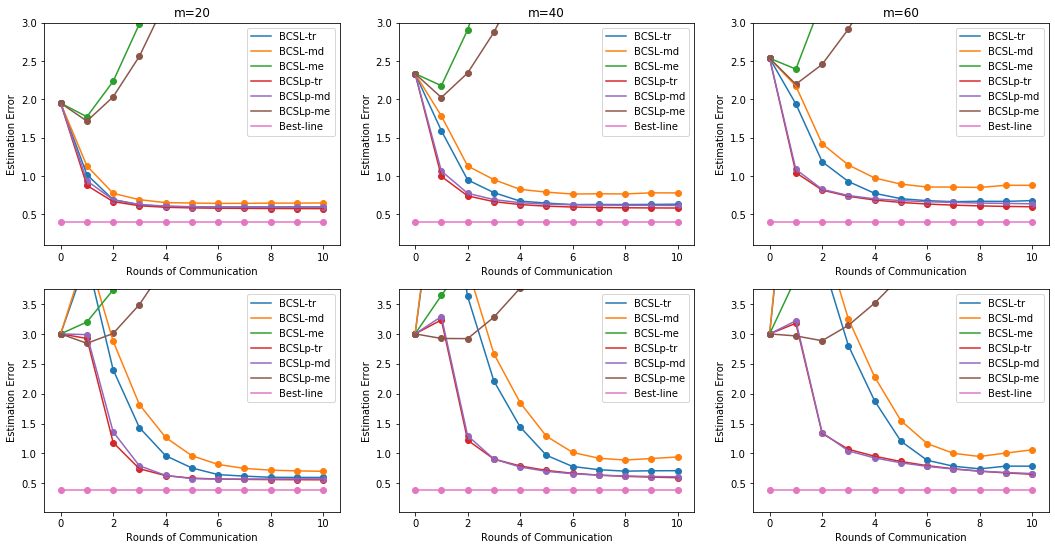
In the distributed learning, we split the whole dataset into each worker machine. According to the regimes “large nn”, “moderate nn” and “small nn”, we set the local sample size and the number of machines as (n,m)=(900,20)(n,m)=(900,20), (450,40)(450,40) and (300,60)(300,60) respectively. For our BCLS and BCLSp algorithms, we need to simulate the Byzantine failures. The αm\alpha m worker machines are randomly chosen to be Byzantine, and one of the rest work machines as the 1st worker machine. In the experiments, we set α=20%\alpha=20\%. In the coordinate-wise trimmed mean, set β=20%\beta=20\%. For evaluating the effect of initialization on the convergence, we respectively take 𝜽0=𝟎{\mbox{\boldmath${\theta}$}}_{0}={\mbox{\boldmath${0}$}}, and 𝜽¯\bar{{\mbox{\boldmath${\theta}$}}} which is the local estimator based on the data of the 1st machine. They are referred to “zero initialization” and “good initialization”, respectively.

We implement Algorithms BCLS and BCLSp based on median, trimmed mean and mean for aggregating all local gradients, which are called BCLS-md, BCLS-tr, BCLS-me, BCLSp-md, BCLSp-tr and BCLSp-me, respectively. In the first experiment, we choose g()=0g(\cdot)=0. The optimizations are carried out by mini batch stochastic gradient descent in the above algorithms. The estimation error 𝜽t𝜽2\|{\mbox{\boldmath${\theta}$}}_{t}-{\mbox{\boldmath${\theta}$}}^{*}\|_{2} is used to measure the performance of these different algorithms based on the 50 simulation replications.

Figure 1 shows how the estimation errors evolve with iterations for the case of p=100p=100 fixed. We find that our algorithms (BCLS-tr, BCLS-md, BCLSp-tr and BCLSp-md) converge reapidly in all scenarios, but the mean methods (BCLS-me and BCLSp-me) do not converge at all. Our algorithms almost converge after 2 iterations and do not require good initialization, which are in line with our theoretical results. This implies that our algorithms are robust against Byzantine failures, but the mean methods can’t tolerate such failures. In addition, our proposed Algorithm BCLSp is more robust and stable than Algorithm BCLS, especially for large mm. Note that large mm implies the more Byzantine worker machines. The embedding of the proximal technique in Algorithm BCLSp adds strict convex quadratic regularization, which leads to better performance.

Refer to caption
Figure 1: Impacts of local sample and initialization on convergence of algorithms for the fixed p=100p=100. The xx-axis is the number of iterations or the rounds of communications, and yy-axis is the estimation error 𝜽t𝜽2\|{\mbox{\boldmath${\theta}$}}_{t}-{\mbox{\boldmath${\theta}$}}^{*}\|_{2}. The “Best-line” shows the error of the minimizer of the overall loss function. Top panel uses 𝜽¯\boldsymbol{\bar{\theta}} as the initial value (“good initialization”) and bottom uses 𝟎\boldsymbol{0} as the initial value (“zero initialization”).

Next, we use the distributed logistic regression model (5.1) with sparsity. The experiment is used to validate the efficiency of our algorithms in the presence of a nonsmooth penalty. In the simulation, we still set the total sample size N=18000N=18000, but the dimensionality of 𝜽{\mbox{\boldmath${\theta}$}}^{*} is fixed to p=1000p=1000; the covariate vector 𝒖ij{\mbox{\boldmath${u}$}}_{ij} is i.i.d. N(𝟎,𝑰p)N({\mbox{\boldmath${0}$}},{\mbox{\boldmath${I}$}}_{p}) and 𝜽=(𝒗10T,𝟎991T)T1001{\mbox{\boldmath${\theta}$}}^{*}=({\mbox{\boldmath${v}$}}_{10}^{T},{\mbox{\boldmath${0}$}}_{991}^{T})^{T}\in\mathbb{R}^{1001} with 𝒗10N(𝟎10,𝑰10){\mbox{\boldmath${v}$}}_{10}\sim N({\mbox{\boldmath${0}$}}_{10},{\mbox{\boldmath${I}$}}_{10}). The 2\ell_{2}-norm of 𝜽{\mbox{\boldmath${\theta}$}}^{*} is constrained to 3. We choose the penalty function g(𝜽)=γ𝜽1g({\mbox{\boldmath${\theta}$}})=\gamma\|\boldsymbol{\theta}\|_{1} with γ=0.2logpN\gamma=0.2\sqrt{{\frac{\log{p}}{N}}} so that the nonzeros of 𝜽{\mbox{\boldmath${\theta}$}}^{*} can be recovers accurately by the regularized maximum likelihood estimation over the whole dataset. As in the first experiment, we set (n,m)=(900,20)(n,m)=(900,20), (450,40)(450,40) and (300,60)(300,60), α=20%\alpha=20\%, β=20%\beta=20\%, 𝜽0=𝟎{\mbox{\boldmath${\theta}$}}_{0}={\mbox{\boldmath${0}$}} (“zero initialization”) and 𝜽¯\bar{{\mbox{\boldmath${\theta}$}}} (“good initialization”). The 𝜽¯\bar{{\mbox{\boldmath${\theta}$}}} is the local estimator based on the dataset of the 1st machine. In the Algorithm BCLSp, the penalty parameters are selected appropriately for the cases of “good initialization” and “zero initialization”, respectively. The optimizations are carried out by mini batch stochastic sub-gradient descent in the algorithms. All the results are average values of 20 independent runs.

Figure 2 presents the performance of our algorithms and the mean aggregate method (BCLS-me and BCLSp-me). With proper regularization, our algorithms still work well whether the initial value is “good” or “bad”. The mean aggregate methods (BCLS-me and BCLSp-me) fail to converge. For this nonsmooth problem, Algorithms BCLSp-tr and BCLSp-md are more robust than Algorithms BCLS-tr and BCLS-md, and start to converge after just 2 rounds of communication, specially for the case of “good initialization”.

Refer to caption
Figure 2: Performance of the nonsmooth regularized algorithms for the distributed sparse logistic regression. The xx-axis is the number of iterations or the rounds of communications, and yy-axis is the estimation error 𝜽t𝜽2\|{\mbox{\boldmath${\theta}$}}_{t}-{\mbox{\boldmath${\theta}$}}^{*}\|_{2}. The “Best-line” shows the error of the minimizer of the overall loss function. Top panel uses 𝜽¯\boldsymbol{\bar{\theta}} as the initial value (“good initialization”) and bottom uses 𝟎\boldsymbol{0} as the initial value (“zero initialization”).

Here, we summarize the above simulations to highlight several outstanding advantages of our algorithms.

(1) Our proposed Byzantine-Robust CSL distributed learning algorithm (BCLS-md, BCLSp-tr) and Byzantine-Robust CSL-proximal distributed learning algorithm (BCLSp-md and BCLSp-tr) can indeed defend against Byzantine failures.

(2) Our proposed algorithms converge rapidly, usually with several rounds of communication, and do not require good initialization; these are consistent with our statistical theory.

(3) The Algorithms BCLSp-md and BCLSp-tr are more robust than Algorithms BCLS-md and BCLS-tr, due to add strict convex quadratic regularization by embedding proximal technique into Algorithm BCLSp.

5.2 Real data

In the subsection, we further assess the performance of our proposed algorithms by a real data example. We choose Spambase dataset from the UC Irvine Machine Learning Repository (Dua and Graff, 2017). The collection of Span e-mails in Spambase dataset come from their postmaster and individuals who had filed spam, and the collection of non-spam e-mails came from filed work and personal e-mails. Number of instances (total sample) is 4600, and Number of Attributes (features) is 57 based on their word frequencies and other characteristics. The goal is to use distributed logistic regression to construct a personalized spam filter that distinguishes spam emails from normal ones. In the experiment, randomly selecting 1000 instances as the testing set and the rest of 3600 instances as the training set; split the training set to each worker machine according to (n,m)=(180,20)(n,m)=(180,20) (“small mm”), (120,30)(120,30) (“moderate mm”) and (90,40)(90,40) (“large mm”), respectively; set α=20%\alpha=20\% for the fraction of Byzantine worker machines and β=20%\beta=20\% for the BCLS-tr and BCLSp-tr algorithms. We use classification errors on the test set as the evaluation criteria.

Figure 3 shows the average performance of the 6 algorithms mentioned in Subsection 5.1. We find that the testing errors of our algorithms are very low. It implies our algorithms can accurately filter spam and non spam, even for more Byzantine worker machines (“large mm”). But the filters based on Algorithms BCLS-me and BCLSp-me fail. These results are consistent with the ones of simulation experiments. Totally, the experiments on the real data also support our theoretical findings.

Refer to caption
Figure 3: Experiments on Spambase dataset. The xx-axis is the number of iterations or the rounds of communications, and yy-axis is testing error (prediction accuracy). The “Best-line” show the error of the filter based on all of the training dataset.

Acknowledgments

This work is partially supported by Chinese National Social Science Fund (No. 19BTJ034).

References

  • Blanchard et al. (2017) Blanchard P, El Mhamdi EM, Guerraoui R, Stainer J. Machine learning with adversaries: Byzantine tolerant gradient descent. Proceedings of NIPS 2017;:118–28.
  • Chen et al. (2017) Chen Y, Su L, Xu J. Distributed statistical machine learning in adversarial settings: Byzantine gradient descent. Proc ACM Meas Anal Comput Syst 2017;1:1–25.
  • Dua and Graff (2017) Dua D, Graff C. Uci machine learning repository 2017;URL: https://archive.ics.uci.edu/ml/datasets/Spambase.
  • Fan et al. (2019) Fan J, Guo Y, Wang K. Communication-efficient accurate statistical estimation. arXiv preprint 2019;arXiv:1906.04870.
  • Jordan et al. (2019) Jordan MI, Lee JD, Yang Y. Communication-efficient distributed statistical inference. Journal of the American Statistical Association 2019;114(526):668–81.
  • Konečnỳ et al. (2016) Konečnỳ J, McMahan HB, Yu FX, Richtárik P, Suresh AT, Bacon D. Federated learning: Strategies for improving communication efficiency. arXiv preprint 2016;arXiv:1610.05492.
  • Lee et al. (2017) Lee JD, Lin Q, Ma T, Yang T. Distributed stochastic variance reduced gradient methods by sampling extra data with replacement. Journal of Machine Learning Research 2017;18:4404–46.
  • Mei et al. (2018) Mei S, Bai Y, Montanari A. The landscape of empirical risk for nonconvex losses. The Annals of Statistics 2018;46:2747–74.
  • Minsker (2015) Minsker S. Geometric median and robust estimation in banach spaces. Bernoulli 2015;21(4):2308–35.
  • Nesterov (2004) Nesterov Y. Introductory Letures on Convex Optimization: A Basic Course. New York: Springer Science and Business Media, 2004.
  • Parikh and Boyd (2014) Parikh N, Boyd S. Proximal algorithms. Foundations and Trends® in Optimization 2014;1:127–239.
  • Rockafellar (1976) Rockafellar RT. Monotone operators and the proximal point algorithm. SIAM Journal on control and optimization 1976;14:877–98.
  • Shamir et al. (2014) Shamir O, Srebro N, Zhang T. Communication efficient distributed optimization using an approximate newton-type method. Proceedings of the 31st International Conference on Machine Learning 2014;:1000–8.
  • Su and Xu (2018) Su L, Xu J. Securing distributed machine learning in high dimensions. arxiv Preprint 2018;arXiv:1804.10140.
  • Tibshirani (1996) Tibshirani R. Regression shrinkage and selection via the lasso. Journal of the Royal Statistical Society Series B (Methodological) 1996;58(1):267–88.
  • Vempaty et al. (2013) Vempaty A, Tong L, Varshney PK. Distributed inference with byzantine data: State-of-the-art review on data falsification attacks. IEEE Signal Processing Magazine 2013;30(5):65–75.
  • Wang et al. (2017a) Wang J, Kolar M, Srebro N, Zhang T. Efficient distributed learning with sparsity. Proceedings of Machine Learning Research, PMLR 2017a;70:3636–45.
  • Wang et al. (2017b) Wang J, Wang W, Srebro N. Memory and communication efficient distributed stochastic optimization with minibatch prox. Proceedings of the 2017 Conference on Learning Theory, PMLR 2017b;65:1882–919.
  • Wu et al. (2019) Wu Z, Ling Q, Chen T, Giannakis GB. Federated variance-reduced stochastic gradient descent with robustness to byzantine attacks. arXiv Preprint 2019;arXiv:1912.12716v1.
  • Xie et al. (2018) Xie C, Koyejo O, Gupta I. Generalized byzantine-tolerant sgd. arXiv Preprint 2018;arXiv:1802.10116.
  • Yang et al. (2019) Yang Z, Gang A, Bajwa WU. Adversary-resilient inference and machine learning: From distributed to decentralized. arXiv Preprint 2019;arXiv:1908.08649.
  • Yin et al. (2018) Yin D, Chen Y, Ramchandran K, Bartlett P. Byzantine-robust distributed learning: towards optimal statistical rates. Proceedings of the 35th International Conference on Machine Learning, PMLR 2018;80:5650–9.
  • Zhang et al. (2015) Zhang Y, Duchi J, Wainwright M. Divide and conquer kernel ridge regression: A distributed algorithm with minimax optimal rates. The Journal of Machine Learning Research 2015;16:3299–340.
  • Zhang et al. (2013) Zhang Y, Duchi JC, Wainwright MJ. Communication-efficient algorithms for statistical optimization. Journal of Machine Learning Research 2013;14:3321–63.

Appendix A

A.1 Proof of Theorems 3.1 and 3.2

Proof of Theorem 3.1: Define

φ(𝝃)=argmin𝜽{f1(𝜽)f1(𝝃)𝒉(𝝃),𝜽+g(𝜽)}.\varphi({\mbox{\boldmath${\xi}$}})=\mathrm{argmin}_{\mbox{\boldmath${\theta}$}}\left\{f_{1}({\mbox{\boldmath${\theta}$}})-\langle{\mbox{\boldmath${\nabla}$}}f_{1}({\mbox{\boldmath${\xi}$}})-{\mbox{\boldmath${h}$}}({\mbox{\boldmath${\xi}$}}),{\mbox{\boldmath${\theta}$}}\rangle+g({\mbox{\boldmath${\theta}$}})\right\}.

Obviously, 𝜽t+1=φ(𝜽t){\mbox{\boldmath${\theta}$}}_{t+1}=\varphi({\mbox{\boldmath${\theta}$}}_{t}). By Theorem 8 in Yin et al. (2018) and the law of large numbers, for 𝝃𝚯{\mbox{\boldmath${\xi}$}}\in{\mbox{\boldmath${\Theta}$}}, we have

f1(𝜽)f1(𝝃)𝒉(𝝃),𝜽+g(𝜽)\displaystyle f_{1}({\mbox{\boldmath${\theta}$}})-\langle{\mbox{\boldmath${\nabla}$}}f_{1}({\mbox{\boldmath${\xi}$}})-{\mbox{\boldmath${h}$}}({\mbox{\boldmath${\xi}$}}),{\mbox{\boldmath${\theta}$}}\rangle+g({\mbox{\boldmath${\theta}$}}) (A.1)
=\displaystyle= {f1(𝜽)f1(𝝃)f(𝝃),𝜽+g(𝜽)}+[𝒉(𝝃)F(𝝃)]+[F(𝝃)f(𝝃)]\displaystyle\left\{f_{1}({\mbox{\boldmath${\theta}$}})-\langle{\mbox{\boldmath${\nabla}$}}f_{1}({\mbox{\boldmath${\xi}$}})-\nabla f({\mbox{\boldmath${\xi}$}}),{\mbox{\boldmath${\theta}$}}\rangle+g({\mbox{\boldmath${\theta}$}})\right\}+[{\mbox{\boldmath${h}$}}({\mbox{\boldmath${\xi}$}})-\nabla F({\mbox{\boldmath${\xi}$}})]+[\nabla F({\mbox{\boldmath${\xi}$}})-\nabla f({\mbox{\boldmath${\xi}$}})]
=\displaystyle= {f1(𝜽)f1(𝝃)f(𝝃),𝜽+g(𝜽)}+op(1).\displaystyle\left\{f_{1}({\mbox{\boldmath${\theta}$}})-\langle{\mbox{\boldmath${\nabla}$}}f_{1}({\mbox{\boldmath${\xi}$}})-\nabla f({\mbox{\boldmath${\xi}$}}),{\mbox{\boldmath${\theta}$}}\rangle+g({\mbox{\boldmath${\theta}$}})\right\}+o_{p}(1).

Therefore, φ(𝜽^)=𝜽^+op(1)\varphi(\hat{{\mbox{\boldmath${\theta}$}}})=\hat{{\mbox{\boldmath${\theta}$}}}+o_{p}(1), that is, 𝜽^\hat{{\mbox{\boldmath${\theta}$}}} is a asymptotic fixed point of φ()\varphi(\cdot) . For the fixed 𝜽B(𝜽^,R){\mbox{\boldmath${\theta}$}}\in B(\hat{{\mbox{\boldmath${\theta}$}}},R), by the first order condition of φ(𝜽)\varphi({\mbox{\boldmath${\theta}$}}), we have that

f1(𝜽)𝒉(𝜽){f1(φ(𝜽))+g(φ(𝜽))}.\nabla f_{1}({\mbox{\boldmath${\theta}$}})-{\mbox{\boldmath${h}$}}({\mbox{\boldmath${\theta}$}})\in\partial\left\{f_{1}(\varphi({\mbox{\boldmath${\theta}$}}))+g(\varphi({\mbox{\boldmath${\theta}$}}))\right\}. (A.2)

Further,

f1(𝜽^)𝒉(𝜽^){f1(𝜽^)+g(𝜽^)},\nabla f_{1}(\hat{{\mbox{\boldmath${\theta}$}}})-{\mbox{\boldmath${h}$}}(\hat{{\mbox{\boldmath${\theta}$}}})\in\partial\left\{f_{1}(\hat{{\mbox{\boldmath${\theta}$}}})+g(\hat{{\mbox{\boldmath${\theta}$}}})\right\}, (A.3)

by using the fact φ(𝜽^)=𝜽^\varphi(\hat{{\mbox{\boldmath${\theta}$}}})=\hat{{\mbox{\boldmath${\theta}$}}}.

By the Taylor expansion, Assumption 3.4 and Theorem 8 in Yin et al. (2018), with probability at least 14p(1+n(m+1)L~D)p1-\frac{4p}{(1+n(m+1)\tilde{L}D)^{p}}, we have

[f1(𝜽)h(𝜽)][f1(𝜽^)h(𝜽^)]2\displaystyle\|[\nabla f_{1}({\mbox{\boldmath${\theta}$}})-h({\mbox{\boldmath${\theta}$}})]-[\nabla f_{1}(\hat{{\mbox{\boldmath${\theta}$}}})-h(\hat{{\mbox{\boldmath${\theta}$}}})]\|_{2} (A.4)
\displaystyle\leq [f1(𝜽)F(𝜽)][f1(𝜽^)F(𝜽^)]2+[F(𝜽)h(𝜽)][F(𝜽^)h(𝜽^)]2\displaystyle\|[\nabla f_{1}({\mbox{\boldmath${\theta}$}})-\nabla F({\mbox{\boldmath${\theta}$}})]-[\nabla f_{1}(\hat{{\mbox{\boldmath${\theta}$}}})-\nabla F(\hat{{\mbox{\boldmath${\theta}$}}})]\|_{2}+\|[\nabla F({\mbox{\boldmath${\theta}$}})-h({\mbox{\boldmath${\theta}$}})]-[\nabla F(\hat{{\mbox{\boldmath${\theta}$}}})-h(\hat{{\mbox{\boldmath${\theta}$}}})]\|_{2}
\displaystyle\leq [f1(𝜽)f1(𝜽^)][F(𝜽)F(𝜽^)]2+2Δnmα\displaystyle\|[\nabla f_{1}({\mbox{\boldmath${\theta}$}})-\nabla f_{1}(\hat{{\mbox{\boldmath${\theta}$}}})]-[\nabla F({\mbox{\boldmath${\theta}$}})-\nabla F(\hat{{\mbox{\boldmath${\theta}$}}})]\|_{2}+2\Delta_{nm\alpha}
=\displaystyle= 01(2f1[(1t)𝜽^+t𝜽]2F[(1t)𝜽^+t𝜽])(𝜽𝜽^)𝑑t2+2Δnmα\displaystyle\left\|\int_{0}^{1}\left(\nabla^{2}f_{1}[(1-t)\hat{{\mbox{\boldmath${\theta}$}}}+t{\mbox{\boldmath${\theta}$}}]-\nabla^{2}F[(1-t)\hat{{\mbox{\boldmath${\theta}$}}}+t{\mbox{\boldmath${\theta}$}}]\right)({\mbox{\boldmath${\theta}$}}-\hat{{\mbox{\boldmath${\theta}$}}})dt\right\|_{2}+2\Delta_{nm\alpha}
\displaystyle\leq supζB(𝜽^,R)2f1(ζ)2F(ζ)2𝜽𝜽^2+2Δnmα\displaystyle\sup_{\zeta\in B(\hat{{\mbox{\boldmath${\theta}$}}},R)}\|\nabla^{2}f_{1}(\zeta)-\nabla^{2}F(\zeta)\|_{2}\|{\mbox{\boldmath${\theta}$}}-\hat{{\mbox{\boldmath${\theta}$}}}\|_{2}+2\Delta_{nm\alpha}
\displaystyle\leq δ𝜽𝜽^2+2ΔnmαδR+2Δnmα=(δ+2Δnmα/R)R<ρR.\displaystyle\delta\|{\mbox{\boldmath${\theta}$}}-\hat{{\mbox{\boldmath${\theta}$}}}\|_{2}+2\Delta_{nm\alpha}\leq\delta R+2\Delta_{nm\alpha}=(\delta+2\Delta_{nm\alpha}/R)R<\rho R.

Next, we will show that under (A.2)-(A.4), we have

φ(𝜽)𝜽^2[f1(𝜽)h(𝜽)][f1(𝜽^)h(𝜽^)]2/ρ.\|\varphi({\mbox{\boldmath${\theta}$}})-\hat{{\mbox{\boldmath${\theta}$}}}\|_{2}\leq\left\|[\nabla f_{1}({\mbox{\boldmath${\theta}$}})-h({\mbox{\boldmath${\theta}$}})]-[\nabla f_{1}(\hat{{\mbox{\boldmath${\theta}$}}})-h(\hat{{\mbox{\boldmath${\theta}$}}})]\right\|_{2}/\rho. (A.5)

If we know φ(𝜽)𝜽^2R\|\varphi({\mbox{\boldmath${\theta}$}})-\hat{{\mbox{\boldmath${\theta}$}}}\|_{2}\leq R in advance, then

ρφ(𝜽)𝜽^22\displaystyle\rho\|\varphi({\mbox{\boldmath${\theta}$}})-\hat{{\mbox{\boldmath${\theta}$}}}\|_{2}^{2} \displaystyle\leq [f1(𝜽)h(𝜽)][f1(𝜽^)h(𝜽^)],φ(θ)𝜽^\displaystyle\left\langle[\nabla f_{1}({\mbox{\boldmath${\theta}$}})-h({\mbox{\boldmath${\theta}$}})]-[\nabla f_{1}(\hat{{\mbox{\boldmath${\theta}$}}})-h(\hat{{\mbox{\boldmath${\theta}$}}})],\varphi(\theta)-\hat{{\mbox{\boldmath${\theta}$}}}\right\rangle
\displaystyle\leq [f1(𝜽)h(𝜽)][f1(𝜽^)h(𝜽^)]2φ(θ)𝜽^2.\displaystyle\|[\nabla f_{1}({\mbox{\boldmath${\theta}$}})-h({\mbox{\boldmath${\theta}$}})]-[\nabla f_{1}(\hat{{\mbox{\boldmath${\theta}$}}})-h(\hat{{\mbox{\boldmath${\theta}$}}})]\|_{2}\|\varphi(\theta)-\hat{{\mbox{\boldmath${\theta}$}}}\|_{2}.

Here the 1st inequality follows from the ρ\rho-strong convex in B(𝜽^,R)B(\hat{{\mbox{\boldmath${\theta}$}}},R) of f1+gf_{1}+g and (A.2)-(A.3); the 2nd step uses the Cauchy-Schwarz inequality. Then, we obtain the desired result (A.5). Suppose on the contrary that φ(𝜽)𝜽^2>R\|\varphi({\mbox{\boldmath${\theta}$}})-\hat{{\mbox{\boldmath${\theta}$}}}\|_{2}>R. We use reduction to absurdity. Define φ(𝜽¯)=𝜽^+R(φ(𝜽)𝜽^)/φ(𝜽)𝜽^2\varphi(\bar{{\mbox{\boldmath${\theta}$}}})=\hat{{\mbox{\boldmath${\theta}$}}}+R(\varphi({\mbox{\boldmath${\theta}$}})-\hat{{\mbox{\boldmath${\theta}$}}})/\|\varphi({\mbox{\boldmath${\theta}$}})-\hat{{\mbox{\boldmath${\theta}$}}}\|_{2}. Obviously, φ(𝜽¯)𝜽^2=R\|\varphi(\bar{{\mbox{\boldmath${\theta}$}}})-\hat{{\mbox{\boldmath${\theta}$}}}\|_{2}=R. By the strong convexity of f1+gf_{1}+g in B(𝜽^,R)B(\hat{{\mbox{\boldmath${\theta}$}}},R) and (A.2)-(A.3) again,

[f1(𝜽¯)h(𝜽¯)][f1(𝜽^)h(𝜽^)],φ(𝜽¯)𝜽^ρφ(𝜽¯)𝜽^22;\left\langle[f_{1}(\bar{{\mbox{\boldmath${\theta}$}}})-h(\bar{{\mbox{\boldmath${\theta}$}}})]-[f_{1}(\hat{{\mbox{\boldmath${\theta}$}}})-h(\hat{{\mbox{\boldmath${\theta}$}}})],\varphi(\bar{{\mbox{\boldmath${\theta}$}}})-\hat{{\mbox{\boldmath${\theta}$}}}\right\rangle\geq\rho\|\varphi(\bar{{\mbox{\boldmath${\theta}$}}})-\hat{{\mbox{\boldmath${\theta}$}}}\|_{2}^{2}; (A.6)

Notice that

φ(𝜽¯)𝜽^=Rφ(𝜽)𝜽^2R(φ(𝜽)φ(𝜽¯)).\varphi(\bar{{\mbox{\boldmath${\theta}$}}})-\hat{{\mbox{\boldmath${\theta}$}}}=\frac{R}{\|\varphi({\mbox{\boldmath${\theta}$}})-\hat{{\mbox{\boldmath${\theta}$}}}\|_{2}-R}(\varphi({\mbox{\boldmath${\theta}$}})-\varphi(\bar{{\mbox{\boldmath${\theta}$}}})).

Thus, by the convexity of f1+gf_{1}+g and (A.2), we always have

[f1(𝜽)h(𝜽)][f1(𝜽¯)h(𝜽¯)],φ(𝜽¯)𝜽^\displaystyle\left\langle[f_{1}({{\mbox{\boldmath${\theta}$}}})-h({{\mbox{\boldmath${\theta}$}}})]-[f_{1}(\bar{{\mbox{\boldmath${\theta}$}}})-h(\bar{{\mbox{\boldmath${\theta}$}}})],\varphi(\bar{{\mbox{\boldmath${\theta}$}}})-\hat{{\mbox{\boldmath${\theta}$}}}\right\rangle (A.7)
=\displaystyle= Rφ(𝜽)𝜽^2R[f1(𝜽)h(𝜽)][f1(𝜽¯)h(𝜽¯)],φ(𝜽)φ(𝜽¯)0,\displaystyle\frac{R}{\|\varphi({\mbox{\boldmath${\theta}$}})-\hat{{\mbox{\boldmath${\theta}$}}}\|_{2}-R}\left\langle[f_{1}({{\mbox{\boldmath${\theta}$}}})-h({{\mbox{\boldmath${\theta}$}}})]-[f_{1}(\bar{{\mbox{\boldmath${\theta}$}}})-h(\bar{{\mbox{\boldmath${\theta}$}}})],\varphi({\mbox{\boldmath${\theta}$}})-\varphi(\bar{{\mbox{\boldmath${\theta}$}}})\right\rangle\geq 0,

for any 𝜽¯B(𝜽^,R)\bar{{\mbox{\boldmath${\theta}$}}}\in B(\hat{{\mbox{\boldmath${\theta}$}}},R). Summing up the (A.6), and by (A.7) and Cauchy-Schwarz inequality, one gets

ρφ(𝜽¯)𝜽^22\displaystyle\rho\|\varphi(\bar{{\mbox{\boldmath${\theta}$}}})-\hat{{\mbox{\boldmath${\theta}$}}}\|_{2}^{2} \displaystyle\leq [f1(𝜽)h(𝜽)][f1(𝜽^)h(𝜽^)],φ(𝜽¯)𝜽^\displaystyle\left\langle[f_{1}({{\mbox{\boldmath${\theta}$}}})-h({{\mbox{\boldmath${\theta}$}}})]-[f_{1}(\hat{{\mbox{\boldmath${\theta}$}}})-h(\hat{{\mbox{\boldmath${\theta}$}}})],\varphi(\bar{{\mbox{\boldmath${\theta}$}}})-\hat{{\mbox{\boldmath${\theta}$}}}\right\rangle
\displaystyle\leq [f1(𝜽)h(𝜽)][f1(𝜽^)h(𝜽^)]2φ(𝜽¯)𝜽^2.\displaystyle\|[f_{1}({{\mbox{\boldmath${\theta}$}}})-h({{\mbox{\boldmath${\theta}$}}})]-[f_{1}(\hat{{\mbox{\boldmath${\theta}$}}})-h(\hat{{\mbox{\boldmath${\theta}$}}})]\|_{2}\|\varphi(\bar{{\mbox{\boldmath${\theta}$}}})-\hat{{\mbox{\boldmath${\theta}$}}}\|_{2}.

Thus, [f1(𝜽)h(𝜽)][f1(𝜽^)h(𝜽^)]2ρφ(𝜽¯)𝜽^2=ρR\|[f_{1}({{\mbox{\boldmath${\theta}$}}})-h({{\mbox{\boldmath${\theta}$}}})]-[f_{1}(\hat{{\mbox{\boldmath${\theta}$}}})-h(\hat{{\mbox{\boldmath${\theta}$}}})]\|_{2}\geq\rho\|\varphi(\bar{{\mbox{\boldmath${\theta}$}}})-\hat{{\mbox{\boldmath${\theta}$}}}\|_{2}=\rho R, which contradicts (A.4). Therefore, we must have only φ(𝜽)𝜽^2R\|\varphi({\mbox{\boldmath${\theta}$}})-\hat{{\mbox{\boldmath${\theta}$}}}\|_{2}\leq R. And then (A.5) holds. Together with (A.4), with probability at least 14p(1+n(m+1)L~D)p1-\frac{4p}{(1+n(m+1)\tilde{L}D)^{p}}, we have

φ(𝜽)𝜽^2δρ𝜽𝜽^2+2ρΔnmα.\|\varphi({\mbox{\boldmath${\theta}$}})-\hat{{\mbox{\boldmath${\theta}$}}}\|_{2}\leq\frac{\delta}{\rho}\|{\mbox{\boldmath${\theta}$}}-\hat{{\mbox{\boldmath${\theta}$}}}\|_{2}+\frac{2}{\rho}\Delta_{nm\alpha}.

Take 𝜽=𝜽t{\mbox{\boldmath${\theta}$}}={\mbox{\boldmath${\theta}$}}_{t}, then φ(𝜽t)=𝜽t+1\varphi({\mbox{\boldmath${\theta}$}}_{t})={\mbox{\boldmath${\theta}$}}_{t+1}. We complete the proof of Theorem 3.1.

Proof of Theorem 3.2: The proof is essentially the same as the proof of Theorem 3.1, except that the analysis of coordinate-wise trimmed mean of means estimator of the population gradients, which can be found in Yin et al. (2018), is different one of coordinate-wise median.

A.2 Proof of Theorems 3.3 and 3.4

Theorems 3.3 and 3.4 are the special cases of Theorem 4.3 (ii) by taking λ=0\lambda=0. See subsection A. for the proofs of Theorem 4.3.

A.3 Proofs of Theorems 4.1, 4.2 and Corollary 4.1

Proof of Theorem 4.1: Under the conditions of Theorem 4.1, if 0<𝜽t𝜽^2<R/20<\|{\mbox{\boldmath${\theta}$}}_{t}-\hat{{\mbox{\boldmath${\theta}$}}}\|_{2}<R/2, then (4.3) holds. Then Theorem 4.1 can directly follow from the result and induction. Below we prove the result.

Recall that 𝜽^=argmin𝜽(f(𝜽)+g(𝜽))\hat{{\mbox{\boldmath${\theta}$}}}=\mathrm{argmin}_{\mbox{\boldmath${\theta}$}}(f({\mbox{\boldmath${\theta}$}})+g({\mbox{\boldmath${\theta}$}})). Denote 𝜽t+=proxλ1(f+g)(𝜽t){\mbox{\boldmath${\theta}$}}_{t}^{+}=\mathrm{prox}_{\lambda^{-1}(f+g)}({\mbox{\boldmath${\theta}$}}_{t}). By the triangle inequality,

𝜽t+1𝜽^2𝜽t+1𝜽t+2+𝜽t+𝜽^2.\|{\mbox{\boldmath${\theta}$}}_{t+1}-\hat{{\mbox{\boldmath${\theta}$}}}\|_{2}\leq\|{\mbox{\boldmath${\theta}$}}_{t+1}-{\mbox{\boldmath${\theta}$}}_{t}^{+}\|_{2}+\|{\mbox{\boldmath${\theta}$}}_{t}^{+}-\hat{{\mbox{\boldmath${\theta}$}}}\|_{2}. (A.8)

For the first term on the right of (A.8), 𝜽t+1𝜽t+2\|{\mbox{\boldmath${\theta}$}}_{t+1}-{\mbox{\boldmath${\theta}$}}_{t}^{+}\|_{2}, we can obtain its contracting optimization errors by Theorem 3.1, taking g(𝜽)g({\mbox{\boldmath${\theta}$}}) in Algorithm 1 as g~(𝜽)=g(𝜽)+λ2𝜽𝜽t22\tilde{g}({\mbox{\boldmath${\theta}$}})=g({\mbox{\boldmath${\theta}$}})+\frac{\lambda}{2}\|{\mbox{\boldmath${\theta}$}}-{\mbox{\boldmath${\theta}$}}_{t}\|_{2}^{2}. Thus, 𝜽t+=argmin𝜽{f(𝜽)+g~(𝜽)}{\mbox{\boldmath${\theta}$}}_{t}^{+}=\mathrm{argmin}_{\mbox{\boldmath${\theta}$}}\left\{f({\mbox{\boldmath${\theta}$}})+\tilde{g}({\mbox{\boldmath${\theta}$}})\right\}. Together with (4.2), 𝜽t+1{\mbox{\boldmath${\theta}$}}_{t+1} is regarded as the first iterate of Algorithm 1 initialized at 𝜽t{\mbox{\boldmath${\theta}$}}_{t} for obtaining 𝜽t+{\mbox{\boldmath${\theta}$}}_{t}^{+}. Here, 𝜽t+{\mbox{\boldmath${\theta}$}}_{t}^{+} is similar to 𝜽^\hat{{\mbox{\boldmath${\theta}$}}} in Algorithm 1. Contrasting the assumptions of Theorem 3.1, we still need the following assertions:

(i) 𝜽tB(𝜽t+,R/2){\mbox{\boldmath${\theta}$}}_{t}\in B({\mbox{\boldmath${\theta}$}}_{t}^{+},R/2);

(ii) f+g~f+\tilde{g} is ρ+λ\rho+\lambda-strongly convex in B(𝜽t+,R/2)B({\mbox{\boldmath${\theta}$}}_{t}^{+},R/2);

(iii) 2f1(𝜽)2F(𝜽)2δ\|\nabla^{2}f_{1}({\mbox{\boldmath${\theta}$}})-\nabla^{2}F({\mbox{\boldmath${\theta}$}})\|_{2}\leq\delta, and 𝜽B(𝜽t+,R/2){\mbox{\boldmath${\theta}$}}\in B({\mbox{\boldmath${\theta}$}}_{t}^{+},R/2).

Let f~=f+g\tilde{f}=f+g. Notice that

𝜽^=proxλ1f~(𝜽^).\hat{{\mbox{\boldmath${\theta}$}}}=\mathrm{prox}_{\lambda^{-1}\tilde{f}}(\hat{{\mbox{\boldmath${\theta}$}}}). (A.9)

By the well-known “firm non-expansiveness” property of the proximal operation (Parikh and Boyd, 2014), we have

proxλ1f~(𝜽t)proxλ1f~(𝜽^)22𝜽t𝜽^,proxλ1f~(𝜽t)proxλ1f~(𝜽^).\left\|\mathrm{prox}_{\lambda^{-1}\tilde{f}}({\mbox{\boldmath${\theta}$}}_{t})-\mathrm{prox}_{\lambda^{-1}\tilde{f}}(\hat{{\mbox{\boldmath${\theta}$}}})\right\|_{2}^{2}\leq\left\langle{\mbox{\boldmath${\theta}$}}_{t}-\hat{{\mbox{\boldmath${\theta}$}}},\mathrm{prox}_{\lambda^{-1}\tilde{f}}({\mbox{\boldmath${\theta}$}}_{t})-\mathrm{prox}_{\lambda^{-1}\tilde{f}}(\hat{{\mbox{\boldmath${\theta}$}}})\right\rangle. (A.10)

From (A.9)-(A.10), we have 𝜽t+𝜽^2=proxλ1f~(𝜽t)𝜽^2𝜽t𝜽^2\|{\mbox{\boldmath${\theta}$}}_{t}^{+}-\hat{{\mbox{\boldmath${\theta}$}}}\|_{2}=\|\mathrm{prox}_{\lambda^{-1}\tilde{f}}({\mbox{\boldmath${\theta}$}}_{t})-\hat{{\mbox{\boldmath${\theta}$}}}\|_{2}\leq\|{\mbox{\boldmath${\theta}$}}_{t}-\hat{{\mbox{\boldmath${\theta}$}}}\|_{2}. So, the condition 𝜽t𝜽^2<R/2\|{\mbox{\boldmath${\theta}$}}_{t}-\hat{{\mbox{\boldmath${\theta}$}}}\|_{2}<R/2 implies B(𝜽t+,R/2)B(𝜽^,R)B({\mbox{\boldmath${\theta}$}}_{t}^{+},R/2)\subset B(\hat{{\mbox{\boldmath${\theta}$}}},R). Assumptions 3.3 and 3.4 imply (ii) and (iii) hold, respectively. In the other hand,

proxλ1f~(𝜽t)𝜽t22=[proxλ1f~(𝜽t)𝜽^][𝜽t𝜽^]22\displaystyle\left\|\mathrm{prox}_{\lambda^{-1}\tilde{f}}({\mbox{\boldmath${\theta}$}}_{t})-{\mbox{\boldmath${\theta}$}}_{t}\right\|_{2}^{2}=\left\|[\mathrm{prox}_{\lambda^{-1}\tilde{f}}({\mbox{\boldmath${\theta}$}}_{t})-\hat{{\mbox{\boldmath${\theta}$}}}]-[{\mbox{\boldmath${\theta}$}}_{t}-\hat{{\mbox{\boldmath${\theta}$}}}]\right\|_{2}^{2}
=\displaystyle= proxλ1f~(𝜽t)𝜽^22+𝜽t𝜽^222proxλ1f~(𝜽t)𝜽^,𝜽t𝜽^\displaystyle\left\|\mathrm{prox}_{\lambda^{-1}\tilde{f}}({\mbox{\boldmath${\theta}$}}_{t})-\hat{{\mbox{\boldmath${\theta}$}}}\right\|_{2}^{2}+\|{\mbox{\boldmath${\theta}$}}_{t}-\hat{{\mbox{\boldmath${\theta}$}}}\|_{2}^{2}-2\left\langle\mathrm{prox}_{\lambda^{-1}\tilde{f}}({\mbox{\boldmath${\theta}$}}_{t})-\hat{{\mbox{\boldmath${\theta}$}}},{\mbox{\boldmath${\theta}$}}_{t}-\hat{{\mbox{\boldmath${\theta}$}}}\right\rangle
\displaystyle\leq proxλ1f~(𝜽t)𝜽^22+𝜽t𝜽^222proxλ1f~(𝜽t)𝜽^22\displaystyle\left\|\mathrm{prox}_{\lambda^{-1}\tilde{f}}({\mbox{\boldmath${\theta}$}}_{t})-\hat{{\mbox{\boldmath${\theta}$}}}\right\|_{2}^{2}+\|{\mbox{\boldmath${\theta}$}}_{t}-\hat{{\mbox{\boldmath${\theta}$}}}\|_{2}^{2}-2\left\|\mathrm{prox}_{\lambda^{-1}\tilde{f}}({\mbox{\boldmath${\theta}$}}_{t})-\hat{{\mbox{\boldmath${\theta}$}}}\right\|_{2}^{2}
=\displaystyle= 𝜽t𝜽^22proxλ1f~(𝜽t)𝜽^22,\displaystyle\|{\mbox{\boldmath${\theta}$}}_{t}-\hat{{\mbox{\boldmath${\theta}$}}}\|_{2}^{2}-\left\|\mathrm{prox}_{\lambda^{-1}\tilde{f}}({\mbox{\boldmath${\theta}$}}_{t})-\hat{{\mbox{\boldmath${\theta}$}}}\right\|_{2}^{2},

that is,

𝜽t+𝜽t22𝜽t𝜽^22𝜽t+𝜽^22.\|{\mbox{\boldmath${\theta}$}}_{t}^{+}-{\mbox{\boldmath${\theta}$}}_{t}\|_{2}^{2}\leq\|{\mbox{\boldmath${\theta}$}}_{t}-\hat{{\mbox{\boldmath${\theta}$}}}\|_{2}^{2}-\|{\mbox{\boldmath${\theta}$}}_{t}^{+}-\hat{{\mbox{\boldmath${\theta}$}}}\|_{2}^{2}.

Further,

𝜽t+𝜽t2𝜽t𝜽^21𝜽t+𝜽^22/𝜽t𝜽^22,\|{\mbox{\boldmath${\theta}$}}_{t}^{+}-{\mbox{\boldmath${\theta}$}}_{t}\|_{2}\leq\|{\mbox{\boldmath${\theta}$}}_{t}-\hat{{\mbox{\boldmath${\theta}$}}}\|_{2}\sqrt{1-\|{\mbox{\boldmath${\theta}$}}_{t}^{+}-\hat{{\mbox{\boldmath${\theta}$}}}\|_{2}^{2}/\|{\mbox{\boldmath${\theta}$}}_{t}-\hat{{\mbox{\boldmath${\theta}$}}}\|_{2}^{2}}, (A.11)

which leads to 𝜽t+𝜽t2𝜽t𝜽^2<R/2\|{\mbox{\boldmath${\theta}$}}_{t}^{+}-{\mbox{\boldmath${\theta}$}}_{t}\|_{2}\leq\|{\mbox{\boldmath${\theta}$}}_{t}-\hat{{\mbox{\boldmath${\theta}$}}}\|_{2}<R/2. Therefore, (i) holds.

Based the above assertions and ρ+λ>δ+2Δnmα/R\rho+\lambda>\delta+2\Delta_{nm\alpha}/R by (δ+2R1Δnmαρ+λ)2<ρρ+2λ\left(\frac{\delta+2R^{-1}\Delta_{nm\alpha}}{\rho+\lambda}\right)^{2}<\frac{\rho}{\rho+2\lambda}, by Theorem 3.1, we have

𝜽t+1𝜽t+2δρ+λ𝜽t𝜽t+2+2ρ+λΔnmα.\|{\mbox{\boldmath${\theta}$}}_{t+1}-{\mbox{\boldmath${\theta}$}}_{t}^{+}\|_{2}\leq\frac{\delta}{\rho+\lambda}\|{\mbox{\boldmath${\theta}$}}_{t}-{\mbox{\boldmath${\theta}$}}_{t}^{+}\|_{2}+\frac{2}{\rho+\lambda}\Delta_{nm\alpha}. (A.12)

From (A.8), (A.11) and (A.12), we have

𝜽t+1𝜽^2\displaystyle\|{\mbox{\boldmath${\theta}$}}_{t+1}-\hat{{\mbox{\boldmath${\theta}$}}}\|_{2} \displaystyle\leq δρ+λ𝜽t𝜽t+2+2ρ+λΔnmα+𝜽t+𝜽^2\displaystyle\frac{\delta}{\rho+\lambda}\|{\mbox{\boldmath${\theta}$}}_{t}-{\mbox{\boldmath${\theta}$}}_{t}^{+}\|_{2}+\frac{2}{\rho+\lambda}\Delta_{nm\alpha}+\|{\mbox{\boldmath${\theta}$}}_{t}^{+}-\hat{{\mbox{\boldmath${\theta}$}}}\|_{2} (A.13)
\displaystyle\leq 𝜽t𝜽^2(δρ+λ1𝜽t+𝜽^22𝜽t𝜽^22+𝜽t+𝜽^2𝜽t𝜽^2)+2ρ+λΔnmα\displaystyle\|{\mbox{\boldmath${\theta}$}}_{t}-\hat{{\mbox{\boldmath${\theta}$}}}\|_{2}\left(\frac{\delta}{\rho+\lambda}\sqrt{1-\frac{\|{\mbox{\boldmath${\theta}$}}_{t}^{+}-\hat{{\mbox{\boldmath${\theta}$}}}\|_{2}^{2}}{\|{\mbox{\boldmath${\theta}$}}_{t}-\hat{{\mbox{\boldmath${\theta}$}}}\|_{2}^{2}}}+\frac{\|{\mbox{\boldmath${\theta}$}}_{t}^{+}-\hat{{\mbox{\boldmath${\theta}$}}}\|_{2}}{\|{\mbox{\boldmath${\theta}$}}_{t}-\hat{{\mbox{\boldmath${\theta}$}}}\|_{2}}\right)+\frac{2}{\rho+\lambda}\Delta_{nm\alpha}
=\displaystyle= 𝜽t𝜽^2κ(𝜽t+𝜽^2𝜽t𝜽^2)+2ρ+λΔnmα,\displaystyle\|{\mbox{\boldmath${\theta}$}}_{t}-\hat{{\mbox{\boldmath${\theta}$}}}\|_{2}\kappa\left(\frac{\|{\mbox{\boldmath${\theta}$}}_{t}^{+}-\hat{{\mbox{\boldmath${\theta}$}}}\|_{2}}{\|{\mbox{\boldmath${\theta}$}}_{t}-\hat{{\mbox{\boldmath${\theta}$}}}\|_{2}}\right)+\frac{2}{\rho+\lambda}\Delta_{nm\alpha},

where κ(u)=δρ+λ1u2+u\kappa(u)=\frac{\delta}{\rho+\lambda}\sqrt{1-u^{2}}+u.

Here, we will prove

𝜽t+𝜽^2𝜽t𝜽^2λρ+λ<1,\frac{\|{\mbox{\boldmath${\theta}$}}_{t}^{+}-\hat{{\mbox{\boldmath${\theta}$}}}\|_{2}}{\|{\mbox{\boldmath${\theta}$}}_{t}-\hat{{\mbox{\boldmath${\theta}$}}}\|_{2}}\leq\frac{\lambda}{\rho+\lambda}<1, (A.14)

which makes (A.13) valid. Indeed, on the hand, 𝜽t+𝜽^2𝜽t𝜽^2\|{\mbox{\boldmath${\theta}$}}_{t}^{+}-\hat{{\mbox{\boldmath${\theta}$}}}\|_{2}\leq\|{\mbox{\boldmath${\theta}$}}_{t}-\hat{{\mbox{\boldmath${\theta}$}}}\|_{2}; on the other hand, 𝜽^=argmin𝜽f~(𝜽)\hat{{\mbox{\boldmath${\theta}$}}}=\mathrm{argmin}_{\mbox{\boldmath${\theta}$}}\tilde{f}({\mbox{\boldmath${\theta}$}}) and 𝜽t+=argmin𝜽(f~(𝜽)+λ/2𝜽𝜽t22){\mbox{\boldmath${\theta}$}}_{t}^{+}=\mathrm{argmin}_{\mbox{\boldmath${\theta}$}}\left(\tilde{f}({\mbox{\boldmath${\theta}$}})+\lambda/2\|{\mbox{\boldmath${\theta}$}}-{\mbox{\boldmath${\theta}$}}_{t}\|_{2}^{2}\right) imply that 𝟎f~(𝜽^){\mbox{\boldmath${0}$}}\in\partial\tilde{f}(\hat{{\mbox{\boldmath${\theta}$}}}) and λ(𝜽t+𝜽t)f~(𝜽t+)-\lambda({\mbox{\boldmath${\theta}$}}_{t}^{+}-{\mbox{\boldmath${\theta}$}}_{t})\in\partial\tilde{f}({\mbox{\boldmath${\theta}$}}_{t}^{+}). Because f~\tilde{f} is ρ\rho-strongly convex in B(𝜽^,R/2)B(\hat{{\mbox{\boldmath${\theta}$}}},R/2) and the basic properties of strong convex functions (Nesterov, 2004), we have

ρ𝜽t+𝜽^22\displaystyle\rho\|{\mbox{\boldmath${\theta}$}}_{t}^{+}-\hat{{\mbox{\boldmath${\theta}$}}}\|_{2}^{2} \displaystyle\leq λ(𝜽t+𝜽t)𝟎,𝜽t+𝜽^\displaystyle\langle-\lambda({\mbox{\boldmath${\theta}$}}_{t}^{+}-{\mbox{\boldmath${\theta}$}}_{t})-{\mbox{\boldmath${0}$}},{\mbox{\boldmath${\theta}$}}_{t}^{+}-\hat{{\mbox{\boldmath${\theta}$}}}\rangle
=\displaystyle= λ𝜽t+𝜽^22λ𝜽^𝜽t,𝜽t+𝜽^\displaystyle-\lambda\|{\mbox{\boldmath${\theta}$}}_{t}^{+}-\hat{{\mbox{\boldmath${\theta}$}}}\|_{2}^{2}-\lambda\langle\hat{{\mbox{\boldmath${\theta}$}}}-{\mbox{\boldmath${\theta}$}}_{t},{\mbox{\boldmath${\theta}$}}_{t}^{+}-\hat{{\mbox{\boldmath${\theta}$}}}\rangle
\displaystyle\leq λ𝜽t+𝜽^22+λ𝜽^𝜽t2𝜽t+𝜽^2.\displaystyle-\lambda\|{\mbox{\boldmath${\theta}$}}_{t}^{+}-\hat{{\mbox{\boldmath${\theta}$}}}\|_{2}^{2}+\lambda\|\hat{{\mbox{\boldmath${\theta}$}}}-{\mbox{\boldmath${\theta}$}}_{t}\|_{2}\|{\mbox{\boldmath${\theta}$}}_{t}^{+}-\hat{{\mbox{\boldmath${\theta}$}}}\|_{2}.

Thus, we get (A.14).

For κ(u)\kappa(u) in (A.14), 0u<10\leq u<1 and κ(u)\kappa(u) is an increasing function on [0,1/1+[δ/(ρ+λ)]2][0,1/\sqrt{1+[\delta/(\rho+\lambda)]^{2}}]. Notice that (δ+2R1Δnmαρ+λ)2<ρρ+2λ\left(\frac{\delta+2R^{-1}\Delta_{nm\alpha}}{\rho+\lambda}\right)^{2}<\frac{\rho}{\rho+2\lambda} implies (δρ+λ)2<ρρ+2λ\left(\frac{\delta}{\rho+\lambda}\right)^{2}<\frac{\rho}{\rho+2\lambda}. Therefore,

11+[δ/(ρ+λ)]2>λ+ρ/2ρ+λλ+ρ/2ρ+λλρ+λ.\frac{1}{\sqrt{1+[\delta/(\rho+\lambda)]^{2}}}>\frac{\sqrt{\lambda+\rho/2}}{\sqrt{\rho+\lambda}}\geq\frac{\lambda+\rho/2}{\rho+\lambda}\geq\frac{\lambda}{\rho+\lambda}.

Then, by (A.14) and (δρ+λ)2<ρρ+2λ\left(\frac{\delta}{\rho+\lambda}\right)^{2}<\frac{\rho}{\rho+2\lambda},

κ(𝜽t+𝜽^2𝜽t𝜽^2)\displaystyle\kappa\left(\frac{\|{\mbox{\boldmath${\theta}$}}_{t}^{+}-\hat{{\mbox{\boldmath${\theta}$}}}\|_{2}}{\|{\mbox{\boldmath${\theta}$}}_{t}-\hat{{\mbox{\boldmath${\theta}$}}}\|_{2}}\right) \displaystyle\leq κ(λρ+λ)=δρ+λ1(λρ+λ)2+λρ+λ\displaystyle\kappa\left(\frac{\lambda}{\rho+\lambda}\right)=\frac{\delta}{\rho+\lambda}\sqrt{1-\left(\frac{\lambda}{\rho+\lambda}\right)^{2}}+\frac{\lambda}{\rho+\lambda}
=\displaystyle= δρ+λρ2+2ρλ+λρ+λ\displaystyle\frac{\frac{\delta}{\rho+\lambda}\sqrt{\rho^{2}+2\rho\lambda}+\lambda}{\rho+\lambda}
=\displaystyle= [(δρ+λ)2ρ(ρ+2λ)+λ]/(ρ+λ)<1.\displaystyle\left[\sqrt{\left(\frac{\delta}{\rho+\lambda}\right)^{2}\rho(\rho+2\lambda)}+\lambda\right]/(\rho+\lambda)<1.

Combining with (A.13), we complete the proof of Theorem 4.1.

Proof of Theorem 4.2: The proof is essentially the same as the proof of Theorem 4.1, but invoke Theorem 3.3 to bound 𝜽t+1𝜽t+2\|{\mbox{\boldmath${\theta}$}}_{t+1}-{\mbox{\boldmath${\theta}$}}_{t}^{+}\|_{2} in (A.8).

Proof of Corollary 4.1: The proof is similar to the ones of Corollaries 3.1 and 3.2 in Fan et al. (2019). Just a few algebraic tricks are needed. Here, we omit the details.

A.4 Proofs of Theorems 4.3 and 4.4

Proof of Theorem 4.3: The proof is implied by combining proof of Corollary 4.1 with Lemma A.5 in Fan et al. (2019), which provides the order of Hessian difference on the 1st worker machine in the GLM. Further, it presents a contraction rate and a choice of λ\lambda.

Proof of Theorem 4.4: We only prove (a). Proof of (b) is similar to (a) by applying Bernstein’s inequality for sub-exponential random variables. Let 𝚵=(𝚺^+λ𝑰)1/2(𝚺^1𝚺^)(𝚺^+λ𝑰)1/2{\mbox{\boldmath${\Xi}$}}=(\hat{{\mbox{\boldmath${\Sigma}$}}}+\lambda{\mbox{\boldmath${I}$}})^{-1/2}\left(\hat{{\mbox{\boldmath${\Sigma}$}}}_{1}-\hat{{\mbox{\boldmath${\Sigma}$}}}\right)\left(\hat{{\mbox{\boldmath${\Sigma}$}}}+\lambda{\mbox{\boldmath${I}$}}\right)^{-1/2}.

First, we have the following basic facts:

(i) P{𝚵1/2}12en/CP\{{\mbox{\boldmath${\Xi}$}}\leq 1/2\}\geq 1-2e^{-n/C} for some constant CC, which is determined by 𝒙iψ2\|{\mbox{\boldmath${x}$}}_{i}\|_{\psi_{2}}, under the condition (1) n>C1pn>C_{1}p and λ0\lambda\geq 0 or (2) λC1Tr(𝚺)/n\lambda\geq C_{1}\mathrm{Tr}({\mbox{\boldmath${\Sigma}$}})/n.

(ii) P{𝚺1/2(𝚺^𝚺)𝚺1/221/2}12eN/CP\left\{\left\|{\mbox{\boldmath${\Sigma}$}}^{-1/2}(\hat{{\mbox{\boldmath${\Sigma}$}}}-{\mbox{\boldmath${\Sigma}$}}){\mbox{\boldmath${\Sigma}$}}^{-1/2}\right\|_{2}\leq 1/2\right\}\geq 1-2e^{N/C} for some constant CC in (i).

(iii) P{𝚵C2p/n}12eC1pP\{{\mbox{\boldmath${\Xi}$}}\leq C_{2}\sqrt{p/n}\}\geq 1-2e^{-C_{1}p} for some constants C1C_{1} and C2C_{2}.

By the fact (i), we can appropriately choose λ\lambda, such that with high probability 𝚵1/2{\mbox{\boldmath${\Xi}$}}\leq 1/2. Then

(iv) 𝑰𝚺^1/2(𝚺^1+λ𝑰)1𝚺^1/222𝚵2+λ/λmin(𝚺^)1+λ/λmin(𝚺^)\left\|{\mbox{\boldmath${I}$}}-\hat{{\mbox{\boldmath${\Sigma}$}}}^{1/2}(\hat{{\mbox{\boldmath${\Sigma}$}}}_{1}+\lambda{\mbox{\boldmath${I}$}})^{-1}\hat{{\mbox{\boldmath${\Sigma}$}}}^{1/2}\right\|_{2}\leq\frac{2{\mbox{\boldmath${\Xi}$}}^{2}+\lambda/\lambda_{\min}(\hat{{\mbox{\boldmath${\Sigma}$}}})}{1+\lambda/\lambda_{\min}(\hat{{\mbox{\boldmath${\Sigma}$}}})}, for any t0t\geq 0.
These facts can found in Lemmas A.6-A.8 of Fan et al. (2019).

Now we give the main proof. From (4.4), the law of large numbers and Theorem 8 in Yin et al. (2018), we have

𝜽t+1\displaystyle{\mbox{\boldmath${\theta}$}}_{t+1} =\displaystyle= (𝚺^1+λ𝑰)1[(𝚺^1+λ𝑰)𝜽tf(𝜽)]\displaystyle(\hat{{\mbox{\boldmath${\Sigma}$}}}_{1}+\lambda{\mbox{\boldmath${I}$}})^{-1}\left[(\hat{{\mbox{\boldmath${\Sigma}$}}}_{1}+\lambda{\mbox{\boldmath${I}$}}){\mbox{\boldmath${\theta}$}}_{t}-\nabla f({\mbox{\boldmath${\theta}$}})\right]
+(𝚺^1+λ𝑰)1[f(𝜽)F(𝜽)]+(𝚺^1+λ𝑰)1[F(𝜽)𝒉(𝜽t)]\displaystyle+(\hat{{\mbox{\boldmath${\Sigma}$}}}_{1}+\lambda{\mbox{\boldmath${I}$}})^{-1}\left[\nabla f({\mbox{\boldmath${\theta}$}})-\nabla F({\mbox{\boldmath${\theta}$}})\right]+(\hat{{\mbox{\boldmath${\Sigma}$}}}_{1}+\lambda{\mbox{\boldmath${I}$}})^{-1}\left[\nabla F({\mbox{\boldmath${\theta}$}})-{\mbox{\boldmath${h}$}}({\mbox{\boldmath${\theta}$}}_{t})\right]
=\displaystyle= [𝑰(𝚺^1+λ𝑰)1𝚺^]𝜽t+(𝚺^1+λ𝑰)1𝒗^+𝒪p(N1/2)+𝒪p(Δnmα).\displaystyle[{\mbox{\boldmath${I}$}}-(\hat{{\mbox{\boldmath${\Sigma}$}}}_{1}+\lambda{\mbox{\boldmath${I}$}})^{-1}\hat{{\mbox{\boldmath${\Sigma}$}}}]{\mbox{\boldmath${{\mbox{\boldmath${\theta}$}}}$}}_{t}+(\hat{{\mbox{\boldmath${\Sigma}$}}}_{1}+\lambda{\mbox{\boldmath${I}$}})^{-1}\hat{{\mbox{\boldmath${v}$}}}+\mathcal{O}_{p}(N^{-1/2})+\mathcal{O}_{p}(\Delta_{nm\alpha}).

Further, one gets

𝚺^1/2(𝜽t+1𝜽^)=𝚺^1/2(𝜽t+1𝚺^1𝒗^)\displaystyle\hat{{\mbox{\boldmath${\Sigma}$}}}^{1/2}({\mbox{\boldmath${\theta}$}}_{t+1}-\hat{{\mbox{\boldmath${\theta}$}}})=\hat{{\mbox{\boldmath${\Sigma}$}}}^{1/2}({\mbox{\boldmath${\theta}$}}_{t+1}-\hat{{\mbox{\boldmath${\Sigma}$}}}^{-1}\hat{{\mbox{\boldmath${v}$}}})
=\displaystyle= 𝚺^1/2[𝑰(𝚺^1+λ𝑰)1𝚺^]𝜽t+𝚺^1/2(𝚺^1+λ𝑰)1𝒗^𝚺^1/2𝒗^\displaystyle\hat{{\mbox{\boldmath${\Sigma}$}}}^{1/2}[{\mbox{\boldmath${I}$}}-(\hat{{\mbox{\boldmath${\Sigma}$}}}_{1}+\lambda{\mbox{\boldmath${I}$}})^{-1}\hat{{\mbox{\boldmath${\Sigma}$}}}]{\mbox{\boldmath${{\mbox{\boldmath${\theta}$}}}$}}_{t}+\hat{{\mbox{\boldmath${\Sigma}$}}}^{1/2}(\hat{{\mbox{\boldmath${\Sigma}$}}}_{1}+\lambda{\mbox{\boldmath${I}$}})^{-1}\hat{{\mbox{\boldmath${v}$}}}-\hat{{\mbox{\boldmath${\Sigma}$}}}^{-1/2}\hat{{\mbox{\boldmath${v}$}}}
+𝒪p(N1/2)+𝒪p(Δnmα)\displaystyle+\mathcal{O}_{p}(N^{-1/2})+\mathcal{O}_{p}(\Delta_{nm\alpha})
=\displaystyle= [𝑰𝚺^1/2(𝚺^1+λ𝑰)1𝚺^1/2]𝚺^1/2(𝜽t𝜽^)+𝒪p(N1/2)+𝒪p(Δnmα).\displaystyle[{\mbox{\boldmath${I}$}}-\hat{{\mbox{\boldmath${\Sigma}$}}}^{1/2}(\hat{{\mbox{\boldmath${\Sigma}$}}}_{1}+\lambda{\mbox{\boldmath${I}$}})^{-1}\hat{{\mbox{\boldmath${\Sigma}$}}}^{1/2}]\hat{{\mbox{\boldmath${\Sigma}$}}}^{1/2}({\mbox{\boldmath${\theta}$}}_{t}-\hat{{\mbox{\boldmath${\theta}$}}})+\mathcal{O}_{p}(N^{-1/2})+\mathcal{O}_{p}(\Delta_{nm\alpha}).

Together with (iv), we have

𝚺^1/2(𝜽t+1𝜽^)22𝚵2+λ/λmin(𝚺^)1+λ/λmin(𝚺^)𝚺^1/2(𝜽t𝜽^)2+𝒪p(N1/2)+𝒪p(Δnmα).\left\|\hat{{\mbox{\boldmath${\Sigma}$}}}^{1/2}({\mbox{\boldmath${\theta}$}}_{t+1}-\hat{{\mbox{\boldmath${\theta}$}}})\right\|_{2}\leq\frac{2{\mbox{\boldmath${\Xi}$}}^{2}+\lambda/\lambda_{\min}(\hat{{\mbox{\boldmath${\Sigma}$}}})}{1+\lambda/\lambda_{\min}(\hat{{\mbox{\boldmath${\Sigma}$}}})}\left\|\hat{{\mbox{\boldmath${\Sigma}$}}}^{1/2}({\mbox{\boldmath${\theta}$}}_{t}-\hat{{\mbox{\boldmath${\theta}$}}})\right\|_{2}+\mathcal{O}_{p}(N^{-1/2})+\mathcal{O}_{p}(\Delta_{nm\alpha}). (A.15)

From (i)-(iii), we have 𝚵1/2{\mbox{\boldmath${\Xi}$}}\leq 1/2, 𝚵C2p/n{\mbox{\boldmath${\Xi}$}}\leq C_{2}\sqrt{p/n} and λmin(𝚺^)C31>0\lambda_{\min}(\hat{{\mbox{\boldmath${\Sigma}$}}})\geq C_{3}^{-1}>0 simultaneously with high probability, where C2C_{2} and C3C_{3} are some positive constants. So, with high probability, we have

2𝚵2+λ/λmin(𝚺^)1+λ/λmin(𝚺^)=112𝚵21+λ/λmin(𝚺^)11min{1/2,C2p/n}1+C3λ.\frac{2{\mbox{\boldmath${\Xi}$}}^{2}+\lambda/\lambda_{\min}(\hat{{\mbox{\boldmath${\Sigma}$}}})}{1+\lambda/\lambda_{\min}(\hat{{\mbox{\boldmath${\Sigma}$}}})}=1-\frac{1-2{\mbox{\boldmath${\Xi}$}}^{2}}{1+\lambda/\lambda_{\min}(\hat{{\mbox{\boldmath${\Sigma}$}}})}\leq 1-\frac{1-\min\{1/2,C_{2}p/n\}}{1+C_{3}\lambda}. (A.16)

From (A.15)-(A.16), we have

𝚺^1/2(𝜽t+1𝜽^)2\displaystyle\left\|\hat{{\mbox{\boldmath${\Sigma}$}}}^{1/2}({\mbox{\boldmath${\theta}$}}_{t+1}-\hat{{\mbox{\boldmath${\theta}$}}})\right\|_{2} \displaystyle\leq 2𝚵2+λ/λmin(𝚺^)1+λ/λmin(𝚺^)𝚺^1/2(𝜽t𝜽^)2+𝒪p(N1/2)+𝒪p(Δnmα)\displaystyle\frac{2{\mbox{\boldmath${\Xi}$}}^{2}+\lambda/\lambda_{\min}(\hat{{\mbox{\boldmath${\Sigma}$}}})}{1+\lambda/\lambda_{\min}(\hat{{\mbox{\boldmath${\Sigma}$}}})}\left\|\hat{{\mbox{\boldmath${\Sigma}$}}}^{1/2}({\mbox{\boldmath${\theta}$}}_{t}-\hat{{\mbox{\boldmath${\theta}$}}})\right\|_{2}+\mathcal{O}_{p}(N^{-1/2})+\mathcal{O}_{p}(\Delta_{nm\alpha}) (A.17)
\displaystyle\leq (11min{1/2,C2p/n}1+C3λ)𝚺^1/2(𝜽t𝜽^)2\displaystyle\left(1-\frac{1-\min\{1/2,C_{2}p/n\}}{1+C_{3}\lambda}\right)\left\|\hat{{\mbox{\boldmath${\Sigma}$}}}^{1/2}({\mbox{\boldmath${\theta}$}}_{t}-\hat{{\mbox{\boldmath${\theta}$}}})\right\|_{2}
+𝒪p(N1/2)+𝒪p(Δnmα)\displaystyle+\mathcal{O}_{p}(N^{-1/2})+\mathcal{O}_{p}(\Delta_{nm\alpha})
\displaystyle\leq (11min{1/2,C2p/n}1+C3λ)t+1𝚺^1/2(𝜽0𝜽^)2\displaystyle\left(1-\frac{1-\min\{1/2,C_{2}p/n\}}{1+C_{3}\lambda}\right)^{t+1}\left\|\hat{{\mbox{\boldmath${\Sigma}$}}}^{1/2}({\mbox{\boldmath${\theta}$}}_{0}-\hat{{\mbox{\boldmath${\theta}$}}})\right\|_{2}
+𝒪p(N1/2)+𝒪p(Δnmα).\displaystyle+\mathcal{O}_{p}(N^{-1/2})+\mathcal{O}_{p}(\Delta_{nm\alpha}).

In addition, from (ii), we have 12𝚺𝚺^𝚺12𝚺-\frac{1}{2}{\mbox{\boldmath${\Sigma}$}}\preceq\hat{{\mbox{\boldmath${\Sigma}$}}}-{\mbox{\boldmath${\Sigma}$}}\preceq\frac{1}{2}{\mbox{\boldmath${\Sigma}$}}, and then 12𝚺𝚺^32𝚺\frac{1}{2}{\mbox{\boldmath${\Sigma}$}}\preceq\hat{{\mbox{\boldmath${\Sigma}$}}}\preceq\frac{3}{2}{\mbox{\boldmath${\Sigma}$}}. Therefore,

12λmin(𝚺)λmin(𝚺^)λmax(𝚺^)32λmax(𝚺).\frac{1}{2}\lambda_{\min}({\mbox{\boldmath${\Sigma}$}})\leq\lambda_{\min}(\hat{{\mbox{\boldmath${\Sigma}$}}})\leq\lambda_{\max}(\hat{{\mbox{\boldmath${\Sigma}$}}})\leq\frac{3}{2}\lambda_{\max}({\mbox{\boldmath${\Sigma}$}}).

Thus,

λmax(𝚺^)λmin(𝚺^)3λmax(𝚺)λmin(𝚺)=3κ.\frac{\lambda_{\max}(\hat{{\mbox{\boldmath${\Sigma}$}}})}{\lambda_{\min}(\hat{{\mbox{\boldmath${\Sigma}$}}})}\leq\frac{3\lambda_{\max}({\mbox{\boldmath${\Sigma}$}})}{\lambda_{\min}({\mbox{\boldmath${\Sigma}$}})}=3\kappa. (A.18)

From (A.17)-(A.18), we have

(𝜽t𝜽^)2\displaystyle\left\|({\mbox{\boldmath${\theta}$}}_{t}-\hat{{\mbox{\boldmath${\theta}$}}})\right\|_{2} \displaystyle\leq (11min{1/2,C2p/n}1+C3λ)t(λmax(𝚺^)λmin(𝚺^))1/2(𝜽0𝜽^)2\displaystyle\left(1-\frac{1-\min\{1/2,C_{2}p/n\}}{1+C_{3}\lambda}\right)^{t}\left(\frac{\lambda_{\max}(\hat{{\mbox{\boldmath${\Sigma}$}}})}{\lambda_{\min}(\hat{{\mbox{\boldmath${\Sigma}$}}})}\right)^{1/2}\left\|({\mbox{\boldmath${\theta}$}}_{0}-\hat{{\mbox{\boldmath${\theta}$}}})\right\|_{2}
+𝒪p(N1/2)+𝒪p(Δnmα)\displaystyle+\mathcal{O}_{p}(N^{-1/2})+\mathcal{O}_{p}(\Delta_{nm\alpha})
\displaystyle\leq 3κ(11min{1/2,C2p/n}1+C3λ)t(𝜽0𝜽^)2\displaystyle\sqrt{3\kappa}\left(1-\frac{1-\min\{1/2,C_{2}p/n\}}{1+C_{3}\lambda}\right)^{t}\left\|({\mbox{\boldmath${\theta}$}}_{0}-\hat{{\mbox{\boldmath${\theta}$}}})\right\|_{2}
+𝒪p(N1/2)+𝒪p(Δnmα).\displaystyle+\mathcal{O}_{p}(N^{-1/2})+\mathcal{O}_{p}(\Delta_{nm\alpha}).

We complete the proof (a).