Communication, Dynamical Resource Theory, and Thermodynamics
Abstract
Recently, new insights have been obtained by jointly studying communication and resource theory. This interplay consequently serves as a potential platform for interdisciplinary studies. To continue this line, we analyze the role of dynamical resources in a communication setup, and further apply our analysis to thermodynamics. To start with, we study classical communication scenarios constrained by a given resource, in the sense that the information processing channel is unable to supply additional amounts of the resource. We show that the one-shot classical capacity is upper bounded by resource preservability, which is a measure of the ability to preserve the resource. A lower bound can be further obtained when the resource is asymmetry. As an application, unexpectedly, under a recently-studied thermalization model, we found that the smallest bath size needed to thermalize all outputs of a Gibbs-preserving coherence-annihilating channel upper bounds its one-shot classical capacity. When the channel is coherence non-generating, the upper bound is given by a sum of coherence preservability and the bath size of the channel’s incoherent version. In this sense, bath sizes can be interpreted as the thermodynamic cost of transmitting classical information. This finding provides a dynamical analogue of Landauer’s principle, and therefore bridges classical communication and thermodynamics. As another implication, we show that, in bipartite settings, classically correlated local baths can admit classical communication even when both local systems are completely thermalized. Hence, thermalizations can transmit information by accessing only classical correlation as a resource. Our results demonstrate interdisciplinary applications enabled by dynamical resource theory.
I Introduction
Resource is a concept widely used in the study of physics: It can be an effect or a phenomenon, helping us achieve advantages that can never occur in its absence. A quantitative understanding of different resources is thus vital for further applications. For this reason, an approach called resource theory comes, aiming to provide a general strategy to depict different resources RT-RMP .
A resource theory can be interpreted as a triplet , consisting of the resource itself (e.g., entanglement Ent-RMP ), the set of quantities without the resource (called free quantities; e.g., separable states), and the set of physical processes that will not generate the resource (called free operations of ; e.g., local operation and classical communication channels QCI-book ). Every must satisfy , which is sometimes called the golden rule of resource theories RT-RMP . Operations satisfying this condition are called resource non-generating for , which form the largest possible set of free operations of . A resource theory allows ones to quantify the resource via a resource monotone, , which is a non-negative-valued function satisfying two conditions: (i) if ; and (ii) . This is a “ruler” attributing numbers to different resource contents.
Adopting this general approach, one can study specific resources such as (but not limited to) entanglement Ent-RMP ; Vedral1997 ; Vidal2002 , coherence Coherence-RMP ; Baumgratz2014 , nonlocality Bell ; Bell-RMP ; Wolfe2019 , steering Wiseman2007 ; Jones2007 ; steering-review ; Skrzypczyk2014 ; Piani2015 ; Gallego2015 ; RMP-steering , asymmetry Gour2008 ; Marvian2016 ; Takagi2019-4 , and athermality Brandao2013 ; Brandao2015 ; Horodecki2013 ; Lostaglio2018 ; Serafini2019 ; Narasimhachar2019 . Together with various features of general resource theories Horodecki2013-2 ; Brandao2015-2 ; del_Rio2015 ; Coecke2016 ; Gour2017 ; Anshu2018 ; Regula2018 ; Bu2018 ; Liu2017 ; Lami2018 ; RT-RMP ; Takagi2019 ; Takagi2019-2 ; Liu2019 ; Fang2019 ; Korzekwa2019 ; Regula2020 , one is able to concretely picture the originally vague notion of resources for states – while the unique roles of dynamical resources have not been noticed until recently. Resource theories of channels footnote0 have therefore drawn much attention lately and been studied intensively Hsieh2017 ; Kuo2018 ; Pirandola2017 ; Dana2017 ; Bu2018 ; Wilde2018 ; Diaz2018 ; Zhuang2018 ; Gour2019-3 ; Theurer2019 ; Seddon2019 ; Rosset2018 ; LiuWinter2019 ; LiuYuan2019 ; Gour2019 ; Gour2019-2 ; Bauml2019 ; Wang2019 ; Berk2019 ; Takagi2019-3 ; Hsieh2020-1 ; Saxena2019 ; Zhang2020 . Unlike the state resources, which are static, channel resources are dynamical properties, thereby providing links to dynamical problems such as communication Takagi2019-3 and resource preservation Hsieh2020-1 ; Saxena2019 .
Very recently, the interplay between resource theories and classical communication has been investigated Korzekwa2019 ; Takagi2019-3 (see also Ref. Kristjansson2020 ), successfully providing new insights and widening our understanding. For instance, a neat proof of the strong converse property of non-signaling assisted classical capacity has been established Takagi2019-3 . Also, amounts of classical messages encodable into the resource content of states has been estimated, and different physical meanings can be concluded by considering specific resources Korzekwa2019 . Hence, the interplay between resource theory and classical communication is a potential platform for interdisciplinary studies. To continue this research line, it is thus necessary to understand communication setups constrained by different static resources. A general treatment on this can clarify the role of static resources in communication and provide potential applications in different physical settings. This motivates us to ask:
How do resource constraints affect classical communications?
In this work, we consider classical communication scenarios where the information processing channel is forbidden to supply additional resources, thereby being a free operation (there are some subtleties about this setting, and we refer the reader to Appendix A for a detailed discussion). The basic setup will be given in Sec. II. In Sec. III, we show that the corresponding one-shot classical capacity is upper bounded by the ability to preserve the resource, which is called resource preservability Hsieh2020-1 , plus a resourceless contribution term. Furthermore, when the underlying resource is asymmetry, a lower bound can be obtained. As an application, we use our approach to bridge classical communication and thermodynamics in Sec. IV: Under the thermalization model introduced in Ref. Sparaciari2019 , the one-shot classical capacity of a Gibbs-preserving coherence non-generating channel is upper bounded by its coherence preservability plus the smallest bath size needed to thermalize all outputs of its incoherent version Sparaciari2019 ; Hsieh2020-1 . A direct physical message is that, under this setting, transmitting classical information through a coherence-annihilating channel necessarily needs a large enough bath size as the thermodynamic cost. This provides a dynamical analogue of the famous Landauer’s principle Landauer1961 and illustrates how dynamical resource theory can connect seemingly different fields, inspiring us to further investigate the interplay of classical communication and thermalization. To this end, in Sec. V we first study a tool related to the ability to simultaneously maintain orthogonality and maximal entanglement. Using this concept, in Sec. VI we found that it is possible for locally performed thermalization channels to globally transmit classical information when the local baths are correlated classically through pre-shared randomness. This result reveals the huge difference between local and global dynamics, providing the recent discovery in Ref. Hsieh2020-2 a generalization and application to communication. Finally, we conclude in Sec. VII.
II Formulation
To process classical information depicted by a finite sequence of integers through a quantum channel , one needs to encode them into a set of quantum states ; likewise, a decoding is needed to extract the information from outputs of , which can be done by a positive operator-valued measurement (POVM) QCI-book . They can be written jointly as , called an -code, which depicts the transformation for each . To see how faithfully one can extract the input messages , the one-shot classical capacity with error Wang2012 ; Datta2013 of can be defined as a measure:
| (1) |
where the average success probability is given by
| (2) |
Before introducing the main results, we briefly review relevant ingredients of resource preservability Hsieh2020-1 (or simply -preservability when the state resource is given), which is a dynamical resource depicting the ability to preserve . To start with, we impose basic assumptions on a given state resource theory :
-
1.
Identity and partial trace are both free operations.
-
2.
is closed under tensor products, convex sums, and compositions footnote:Markovianity .
These assumptions are strict enough for an analytically feasible study and still general enough to be shared by many known resource theories (see Appendix B for a further discussion). For a given state resource theory , the induced -preservability theory is a channel resource theory written as (-preservability, , ). It is defined on all channels in . In this channel resource theory, the free quantities are members of the set called resource annihilating channels Hsieh2020-1 ; footnote:R-DestroyingMap :
| (3) |
They are channels in which can only output free states. A special class of resource annihilating channels are those who cannot output any resourceful state even assisted by ancillary resource annihilating channels; specifically, no -preservability can be activated Palazuelos2012 ; Cavalcanti2013 ; Hsieh2016 ; Quintino2016 ; Hsieh2020-1 ; Zhang2020 . Such channels are called absolutely resource annihilating channels Hsieh2020-1 , which are elements of the set Free operations of -preservability, which are collectively denoted by the set , are super-channels Chiribella2008 ; Chiribella2008-2 given by Hsieh2020-1 with and . Finally, to quantify -preservability, consider a contractive generalized distance measure on quantum states; that is, it is a real-valued function satisfying (i) and equality holds if and only if , and (ii) (data-processing inequality) for all and channels . The following -preservability monotone induced by Hsieh2020-1 will be used in this work:
| (4) |
where maximizes over every possible ancillary system , joint input , and absolutely resource annihilating channel . Geometrically, Eq. (4) can be understood as a distance between and the set that is adjusted by absolutely resource annihilating channels. With Assumptions 1 and 2, in Appendix B we show that is indeed a monotone Hsieh2020-1 , in the sense that it is a non-negative-valued function such that if footnote:FaithfulnessRemark , and for every channel and . Note that, in this work, we only ask -preservability monotones to satisfy these two conditions, which are the core features of a monotone. Further properties, such as Eq. (7) in Ref. Hsieh2020-1 , will need additional assumptions, and we leave the details in Appendix B. Finally, the distance measure that will be mainly used in this work is the max-relative entropy Datta2009 for states defined as (and, conventionally, we adopt )
| (5) |
Hence, is the minimal amount of noise one needs to add to turn into resource annihilating [see also Eq. (C)]. For a given error , we define . It contains resource annihilating channels achievable by adding the smallest amount of noise to , up to the error . We call them resourceless versions of up to the error , and use the notation to emphasize their dependence on .
III Bounds On Classical Capacity
To introduce the first result, define
| (6) |
where maximizes over every and -code . tells us the highest number of discriminable states through every resourceless version of , up to the error . We also consider and , which smooth the optimizations over all channels closed to . Also, is the diamond norm. Combining Refs. Takagi2019-3 ; Hsieh2020-1 , in Appendix C we prove the following upper bound:
Theorem 1.
Given satisfying . Then for every we have
| (7) |
This upper bound Eq. (7) can be interpreted as follows: It is the highest amount of carriable classical information by every resourceless version of , i.e., , plus the contribution from the ability of to preserve , i.e., . This also suggests that characterizes the resource advantage, since it estimates the amount of transmissible classical information via the ability of to preserve . To see the tightness of Eq. (7) (up to error terms containing ), the inequality is saturated by every state preparation channel outputting a fixed free state with . There also exist examples attending the inequality with non-zero classical capacity. For instance, in a -dimensional system, when is coherence and is the dephasing channel, i.e., , we have both side as .
As the last remark on Eq. (7), when the optimal amount of classical information can be encoded into free states, the optimal capacity should intuitively be achievable by channels with zero -preservability, and any general result should respect this fact. Hence, resource preservability monotone cannot upper bound classical capacity solely, and Theorem 1 is consistent with this expectation due to the term . However, such resourceless advantages no longer exist when more constraints are made for specific purposes (e.g., Sec. V).
Theorem 1 can link different physical properties to classical communication, which is illustrated by the following result. Let denote Eq. (4) with the state resource and write when the state resource is the athermality induced by the thermal state (we postpone its formal definition to Sec. IV). Then in Appendix C we show that:
Corollary 2.
Given and a full-rank thermal state . For that is also Gibbs-preserving and every , we have
| (8) |
Corollary 2 implies that the ability of a Gibbs-preserving to transmit classical information is limited by its ability to preserve , plus the ability of its resourceless version (to ) to preserve athermality. This observation will allow us to prove one of the main results of this work in Sec. IV.
III.1 Asymmetry and Lower Bounds
When the underlying state resource is the asymmetry of a given unitary group , a lower bound on the classical capacity can also be obtained. Formally, asymmetry of a given group , or simply -asymmetry, has free states as those invariant under group actions; that is, for all . One option of free operations, which is adopted here, is -covariant channels, which are channels commuting with unitaries in : for all (see, e.g., Ref. MarvianThesis ; Marvian2013 ; QRF-RMP ; Takagi2019-4 ).
To introduce the result, we need to use the information spectrum relative entropy Hayashi2003 ; Tomamichel2013 (see also Ref. Korzekwa2019 ) given by where is the projection onto the union of eigenspaces of with non-negative eigenvalues Korzekwa2019 . Despite its name, the information spectrum relative entropy is not a proper contractive distance measure, since it will not satisfy data-processing inequality and can output negative values Leditzky-PhD . However, it allows us to obtain a lower bound on . In Appendix D, we apply results in Ref. Korzekwa2019 and show the following bound (now denotes the set of -covariant channels that cannot preserve any -asymmetry):
Theorem 3.
Given -asymmetry, then for every -covariant channel and , we have
| (9) |
where .
This provides an -preservability-like lower bound on the one-shot classical capacity for -covariant channels, which also shows a witness of resourceful advantages, i.e., . Using -asymmetry as an example (see also Appendix C.2 for more details), the advantage from asymmetry can be witnessed when , which is approximately when .
IV Application: Classical Communications And Thermodynamics
It is worth mentioning that our result bridges two seemingly different physical concepts: Classical capacity Takagi2019-3 and heat bath size needed for thermalization Sparaciari2019 ; Hsieh2020-1 . To introduce the result, we give a quick review of the resource theory of athermality and related ingredients for thermalization bath sizes Sparaciari2019 . Athermality is the status out of thermal equilibrium. With a fixed system dimension , the unique free state is the thermal equilibrium state, or the thermal state. With a given system Hamiltonian and temperature , the thermal state is uniquely given by where is the inverse temperature and is the Boltzmann constant. For multiple systems with tensor product, all free states in this resource theory are for some positive integer (i.e., all allowed dimensions are with some ). In this work, we adopt Gibbs-preserving channels as the free operations. They are channels keeping thermal states invariant: , where and are the input and output dimensions, respectively. Physically, these are dynamics that will not drive thermal equilibrium away from equilibrium.
To formally study thermalization, we follow Ref. Sparaciari2019 and define a channel (jointly acting on system plus bath ) to -thermalize a system state if
| (10) |
That is, needs to globally thermalize , where the thermal state is determined by the Hamiltonian and the temperature of , and the initial state of is the copies of . To depict such thermalization processes dynamically, we consider the collision model introduced in Ref. Sparaciari2019 . To avoid complexity, we refer the reader to Appendix E for a brief introduction of this model, and here we let be the set of all channels on that can be realized by this model. Then the quantity can be understood as the smallest bath size needed to -thermalize under this model Sparaciari2019 . This concept can be generalized to any channel by defining Hsieh2020-1
| (11) |
which maximizes over all the smallest bath sizes among all outputs of . This is thus the smallest bath size needed to -thermalize all outputs of under the given collision model.
Now we mention a core assumption made in Ref. Sparaciari2019 used to regularize the analysis. A given Hamiltonian with energy levels is said to satisfy the energy subspace condition if for every positive integer and every pair of different vectors satisfying , we have . Hence, energy levels cannot be integer multiples of each other, and energy degeneracy is also forbidden. As an application of Theorem 1 (and Corollary 2), in Appendix F we show the following bound [we implicitly assume the system Hamiltonian is the one realizing the given thermal state with some temperature, and its energy eigenbasis defines the coherence, ; also, we use to denote the smallest eigenvalue of ]:
Theorem 4.
Given and a full-rank thermal state . Assume the system Hamiltonian satisfies the energy subspace condition. Then for a Gibbs-preserving map of that is also coherence non-generating, we have
| (12) |
for every .
Theorem 4 illustrates how a dynamical resource theory can bridge a pure thermodynamic quantity to a pure communication quantity. To illustrate this, let us first consider the special case when is coherence-annihilating footnote:Coherence-Annihilating . In this case, one is able to choose and . Within this setup, if can communicate a high amount of classical information, it necessarily requires a large bath to thermalize all its outputs. On the other hand, if this channel has a small thermalization bath size, it unavoidably has a weak ability to communicate classical information. Importantly, Theorem 4 provides a physical message that is in spirit similar to the Landauer’s principle Landauer1961 . Landauer’s principle says that preparing a pre-defined pure state, e.g., , from an initial state requires at least amount of energy del_Lio2011 , where is the von Neumann entropy of . In this sense, energy can be regarded as the thermodynamic cost needed to create classical information carried by an orthonormal basis . Theorem 4 provides a different, dynamical perspective: Under the given setting, transmitting bits of classical information, i.e., , necessarily requires the bath size to be at least , up to some small terms. In this case, the bath size can be interpreted as the thermodynamic cost needed to transmit classical information. When the ability of the channel to preserve coherence is turned on, interestingly, the cost to transmit classical information becomes a hybrid term: It is the bath size of ’s incoherent version [i.e., ] plus the ability of to preserve coherence. In other words, this is the sum of the thermodynamic cost of ’s classical counterpart, and the quantum effect maintained by . By treating Landauer’s principle as a bridge between thermodynamics and a static property of classical information, Theorem 4 brings a connection between thermodynamics and a dynamical feature of classical information.
Note that, as expected, a full thermalization process (i.e., a state preparation channel of the given thermal state) cannot transmit any amount of classical information, since the bath size needed for thermalization is precisely zero. This also implies that the inequality in Theorem 4 is tight. However, locally-performed thermalization processes can actually allow global transmission of classical information, which only needs shared randomness as a resource. In this sense, thermalization together with a classical resource can still achieve nontrivial classical communication. We will introduce this result more in-dept in Sec. VI, and the following section is for a tool needed for its proof.
V Application: Maintaining Orthogonal Maximal Entanglement
Once a question can be formulated into a classical communication problem, our approach can be used to study connections between the given question and different resource constraints. To illustrate this, we study the following question: How robust is the structure of orthogonal maximal entanglement under dynamics? As the motivation, a maximally entangled basis is a well-known tool in quantum information science, promising applications such as quantum teleportation Bennett1993 and superdense coding QCI-book . The key is the simultaneous existence of maximal entanglement and orthogonality, and maintaining both of them through a physical evolution is vital for applications afterward. To model this question, we impose two restrictions in the classical communication scenarios used in this work: (i) The encoding are mutually orthonormal maximally entangled states . (ii) The decoding are projective measurements done by a (sub-)basis of orthogonal maximally entangled states . The corresponding one-shot classical capacity characterizes the ability of a given channel footnote:Local-Dimension to simultaneously maintain orthogonality and maximal entanglement:
| (13) |
where the success probability reads and the maximization is taken over all sets of orthogonal maximally entangled states of size , denoted by . Thus, is the highest maintainable pairs of mutually orthonormal maximally entangled states under the dynamics , up to an error smaller than . To introduce the result, we say a state is multi-copy nonlocal/steerable Palazuelos2012 ; Cavalcanti2013 ; Hsieh2016 ; Quintino2016 if there exists an integer such that is nonlocal/steerable. Also, recall that is the set of free operation of -preservability defined in Sec. II. Then in Appendix G we show that
Theorem 5.
For a given and satisfying , we have
| (14) |
with when athermality; when entanglement, free entanglement Horodecki1998 , multi-copy nonlocality, and multi-copy steerability.
Theorem 5 provides upper bounds on when is a free operation of specific resources, which holds even when the channel is assisted by additional structures constrained by the resource (which is given by ). Theorem 5 also brings an alternative operational interpretation of -preservability: For the resources mentioned above, -preservability bounds the channel’s simultaneous maintainability of orthogonality and maximal entanglement in resource-constrained scenarios.
We remark that one can also interpret Eq. (13) as a measure of the ability to admit superdense coding, and Theorem 5 therefore serves as an upper bound on this ability. Furthermore, Theorem 5 brings a connection between fully entangled fraction Horodecki1999-2 ; Albeverio2002 and -preservability. We leave the details in Appendix H.
VI Application: Transmitting Information Through Thermalization
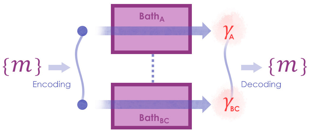
The connection between Communication and Thermodynamics given by Theorem 4 implies that it is impossible for a full thermalization, i.e., for a given thermal state , to transmit any amount of classical information. This is consistent with our physical intuition since a full thermalization means a complete destroy of the input information, leaving no freedom for the output. However, this impossibility can be flipped with the help of pre-shared randomness, which is a pure classical resource. More precisely, when local baths in a bipartite setting are allowed to be correlated through shared randomness, it is possible for locally performed full thermalizations to globally transmit classical information.
To make the statement precise, let us recall the following notions from Ref. Hsieh2020-2 . A bipartite channel on is called a local thermalization to a given pair of thermal states if (1) there exist an ancillary system , unitary channels , and a thermal state separable in bipartition such that and (2) and for all . As mentioned in Ref. Hsieh2020-2 , local thermalization is local in two senses: It is a local operation plus pre-shared randomness channel, and it is locally equivalent to a full thermalization process. The main message from Ref. Hsieh2020-2 is that entanglement preserving local thermalization exists; that is, for every non-pure full-rank , there exists a local thermalization such that is entangled for some . It turns out that such channels can also transmit classical information. To state the result, consider a tripartite system with local dimension , respectively. We focus on the bipartition ; namely, the subsystem can be understood as an ancillary system possessed by the agent in . Let be the thermal state of the subsystem with temperature and Hamiltonian . Following Ref. Hsieh2020-2 , we assume each is non-degenerate and finite-energy. Then, Combining Ref. Hsieh2020-2 and results in Sec. V, in Appendix I we prove that locally performed thermalization is able to transmit classical information with the help of pre-shared randomness [let and ; see also Fig. 1]:
Theorem 6.
When and , there exists an entanglement preserving local thermalization to , denoted by , such that
| (15) |
for every .
Under the global dynamics given by Theorem 6, although the local agents will observe a full thermalization process, transmitting classical information is still possible via the joint bipartite dynamics. This is because classical information can be locally encoded in the global quantum correlation. Note that the amount of transmissible classical information largely depends on local temperatures: When the local systems are too cold (which corresponds to the limit ), a low temperature will force the local thermal state be closed to a pure state (here we assume no energy degeneracy), resulting in no possibility to maintain global correlation. Also note that although is locally identical to a full thermalization process, its global behavior is far from a thermalization. This gap between local and global dynamics leads to the possibility for a classical communication through local thermalizations when shared randomness is accessed to. Notably, this illustrate that, although being a classical resource, shared randomness provides advantages to maintain quantum correlation and assist classical communication through thermalization processes.
VII Conclusion
We study classical communication scenarios with free operations of a given resource as the information processor. The one-shot classical capacity is upper bounded by resource preservability Hsieh2020-1 plus a term of resourceless contribution. This upper bound provides an alternative interpretation of resource preservability. Furthermore, when asymmetry is the resource, a lower bound can also be obtained.
As an application, we use our result to bridge two seemingly different concepts: Under the thermalization model given by Ref. Sparaciari2019 , for every Gibbs-preserving coherence non-generating channel, its smallest channel bath size (i.e., a bath size needed to thermalize all outputs of a given channel) plus its coherence preservability will upper bound its one-shot classical capacity. Thus, under this setting, transmitting bits of classical information through a coherence-annihilating channel requires the channel bath size to be at least , up to some small terms. This reveals an implicit thermodynamic cost of transmitting classical information, providing a dynamical analogue of the Landauer’s principle Landauer1961 and illustrating how a dynamical resource theory allows applications to connect different dynamical phenomena.
We further apply our approach to study channel’s simultaneous maintainability of orthogonality and maximal entanglements. Formulating the question into a communication form, a capacity-like measure can be introduced and upper bounded by resource preservability.
Finally, applying the thermalization channel introduced in Ref. Hsieh2020-2 to a bipartite setting, we show that classically correlated local baths allow a decent amount of one-shot classical capacity even when both local systems are completely thermalized. Hence, classical information processing and thermalization processes can coexist, which only requires shared randomness as a resource. This result also means that when a many-body system is in contact with a global bath having classical correlations within, it is possible to maintain classical information even after it has been thermalized locally. Share randomness as a resource is enough to guarantee that certain amounts of classical information can be extracted after local thermalizations, provided that local temperatures are not too low.
Several open questions remain. First, currently all the results related to resource preservability (e.g., Ref. Hsieh2020-1 ) are focusing on the one-shot regime, and a future direction is to understand its asymptotic behavior. Furthermore, whether one can derive a lower bound similar to Theorem 3 in terms of resource preservability and even extend the result to other state resources are still unknown. These questions could be difficult and largely depend on the choice of resources, since, e.g., the lower bound on the capacity used in Ref. Korzekwa2019 is given by the information spectrum relative entropy, which is not a contractive generalized distance measure Leditzky-PhD and hence cannot induce legal resource preservability monotone. Also, whether one can obtain any result similar to Theorem 5 in the context of coherence is still unknown. Finally, as a direct consequence of Theorem 4, we have the following conjecture: Transmitting bits of classical information through a Gibbs-preserving coherence-annihilating channel requires the corresponding channel bath size to be at least . This conjecture could largely depend on the underlying communication setup and the thermalization model.
We hope the physical messages provided by this work can offer alternative interpretations in the interplay of dynamical resource theory, classical communication, thermodynamics, and different forms of inseparability.
Acknowledgements
We thank Antonio Acín, Stefan Buml, Dario De Santis, Yeong-Cherng Liang, Matteo Lostaglio, Mohammad Mehboudi, Gabriel Senno, and Ryuji Takagi for fruitful discussions and comments. This project is part of the ICFOstepstone - PhD Programme for Early-Stage Researchers in Photonics, funded by the Marie Skłodowska-Curie Co-funding of regional, national and international programmes (GA665884) of the European Commission, as well as by the ‘Severo Ochoa 2016-2019’ program at ICFO (SEV-2015-0522), funded by the Spanish Ministry of Economy, Industry, and Competitiveness (MINECO). We also acknowledge support from the Spanish MINECO (Severo Ochoa SEV-2015-0522), Fundació Cellex and Mir-Puig, Generalitat de Catalunya (SGR1381 and CERCA Programme).
Appendix A Being Realizable Without Consuming Resource and Being Resource Non-Generating Are Not Equivalent
In order to study channels constrained by a given static resource , it is straightforward to expect these channels to be free from . In this work, we depict this by requiring those channels to be “unable to generate .” This coincides with the notion of being non-generating RT-RMP , and hence being free operations of . Meanwhile, there is another possible approach, which is requiring those channels to be “realizable without consuming .” It turns out that this latter option is less generic and accessible compared with the former. This Appendix aims to briefly make this difference clear.
In a given resource theory, either static, dynamical, or a more general one, requiring an operation to be free from the resource sometimes includes two seemingly equivalent concepts implicitly; namely, being realizable without consuming the resource, and being unable to generate the resource. While these two concepts match for some settings, in general they are not equivalent. For instance, the resource theories of entanglement equipped with local operation and classical communication (LOCC) channels or local operation plus pre-shared randomness (LOSR) channels allow this property, and so does the resource theory of nonlocality with LOSR channels. This is because LOCC (so do LOSR) channels can be realized without touching and using any entangled state. Nevertheless, the resource theory of athermality demonstrates a counterexample. In this case, the only free state is the state in thermal equilibrium, i.e., the thermal state . Physically, it is impossible to realize any non-trivial channel only within thermal equilibrium (the only realizable one is the state preparation channel of , since one can artificially switch with the input and discard the original system). On the other hand, a commonly used free operation is the thermal operation, which takes the form , where conserves the total energy (i.e., it commutes with the total Hamiltonian). One can see that any non-trivial thermal operation (which is athermality non-generating) needs a non-trivial unitary , and hence includes effects out of thermal equilibrium; i.e., it is not realizable without consuming athermality.
Apart from resource theories of states, there are also instances in dynamical resource theories illustrating this difference. In the resource theory for non-signaling assisted classical communication Takagi2019-3 , the free quantities are state preparation channels, and it is impossible to output channels useful for classical communication if one only uses state preparation channels to implement free super-channels. Similarly, in the theory of resource preservability Hsieh2020-1 , it is again impossible to output resourceful channels when one only uses resource annihilating channels to implement free super-channels.
If one upgrades the discussion to general and abstract considerations, it can be tough to access the detailed physical structures of operations. Consequently, the best one can do is to analyze an operation by comparing its inputs and outputs. This is also the only way to check whether an operation is free from the given resource. Hence, “zero ability to generate the resource” ends up to be the most feasible and well-defined way to depict “begin free” in the most general extend when further structures and contexts are not available. Being realizable without consuming the resource is an additional property that can be satisfied in certain cases, but this notion could be generally ill-defined.
Note that this is also why in a general, model-independent level, the definition of being resource non-generating only requires no generation of the resource for free inputs: Before introducing free operations, we cannot compare and order different resourceful states, and the only existing concept before defining free operations is “whether the quantity is resourceful or not.” This gives us the most extensive range to clarify the notion of “being free from the resource.” It also briefly summarizes the features of central ingredients in a resource theory: Free states give us detection, free operations give us comparison, and monotones give us quantification.
Due to the above discussion, in this work, we depict a channel as constrained by a resource if it is a free operation.
Appendix B Assumptions on State Resource Theories for Resource Preservability Theories
To have a general study that is also analytically feasible, we need to impose certain assumptions on the state resource theories considered in this work. Let be a given state resource theory. Then we consider
-
1.
Identity channel and partial trace are both free operations; namely, they are both in .
-
2.
Free operations are closed under tensor products, convex sums, and compositions: For every and , we have , , and .
-
3.
For every system there exists a state such that is a free operation.
Assumptions 1 and 2 are always assumed in this work in order to capture the necessary properties of a monotone, and we leave Assumption 3 optional. This is slightly different from Ref. Hsieh2020-1 , and our motivation is to relax the assumptions made by Ref. Hsieh2020-1 to achieve a general consideration admitting more applicable cases. We briefly explain each assumptions. Assumption 1 follows from our conceptual expectation; that is, “doing nothing” and “ignoring part of the system” are both unable to generate . Assumption 2 implies that if two channels are unable to generate , then neither can their simultaneous application (tensor product), classical mixture (convex sum), and sequential application (composition). Finally, Assumption 3 ensures that there always exists a “free extension,” which automatically implies the state is free an hence (to see this, consider and use Assumptions 1 and 2). Note that Assumption 3 is only imposed on systems with proper system sizes. For example, in the resource theory of entanglement, steering, and nonlocality, must be bipartite (and we always assume equal local dimension); in the resource theory of athermality, can only have dimension with some positive integer , where is the dimension of the given thermal state.
Many known resource theories share these assumptions. For instance, Assumptions 1, 2, and 3 are satisfied by the sets of LOCC channels, LOSR channels, Gibbs-preserving maps, and -covariant channels (in multipartite cases, we consider the group ). Note that Assumption 3 holds since for every system with dimension the mapping is an LOSR and -covariant channel. The case of Gibbs-preserving maps (with the thermal state ) follows from the fact that is Gibbs-preserving for all . This implies the validity of Assumptions 1, 2, and 3 in the following state resource theories, which covers most of the cases studied in this work: (i) entanglement and free entanglement Horodecki1998 equipped with LOCC or LOSR channels, (ii) nonlocality, steering, multi-copy nonlocality, and multi-copy steering equipped with LOSR channels (see Appendix B.2 for a discussion), (iii) -asymmetry equipped with -covariant channels, and (iv) athermality equipped with Gibbs-preserving maps.
It turns out that, by using Assumptions 1, 2, and 3, we can prove a generalized version of Theorem 2 in Ref. Hsieh2020-1 , which is summarized as follows:
Theorem B.1.
Hsieh2020-1 is a state resource theory satisfying Assumptions 1 and 2. is a contractive generalized distance measure of states. Then satisfies
-
1.
and if .
-
2.
for every channel and free super-channel .
If Assumption 3 holds, then we have
| (16) |
for every , and the equality holds if .
Proof.
Apart from Eq. (49) in Ref. Hsieh2020-1 , the proof is the same with the one of Theorem 2 in Ref. Hsieh2020-1 (see Eqs. (48) and (50) in Ref. Hsieh2020-1 ). Note that Eq. (48) in Ref. Hsieh2020-1 works for every channel, which explains the validity of statement 2 in this theorem. It remains to show Eq. (7) in Ref. Hsieh2020-1 , which can be seen by the following alternative proof:
| (17) |
The second line follows from the data-processing inequality and the fact that has a well-defined marginal in Acknowledgement . In the third line, forms a sub-optimal range of the maximization, where is the state guaranteed by Assumption 3 that allows the map to be a free operation of . Together with Assumptions 1 and 2, we learn that is a resource annihilating channel, which forms a sub-optimal range of the minimization and implies the fourth line. Hence, Assumptions 1, 2, and 3 are enough to ensure the correcteness of Theorem 2 in Ref. Hsieh2020-1 . ∎
Theorem B.1 generalizes Theorem 2 in Ref. Hsieh2020-1 by relaxing the assumptions of absolutely free states (i.e., the assumptions (R1) and (R3) in Ref. Hsieh2020-1 ) into Assumption 3. Furthermore, there is no need to assume the convexity of . Another remark is that non-increasing under free super-channel actually works for every channel, including channels that are not free operations. This is a useful observation when one needs to consider the smooth version of -preservability, e.g., in the next sub-section.
B.1 Properties of
We remark that , which can be interpreted as the smooth version of , still possesses the expected properties that a monotone should have. First, if , then we have . The non-increasing property under free super-channels can be summarized in the following lemma:
Lemma B.2.
For every channel , , and , we have
| (18) |
Proof.
We note the following estimate first:
| (19) |
The first inequality follows from the data processing inequality, or equivalently, the contractivity of the trace norm; the second ineuqality follows from the definition of the diamond norm. Recall that will take the form . We conclude that
| (20) |
where the second line follows from data-processing inequality, the fourth line is because induces a sub-optimal range of the maximization in the definition of diamond norm. In the last line we use Eq. (B.1). Now, direct computation shows
| (21) |
From Eq. (B.1) we learn that all channels satisfying form a subset of all channels satisfying . This explains the second line. The third line follows from Theorem B.1 (note that could be outside , but it is still a channel). In the fourth line, we have the set of all channels of the form be a subset of the set of all channels. This shows the desired claim. ∎
B.2 LOSR Channels as Free Operations of Nonlocality, Steering, Multi-Copy Nonlocality, and Multi-Copy Steering
Appendix A.1 in Ref. Hsieh2020-1 explains that LOSR channels can be free operations of nonlocality. Here, we briefly show that LOSR channels can also be free operations of three other different forms of inseparabilities: Steering Wiseman2007 ; Jones2007 ; steering-review ; RMP-steering , multi-copy nonlocality Palazuelos2012 ; Cavalcanti2013 , and multi-copy steering Hsieh2016 ; Quintino2016 . Formally, a LOSR channel in a given bipartite system is given by the following form:
| (22) |
where the integration is taken over the parameter . Physically, it is a convex mixture of local dynamics. Now, in the given bipartite system , a state is unsteerable from to Wiseman2007 ; Jones2007 ; steering-review ; RMP-steering , or simply unsteerable, if for every local POVMs in and in , one can write
| (23) |
for some variable in a set , some probability distributions , and some local states in . In other words, a state is unsteerable if every outcome of local measurements in is indistinguishable from the outputs of pre-shared randomness combined with local quantum theory in . Such models are called local hidden state models Wiseman2007 ; Jones2007 ; steering-review ; RMP-steering , as depicted by . States that are not unsteerable are said to be steerable.
To see why LOSR channels can be free operations for steering, consider an LOSR channel and the following computation
| (24) |
where and again form local POVMs since are completely-positive unital maps. Hence, when is unsteerable, it means, for every , we can write as Eq. (23). This means the output of Eq. (B.2) is again described by Eq. (23).
With the notions of nonlocality and steering, we say a state is multi-copy nonlocal Palazuelos2012 (and, similarly, multi-copy steerable Hsieh2016 ; Quintino2016 ) if is nonlocal ( steerable) for some positive integer . One can see that LOSR channels again act as free operations for these two resources. To see this, it suffices to observe that if is an LOSR channel in a given bipartition, then will again be an LOSR channel in the same bipartition. More precisely, consider an LOSR channel in bipartition. Suppose is multi-copy local ( unsteerable) in this bipartition; namely, is local ( unsteerable) for all . Then, for all , must be local ( unsteerable) since is local ( unsteerable) and is again an LOSR channel in the bipartition. This shows that LOSR channels can be free operations of multi-copy nonlocality and multi-copy steering.
Appendix C Proofs of Theorem 1 and Corollary 2
First, we note the following lemma similar to Fact E.2 in Ref. Hsieh2020-1 . This will enable us to obtain an equivalent representation of defined in Eq. (4). In what follows, the maximization is taken over all ancillary systems , absolutely resource annihilating channels , and joint input states . Note that the maximization includes the trivial ancillary system (i.e., the one with dimension 1), which means it also covers the case when there is no ancillary system.
Lemma C.1.
Given two channels and , then we have
| (25) |
Proof.
Let , where is a specific combination of , , and . Then the left-hand-side is , and the right-hand-side is . The inequality “” follows since for all . To show the opposite, consider an arbitrary positive integer . Then there exist and such that
| (26) | |||
| (27) |
This means for all , which further implies . We conclude that
| (28) |
and the desired claim follows by considering all possible . ∎
Fact C.2.
is a positive map .
Proof.
Suppose the opposite was correct. Then there exists an ancillary system , an absolutely resource annihilating channel , two states , such that . However, we have due to Eq. (C). This leads to a contradiction when . ∎
Finally, we note the following alternative form of Eq. (4):
| (30) |
C.1 Proof of Theorem 1
Proof.
Consider a channel satisfying . For a given error , recall that , which is by definition non-empty. Then for every , Fact C.2 implies the existence of a positive map such that
| (31) | |||
| (32) |
Note that the positivity of actually follows from Eq. (31) and the fact that one is allowed to consider the trivial ancillary system, i.e., the case when there is no ancillary system. Now, with a given -code , we have [recall the definition from Eq. (2)]:
| (33) |
where the facts that and for all imply the third line, and the maximization is taken over every and -code . Since this is true for every , we conclude the following with Eq. (6):
| (34) |
Now we use the estimate Takagi2019-3 , where is the diamond norm. This can be seen by the following computation
| (35) |
which follows from the estimate Takagi2019-3 for arbitrary channels . Gathering the above ingredients, we conclude that for every channel satisfying and -code achieving , we have
| (36) |
In other words, for every given satisfying we have
| (37) |
and the result follows. ∎
C.2 Remark
Note that in some cases Eq. (7) can be simplified. For instance, when the free states are isotropic states Horodecki1999-2 (i.e., is asymmetry of the group ), then footnote:IsotropicStates . When , Theorem 1 implies , and the additional degrees of freedom of -asymmetry allow performance better than isotropic states. Another example is when is athermality, which implies Corollary 2 that will be proved in the following sub-section.
C.3 Proof of Corollary 2
Proof.
First, from Eq. (80) in Ref. Hsieh2020-1 we learn that . This means that and hence
| (38) |
and the result follows. ∎
Appendix D Proof of Theorem 3
Proof.
We follow the proof of Theorem 2 in Ref. Korzekwa2019 . First, a -twirling channel, which is an operation used to symmetrize all input states with respect to a unitary group , is defined by
| (39) |
When the group is infinite, one can replace the summation by integration equipped with the Haar measure: We focus on the finite case to illustrate the proof.
With a given state and a given codebook (that is, a mapping, , from the classical information to the set ) Korzekwa2019 , consider the encoding
| (40) |
To construct the decoding, consider the following elements of POVM (which is a pretty good measurement scheme):
| (41) |
where . Note that for a positive semi-definite operator , the notation is the inverse of restricted to the support of Beigi2014 . This means will be the projection onto the support of , and we have in general. Hence, is not a POVM in general, since will be the projection onto the support of . Recently, Korzekwa et al. (see Eqs. (44), (45) and (51) in Ref. Korzekwa2019 ) show that for we have
| (42) |
where indicates the average over randomly chosen codebook (following Ref. Korzekwa2019 , each is independently and uniformly at random encoded into the integer , which means can be interpreted as independent and identically distributed random variables with uniform distribution). For a -covariant channel , consider the -code given by , where for and . Note that is the projection onto the support of , which means . Then we have
| (43) |
Since is non-negative, the second line follows. The third line is because is -covariant and , so we have . The last line is a direct application of Eq. (42) by replacing the role of by . This means when , there must exist an -code with some and achieving . Let . Because no -code can achieve success probability , we must have
| (44) |
Following Ref. Korzekwa2019 , we set . Since for all positive integer , we conclude that
| (45) |
where the first line is a direct consequence of Eq. (44), and the second line is because is an -covariant channel that can only output symmetric states. ∎
Appendix E Collision Model for Thermalization
Following Ref. Sparaciari2019 , consider a finite dimensional system S with Hamiltonian and a bath , which is assumed to be copies of the system , and each copy has Hamiltonian . Labeling the bath as , this means . The collision model introduced in Ref. Sparaciari2019 used to depict thermalization processes is given by
| (46) |
where is the global state on at time , represents an energy-preserving unitary on ; i.e., , and is the rate for to occur (see also Eqs. (A2) and (A3) in Appendix A of Ref. Sparaciari2019 ). Roughly speaking, each models an elastic collision between certain subsystems of . We refer the reader to Ref. Sparaciari2019 for the details of the model and its physical reasoning. In this work, we use the notation to denote the set of channels on such that, for every in , can be realized by Eq. (46) at a time point [i.e., ; note that we also allow ] with . See also Ref. Hsieh2020-1 for its connection with resource preservability.
Appendix F Proof of Theorem 4
Theorem 4 is a consequence of the combination of Theorem 1 and Theorem 4 in Ref. Hsieh2020-1 , which is formally stated as follows (here we implicitly assume the system Hamiltonian is the one realizing the thermal state with some temperature):
Theorem F.1.
Hsieh2020-1 Given a Gibbs-preserving channel , , and a full-rank thermal state . If is coherence-annihilating and the system Hamiltonian satisfies the energy subspace condition, then we have
| (47) |
where is the smallest eigenvalue of .
We remark that being coherence-annihilating is required by the proof given in Ref. Sparaciari2019 (specifically, it is crucial for the proof of Lemma 17 in Appendix C of Ref. Sparaciari2019 ), which explains the assumption made in Theorem 4. Combining Corollary 2 (and hence Theorem 1) and Theorem F.1, we are now in the position to prove Theorem 4:
Appendix G Proof of Theorem 5
Before the proof, let us recall a crucial tool called fully entangled fraction (FEF) Horodecki1999-2 ; Albeverio2002 . For a bipartite state with equal local dimension , its FEF is defined by
| (50) |
which maximizes over all maximally entangled states with local dimension . FEF is well-known for characterizing different forms of inseparability Horodecki1999-2 ; Albeverio2002 ; Zhao2010 ; Cavalcanti2013 ; Bell-RMP ; Quintino2016 ; Hsieh2016 ; Hsieh2018E ; Ent-RMP ; Liang2019 ; Hsieh2020-2 . For instance, implies is free entangled Ent-RMP ; Horodecki1999-1 , useful for teleporation Horodecki1999-2 , multi-copy nonlocal Palazuelos2012 ; Cavalcanti2013 , and multi-copy steerable Hsieh2016 ; Quintino2016 (see also Appendix B.2).
Following the proof of Theorem 1, we will prove a lemma and have the main theorem as a corollary. Given a state resource , recall from Sec. II that is the set of free operations of -preservability given by Hsieh2020-1 , where are free operations and is an absolutely resource annihilating channel. Since now, we will always assume that for every and , the input and output systems of are both bipartite with finite equal local dimension. Also, we will use the notation to denote the set of free states of in bipartite systems with equal local dimension .
Lemma G.1.
Given satisfying . For and , if achieves , then we have
| (51) |
where
| (52) |
and is the local dimension of the output bipartite system of .
Proof.
For every positive integer and every such that , Eq. (30) implies the existence of a value and a -annihilating channel such that (i) , and (ii) is a positive map for every ancillary system and , where . Write with and . This means for every positive integer we have (note that ’s are all staying in the output space of , which is a bipartite system with equal local dimension ):
| (53) |
The second line is because is a positive map. The third line is because , and the fact that the output system is a bipartite system with equal local dimension . From here we conclude that
| (54) |
As a direct observation on Lemma G.1, once has an explicit dependency on , one could conclude an upper bound on . This is the case for various resources, and this fact allows us to prove Theorem 5 as follows.
Proof.
In the first case, consider athermality with the thermal state , which is in a bipartite system with equal local dimension. Then it suffices to notice that in this case Eq. (G) becomes
| (56) |
This means we have for all , and the desired bound follows.
Now we recall that a bipartite state with equal finite local dimension is free entangled Ent-RMP ; Horodecki1998 , multi-copy nonlocal Palazuelos2012 ; Cavalcanti2013 , and multi-copy steerable Hsieh2016 ; Quintino2016 if . This means for these resources we have . Given and , Lemma G.1 implies that for every achieving , we have [in what follows we again use to denote the local dimension of the output bipartite system of ]
| (57) |
where the second line is because for any such the output space of contains mutually orthonormal maximally entangled states, which means and hence . From here we conclude that
| (58) |
which is the desired bound by considering all possible and . ∎
Appendix H Implications of Theorem 5
Theorem 5 gives further implications to superdense coding and also connects FEF and resource preservability. We briefly summarize these remarks in this appendix.
H.1 Maintaining Orthogonal Maximal Entanglement and Superdense Coding
Theorem 5 allows an interpretation for superdense coding, and we briefly introduce the setup here to illustrate this. Consider two agents, Alice and Bob, sharing a maximally entangled state with local dimension . First, Alice encodes the classical information in her local system (a qudit) by applying , the unitary operator achieving with a given set of orthogonal maximally entangled states . After this, she sends her qudit to Bob, and both Alice’s and Bob’s qudits undergo a dynamics modeled by a bipartite channel . After receiving Alice’s qudit, Bob decodes the classical information from by a bipartite measurement. We call such task a dimensional superdense coding through . It is the conventional superdesne coding when , where Bob can apply a dimensional Bell measurement to perfectly decode classical data when only one qudit has been sent. In general, different channels have different abilities to admit superdense coding, and is the highest amount of classical information allowed by a dimensional superdense coding through a channel even with all possible assistance structures constrained by , i.e., . In this sense, can be understood as the superdense coding ability of , and Theorem 5 estimates the optimal performance of superdense coding.
H.2 Fully Entangled Fraction and Resource Preservability
It is worth mentioning that the proof of Theorem 5 largely relies on FEF. Once an FEF threshold with an explicit dependency of local dimension exists, a result similar to Theorem 5 can be obtained. For example, from Ref. Hsieh2016 we learn that is (two-way) steerable if . This means when (two-way) steerability and , we have Hence, when (two-way) steerability, we have
| (59) |
It turns out that resource preservability can be related to FEF as follows
Proposition H.1.
Given a resource , then cannot maintain any maximally entangled state with an average error less than if
| (60) |
where is the local dimension of the output bipartite space of .
Proof.
Applying Lemma G.1 with , we learn that there exists no that can achieve if
| (61) |
In other words, cannot maintain any maximally entangled state with an average error lower than when this inequality is satisfied. ∎
Proposition H.1 gives a new way to understand FEF: Once a channel’s resource preservability is not strong enough compared with a threshold induced by FEF, it is impossible to maintain maximal entanglement to the desired level. For examples, suppose is a free operation of free entanglement (or, similarly, multi-copy nonlocality or multi-copy steerability; note that we need to assume Assumptions 1 and 2), then Proposition H.1 implies that cannot maintain any maximally entangled state with an average error lower than if
Appendix I Proof of Theorem 6
To demonstrate the proof, we will first provide a generalized version of the entanglement preserving local thermalization introduced in Ref. Hsieh2020-2 . After that, Theorem 6 can be proved by using it and the capacity-like measure defined in Eq. (13). Before proceeding, we remark that, in this appendix, we will use subscripts to denote the located subsystems for both states and channels; e.g., and are a state and a channel in the system , respectively. Also, following Ref. Hsieh2020-2 , we assume no energy degeneracy for all subsystems, and all thermal states are assumed to be full-rank.
To start with, we recall from Ref. Hsieh2020-2 the following alternative definition of a local thermalization with a given pair of thermal states on the subsystem , respectively [recall from Eq. (22) the definition of local operation and pre-shared randomness (LOSR) channels]:
Definition I.1.
Hsieh2020-2 A bipartite channel on is called a local thermalization to if
-
1.
is a LOSR channel in bipartition.
-
2.
and for all states .
As remarked in Ref. Hsieh2020-2 , a local thermalization is local in the sense that it is a LOSR channel that can locally thermalize all inputs. This definition is equivalent to the one given in the main text, and we refer the reader to Definition 1, Definition 2, and Theorem 2 in Ref. Hsieh2020-2 for the detailed reasoning.
Now, consider a tripartite system with finite local dimensions , respectively. As mentioned in the main text, we will focus on the bipartition , and the subsystem can be treated as an ancillary system possessed by the local agent in . In what follows, is the given thermal state of the subsystem with temperature and Hamiltonian . Suppose is the orthonormal energy eigenbasis of with local dimension . Then we define the following channel, which has a schematic interpretation given in Fig. 2. First, consider a given ordered set of local unitary operators in denoted by where is always assumed to be the maximally mixed state, and other elements are arbitrary. Then, for every , we define
| (62) |
whose components are defined as follows. First, in a bipartite system with finite equal local dimension,
| (63) |
is the -twirling operation Horodecki1999-1 ; Bennett1996 used to symmetrize the local states. To encode classical information into the correlation shared by , we define the following local channel in :
| (64) |
Using operator-sum representation QCI-book , one can check that this is indeed a channel. Finally,
| (65) |
where
| (66) |
is an alternative thermal state for . Let , which is the smallest eigenvalue among . Write , then we have the following result:
Theorem I.2.
For every and , we have
-
1.
is a local thermalization to for all .
-
2.
is an entanglement preserving local thermalization to for all full-rank and .
Proof.
Following Lemma 1 in Ref. Hsieh2020-2 , we conclude that the local output of in and will always be and , respectively. Also, guarantees that both are legal quantum states. This implies that is a legal channel, which is by definition a LOSR channel in the bipartition. Hence, for all , is a local thermalization when is in the desired range. Finally, when and are both full-rank (and hence non-pure), Theorem 1 in Ref. Hsieh2020-2 implies that will be entangled in the bipartition since in the subsystem it is identical to the entanglement preserving local thermalization constructed in Ref. Hsieh2020-2 . This proves the desired claim. ∎
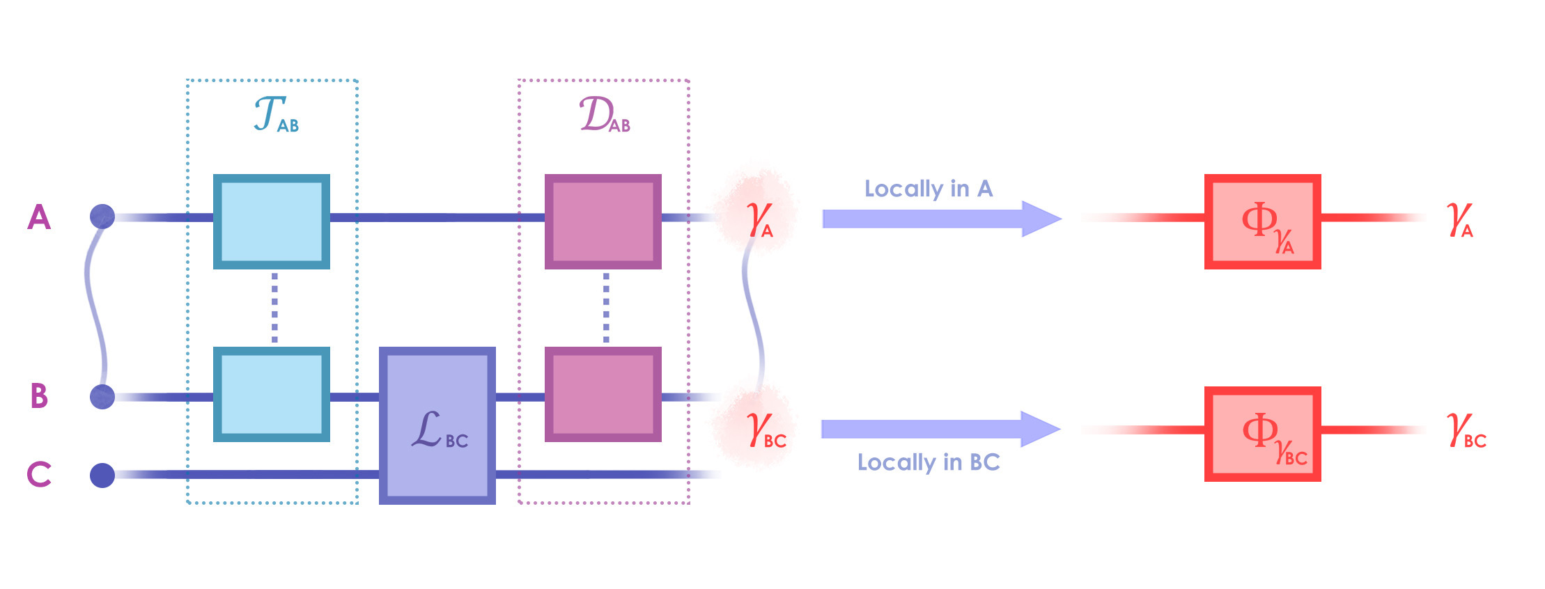
We leave a schematic interpretation in Fig. 2, and now we proceed to prove Theorem 6 by using Theorem I.2:
Proof.
Note that by assuming each subsystem Hamiltonian to be non-degenerate and finite-energy, the corresponding thermal state is non-pure and full-rank if and only if Hsieh2020-2 . Hence, for every , we conclude that is an entanglement preserving local thermalization to according to Theorem I.2. Now we note that the one-shot classical capacity of can be estimated by the ability of to maintain maximally entangled bases (see Sec. V). More precisely, for a given and sets of orthonormal maximally entangled states (in the bipartition) , the corresponding success probability of reads . Being maximally entangled, there exist unitary operators in , , such that , where . Define the set with for all . Now we choose the encoding as
| (67) |
and decoding POVM as
| (68) | |||
| (69) |
Then we have
| (70) |
where the inequality is due to the fact that . This means [see Eq. (13) for the definition of ]
| (71) |
where the optimization is taken over every possible ordered set of unitary operators with . On the other hand, we have
| (72) |
Note that has output system dimension . Hence, when , the success probability is given by This means that if , or, equivalently,
| (73) |
Consequently, by using Eq. (71), we learn that when Eq. (73) holds, there must exists an such that . The result follows. ∎
References
- (1) E. Chitambar and G. Gour, Quantum resource theories, Rev. Mod. Phys. 91, 025001 (2019).
- (2) R, Horodecki, P, Horodecki, M, Horodecki, and K, Horodecki, Quantum entanglement, Rev. Mod. Phys. 81, 865 (2009).
- (3) M. A. Nielsen and I. L. Chuang, Quantum Computation and Quantum Information, (Cambridge University Press, Cambridge, UK, 2000).
- (4) L. Wang and R. Renner, One-shot classical-quantum capacity and hypothesis testing, Phys. Rev. Lett. 108, 200501 (2012).
- (5) N. Datta, M. Mosonyi, M.-H. Hsieh, and F. G. S. L. Brando, A smooth entropy approach to quantum hypothesis testing and the classical capacity of quantum channels, IEEE Trans. Inf. Theory 59, 8014 (2013).
- (6) V. Vedral, M. B. Plenio, M. A. Rippin, and P. L. Knight, Quantifying entanglement, Phys. Rev. Lett. 78, 2275 (1997).
- (7) G. Vidal and R. F. Werner, Computable measure of entanglement, Phys. Rev. A 65, 032314 (2002).
- (8) A. Streltsov, G. Adesso, and M. B. Plenio, Colloquium: Quantum coherence as a resource, Rev. Mod. Phys. 89, 041003 (2017).
- (9) T. Baumgratz, M. Cramer, and M. B. Plenio, Quantifying coherence, Phys. Rev. Lett. 113, 140401 (2014).
- (10) J. S. Bell, On the Einstein Podolsky Rosen paradox, Physics Physique Fizika 1, 195 (1964).
- (11) N. Brunner, D. Cavalcanti, S. Pironio, V. Scarani, and S. Wehner, Bell nonlocality, Rev. Mod. Phys. 86, 419 (2014).
- (12) E. Wolfe, D. Schmid, A. B. Sainz, R. Kunjwal, and R. W. Spekkens, Quantifying Bell: The resource theory of nonclassicality of common-cause boxes, Quantum 4, 280 (2020).
- (13) H. M. Wiseman, S. J. Jones, and A. C. Doherty, Steering, entanglement, nonlocality, and the Einstein-Podolsky-Rosen paradox, Phys. Rev. Lett. 98, 140402 (2007).
- (14) S. J. Jones, H. M. Wiseman, and A. C. Doherty, Entanglement, Einstein-Podolsky-Rosen correlations, Bell nonlocality, and steering, Phys. Rev. A 76, 052116 (2007).
- (15) D. Cavalcanti and P. Skrzypczyk, Quantum steering: A review with focus on semidefinite programming, Rep. Prog. Phys. 80, 024001 (2017).
- (16) R. Uola, A. C. S. Costa, H. C. Nguyen, and O. Ghne, Quantum steering, Rev. Mod. Phys. 92, 015001 (2020).
- (17) P. Skrzypczyk, M. Navascués, and D. Cavalcanti, Quantifying Einstein-Podolsky-Rosen steering, Phys. Rev. Lett. 112, 180404 (2014).
- (18) M. Piani and J. Watrous, Necessary and sufficient quantum information characterization of Einstein-Podolsky-Rosen steering, Phys. Rev. Lett. 114, 060404 (2015).
- (19) R. Gallego and L. Aolita, Resource theory of steering, Phys. Rev. X 5, 041008 (2015).
- (20) G. Gour and R. W. Spekkens, The resource theory of quantum reference frames: Manipulations and monotones, New J. Phys. 10, 033023 (2008).
- (21) I. Marvian and R. W. Spekkens, How to quantify coherence: Distinguishing speakable and unspeakable notions, Phys. Rev. A 94, 052324 (2016).
- (22) R. Takagi, Skew informations from an operational view via resource theory of asymmetry, Sci. Rep. 9, 14562 (2019).
- (23) F. G. S. L. Brando, M. Horodecki, J. Oppenheim, J. M. Renes, and R. W. Spekkens, Resource theory of quantum states out of thermal equilibrium, Phys. Rev. Lett. 111, 250404 (2013).
- (24) M. Horodecki and J. Oppenheim, Fundamental limitations for quantum and nanoscale thermodynamics, Nat. Commun. 4, 2059 (2013).
- (25) F. G. S. L. Brando, M. Horodecki, N. Ng, J. Oppenheim, and S. Wehner, The second laws of quantum thermodynamics, Proc. Natl. Acad. Sci. U.S.A. 112, 3275 (2015).
- (26) M. Lostaglio, An introductory review of the resource theory approach to thermodynamics, Rep. Prog. Phys. 82, 114001 (2019).
- (27) V. Narasimhachar, S. Assad, F. C. Binder, J. Thompson, B. Yadin, and M. Gu, Thermodynamic resources in continuous-variable quantum systems, arXiv:1909.07364.
- (28) A. Serafini, M. Lostaglio, S. Longden, U. Shackerley-Bennett, C.-Y. Hsieh, and G. Adesso, Gaussian thermal operations and the limits of algorithmic cooling, Phys. Rev. Lett. 124, 010602 (2020).
- (29) M. Horodecki and J. Oppenheim, (Quantumness in the context of) resource theories, Int. J. Mod. Phys. B 27, 1345019 (2013).
- (30) F. G. S. L. Brando and G. Gour, Reversible framework for quantum resource theories, Phys. Rev. Lett. 115, 070503 (2015).
- (31) L. del Rio, L. Kraemer, and R. Renner, Resource theories of knowledge, arXiv:1511.08818.
- (32) B. Coecke, T. Fritz, and R. W. Spekkens, A mathematical theory of resources, Inf. Comput. 250, 59 (2016).
- (33) G. Gour, Quantum resource theories in the single-shot regime, Phys. Rev. A 95, 062314 (2017).
- (34) Z.-W. Liu, X. Hu, and S. Lloyd, Resource destroying maps, Phys. Rev. Lett. 118, 060502 (2017).
- (35) A. Anshu, M.-H. Hsieh, and R. Jain, Quantifying resources in general resource theory with catalysts, Phys. Rev. Lett. 121, 190504 (2018).
- (36) L. Lami, B. Regula, X. Wang, R. Nichols, A. Winter, and G. Adesso, Gaussian quantum resource theories, Phys. Rev. A 98, 022335 (2018).
- (37) B. Regula, Convex geometry of quantum resource quantification, J. Phys. A: Math. Theor. 51, 045303 (2018).
- (38) Z.-W. Liu, K. Bu, and R. Takagi, One-shot operational quantum resource theory, Phys. Rev. Lett. 123, 020401 (2019).
- (39) K. Fang and Z.-W. Liu, No-go theorems for quantum resource purification, Phys. Rev. Lett. 125, 060405 (2020).
- (40) R. Takagi and B. Regula, General resource theories in quantum mechanics and beyond: Operational characterization via discrimination tasks, Phys. Rev. X 9, 031053 (2019).
- (41) R. Takagi, B. Regula, K. Bu, Z.-W. Liu, and G. Adesso, Operational advantage of quantum resources in subchannel discrimination, Phys. Rev. Lett. 122, 140402 (2019).
- (42) L. Li, K. Bu and Z.-W. Liu, Quantifying the resource content of quantum channels: An operational approach, Phys. Rev. A 101, 022335 (2020).
- (43) K. Korzekwa, Z. Puchała, M. Tomamichel, and K. yczkowski, Encoding classical information into quantum resources, arXiv:1911.12373.
- (44) Channels, or quantum channels, also known as completely-positive trace-preserving maps QCI-book ), are general mathematical forms used to depict physical processes and dynamics.
- (45) J.-H. Hsieh, S.-H. Chen, and C.-M. Li, Quantifying quantum-mechanical processes, Scientific Reports 7, 13588 (2017).
- (46) C.-C. Kuo, S.-H. Chen, W.-T. Lee, H.-M. Chen, H. Lu, and C.-M. Li, Quantum process capability, Scientific Reports 9, 20316 (2019).
- (47) K. B. Dana, M. G. Díaz, M. Mejatty, and A. Winter, Resource theory of coherence: Beyond states, Phys. Rev. A 95, 062327 (2017).
- (48) S. Pirandola, R. Laurenza, C. Ottaviani, and L. Banchi, Fundamental limits of repeaterless quantum communications, Nat. Commun. 8, 15043 (2017).
- (49) M. G. Díaz, K. Fang, X. Wang, M. Rosati, M. Skotiniotis, J. Calsamiglia, and A. Winter, Using and reusing coherence to realize quantum processes, Quantum 2, 100 (2018).
- (50) D. Rosset, F. Buscemi, and Y.-C. Liang, A resource theory of quantum memories and their faithful verification with minimal assumptions, Phys. Rev. X 8, 021033 (2018).
- (51) M. M. Wilde, Entanglement cost and quantum channel simulation, Phys. Rev. A 98, 042338 (2018).
- (52) Q. Zhuang, P. W. Shor, and J. H. Shapiro, Resource theory of non-Gaussian operations, Phys. Rev. A 97, 052317 (2018).
- (53) S. Buml, S. Das, X. Wang, and M. M. Wilde, Resource theory of entanglement for bipartite quantum channels, arXiv:1907.04181.
- (54) J. R. Seddon and E. Campbell, Quantifying magic for multi-qubit operations, Proc. R. Soc. A 475, 20190251 (2019).
- (55) Z.-W. Liu and A. Winter, Resource theories of quantum channels and the universal role of resource erasure, arXiv:1904.04201.
- (56) Y. Liu and X. Yuan, Operational resource theory of quantum channels, Phys. Rev. Research 2, 012035(R) (2020).
- (57) G. Gour, Comparison of quantum channels by superchannels, IEEE Trans. Inf. Theory 65, 5880 (2019).
- (58) G. Gour and A. Winter, How to quantify a dynamical resource? Phys. Rev. Lett. 123, 150401 (2019).
- (59) G. Gour and C. M. Scandolo, The entanglement of a bipartite channel, arXiv:1907.02552.
- (60) R. Takagi, K. Wang, M. Hayashi, Application of the resource theory of channels to communication scenarios, Phys. Rev. Lett. 124, 120502 (2020).
- (61) T. Theurer, D. Egloff, L. Zhang, and M. B. Plenio, Quantifying operations with an application to coherence, Phys. Rev. Lett. 122, 190405 (2019).
- (62) X. Wang and M. M. Wilde, Resource theory of asymmetric distinguishability for quantum channels, Phys. Rev. Research 1, 033169 (2019).
- (63) G. D. Berk, A. J. P. Garner, B. Yadin, K. Modi, and F. A. Pollock, Resource theories of multi-time processes: A window into quantum non-Markovianity, arXiv:1907.07003.
- (64) G. Saxena, E. Chitambar,and G. Gour, Dynamical resource theory of quantum coherence, Phys. Rev. Research 2, 023298 (2020).
- (65) Y. Zhang, R. A. Bravo, V. O. Lorenz, and E. Chitambar, Channel activation of CHSH nonlocality, New J Phys. 22, 043003 (2020).
- (66) C.-Y. Hsieh, Resource preservability, Quantum 4, 244 (2020).
- (67) H. Kristjánsson, G. Chiribella, S. Salek, D. Ebler, and M. Wilson, Resource theories of communication, New J. Phys. 22, 073014 (2020).
- (68) C. Sparaciari, M. Goihl, P. Boes, J. Eisert, and N. Ng, Bounding the resources for thermalizing many-body localized systems, arXiv:1912.04920.
- (69) R. Landauer, Irreversibility and Heat Generation in the Computing Process, IBM J. Res. Develop., 5, 183 (1961).
- (70) To clarify different notions, note that resource annihilating channels introduced in Ref. Hsieh2020-1 is different from resource destroying maps Liu2017 , where the latter keep free states invariant and map resourceful states to some free states. For instance, a state preparation channel preparing a fixed free state is a legal resource annihilating channel, while it is not a resource destroying map. As another remark, when the resource is entanglement, the notion of resource annihilating channel coincides with entanglement-annihilating channel Moravcikova2010 , which is different from entanglement-breaking channel Horodecki2003 .
- (71) C. Palazuelos, Superactivation of quantum nonlocality, Phys. Rev. Lett. 109, 190401 (2012).
- (72) D. Cavalcanti, A. Acin, N. Brunner, and T. Vertesi, All quantum states useful for teleportation are nonlocal resources, Phys. Rev. A 87, 042104 (2013).
- (73) C.-Y. Hsieh, Y.-C. Liang, and R.-K. Lee, Quantum steerability: Characterization, quantification, superactivation and unbounded amplification, Phys. Rev. A 94, 062120 (2016).
- (74) M. T. Quintino, M. Huber, and N. Brunner, Superactivation of quantum steering, Phys. Rev. A 94, 062123 (2016).
- (75) G. Chiribella, G. M. D’Ariano, and P. Perinotti, Transforming quantum operations: quantum supermaps, EPL (Europhysics Letters) 83, 30004 (2008).
- (76) G. Chiribella, G. M. D’Ariano, and P. Perinotti, Quantum circuit architecture, Phys. Rev. Lett. 101, 060401 (2008).
- (77) N. Datta, Min- and max-relative entropies and a new entanglement monotone, IEEE Trans. Inf. Theory 55, 2816 (2009).
- (78) M. Horodecki, P. Horodecki, and R. Horodecki, General teleportation channel, singlet fraction, and quasidistillation, Phys. Rev. A 60, 1888 (1999).
- (79) In a bipartite system with equal local dimension , isotropic states are given by , where due to the positivity of quantum states Horodecki1999-2 . From here we conclude that, for every , POVM in -dimensional system , and isotropic states , we have . Hence, we have for every .
- (80) M. Hayashi and H. Nagaoka, General formulas for capacity of classical-quantum channels, IEEE Trans. Inf. Theory, 49, 1753 (2003).
- (81) M. Tomamichel and M. Hayashi, A hierarchy of information quantities for finite block length analysis of quantum tasks, IEEE Trans. Inf. Theory, 59,7693 (2013).
- (82) Felix Leditzky, Relative entropies and their use in quantum information theory, PhD thesis, University of Cambridge, 2016.
- (83) Let be the basis defining the coherence. One way to construct coherence-annihilating channels is to consider , where is an arbitrary channel and is the dephasing channel with respect to the given basis Saxena2019 . Then the channel can only output states diagonalized in the given basis, thereby being incoherent states. See Ref. Saxena2019 for more details. In this work, we use the energy eigenbasis of the given Hamiltonian to define coherence.
- (84) L. del Rio, J. Åberg, R. Renner, O. Dahlsten, and V. Vedral, The thermodynamic meaning of negative entropy, Nature 474, 61 (2011).
- (85) C. H. Bennett, G. Brassard, C. Crépeau, R. Jozsa, A. Peres, and W. K. Wootters, Teleporting an unknown quantum state via dual classical and Einstein-Podolsky-Rosen channels, Phys. Rev. Lett. 70, 1895 (1993).
- (86) We implicitly assume that both input and output systems of are bipartite systems with equal local dimensions. The local dimension for the input and output spaces can be different. Also, note that ’s are all stay in the output system of the information processing channel.
- (87) M. Horodecki, P. Horodecki, and R. Horodecki, Mixed-state entanglement and distillation: Is there a “bound” entanglement in nature?, Phys. Rev. Lett. 80, 5239 (1998).
- (88) S. Albeverio, S.-M. Fei, and W.-L. Yang, Optimal teleportation based on bell measurements, Phys. Rev. A 66, 012301 (2002).
- (89) C.-Y. Hsieh, M. Lostaglio, and A. Acín, Entanglement preserving local thermalization, Phys. Rev. Research 2, 013379 (2020).
- (90) C.-Y. Hsieh, M. Lostaglio, and A. Acín, Quantum channel marginal problem, arXiv:2102.10926.
- (91) M. Horodecki, P. W. Shor, and M. B. Ruskai, Entanglement breaking channels, Rev. Math. Phys. 15, 629 (2003).
- (92) S. Beigi and A. Gohari, Quantum achievability proof via collision relative entropy IEEE Trans. Inf. Theory, 60, 7980 (2014).
- (93) D. Cavalcanti, P. Skrzypczyk, and I. upić, All entangled states can demonstrate nonclassical teleportation, Phys. Rev. Lett. 119, 110501 (2017).
- (94) M.-J. Zhao, Z.-G. Li, S.-M. Fei, and Z.-X. Wang, A note on fully entangled fraction, J. Phys. A: Math. Theor. 43, 275203 (2010).
- (95) C.-Y. Hsieh and R.-K. Lee, Work extraction and fully entangled fraction, Phys. Rev. A 96, 012107 (2017); Phys. Rev. A 97, 059904(E) (2018).
- (96) Y.-C. Liang, Y.-H. Yeh, P. E. M. F. Mendonça, R. Y. Teh, M. D. Reid, and P. D. Drummond, Quantum fidelity measures for mixed states, Rep. Prog. Phys. 82, 076001 (2019).
- (97) M. Horodecki and P. Horodecki, Reduction criterion of separability and limits for a class of distillation protocols, Phys. Rev. A 59, 4206 (1999).
- (98) C. H. Bennett, G. Brassard, S. Popescu, B. Schumacher, J. A. Smolin, and W. K. Wootters, Purification of noisy entanglement and faithful teleportation via noisy channels, Phys. Rev. Lett. 76, 722 (1996).
- (99) L. Moravíková and M. Ziman, Entanglement-annihilating and entanglement-breaking channels, J Phys. A: Math. Theor. 43, 275306 (2010).
- (100) Note that not every resource theory has convexity. Non-Markovianity, for instance, is an example, since a convex combination of two Markovian evolutions can be non-Markovian (see, e.g., Refs. Wolf2008 ; Regula2020 ; DeSantis2021 ; Chruscinski2014 ).
- (101) I. Marvian, Symmetry, asymmetry and quantum information, Ph.D. thesis (2012).
- (102) I. Marvian and R. Spekkens, The theory of manipulations of pure state asymmetry: I. Basic tools, equivalence classes and single copy transformations, New. J. Phys. 15, 033001 (2013).
- (103) S. Bartlett, T. Rudolph, and R. Spekkens, Reference frames, superselection rules, and quantum information, Rev. Mod. Phys. 79, 55 (2007).
- (104) We remark that in general the faithfulness of depends on the topological properties of the set and the generalized distance measure . See also Theorem 2 in Ref. Hsieh2020-1 . Note that this is satisfied by several commonly used options, such as used in this work. Here we aim to keep the generality of the statement for every .
- (105) M. M. Wolf, J. Eisert, T. S. Cubitt, and J. I. Cirac, Assessing non-Markovian quantum dynamics, Phys. Rev. Lett. 101, 150402 (2008).
- (106) D. Chruściński and F. A. Wudarski, Non-Markovianity degree for random unitary evolution, Phys. Rev. A 91, 012104 (2014).
- (107) B. Regula, K. Bu, R. Takagi, and Z.-W. Liu, Benchmarking one-shot distillation in general quantum resource theories, Phys. Rev. A 101, 062315 (2020).
- (108) D. De Santis and V. Giovannetti, Measuring non-Markovianity via incoherent mixing with Markovian dynamics, Phys. Rev. A 103, 012218 (2021).