COMETARY ACTIVITY BEYOND THE PLANETS
Abstract
Recent observations show activity in long-period comet C/2017 K2 at heliocentric distances beyond the orbit of Uranus. With this as motivation, we constructed a simple model that takes a detailed account of gas transport modes and simulates the time-dependent sublimation of super-volatile ice from beneath a porous mantle on an incoming cometary nucleus. The model reveals a localized increase in carbon monoxide (CO) sublimation close to heliocentric distance = AU (local blackbody temperature 23 K), followed by a plateau and then a slow increase in activity towards smaller distances. This localized increase occurs as heat transport in the nucleus transitions between two regimes characterized by the rising temperature of the CO front at larger distances and nearly isothermal CO at smaller distances. As this transition is a general property of sublimation through a porous mantle, we predict that future observations of sufficient sensitivity will show that in-bound comets (and interstellar interlopers) will exhibit activity at distances far beyond the planetary region of the solar system.
1 Introduction
It has long been known that some comets are active far beyond the range of heliocentric distances over which water ice can sublimate, the latter corresponding roughly to the region interior to Jupiter’s orbit (semimajor axis 5 AU). The interpretation of activity in distant comets is complicated. Ices more volatile than water (e.g. CO, CO2) may be involved, as might the exothermic crystallization of amorphous water ice, at least at distances 12 AU (Jewitt, 2009; Guilbert-Lepoutre et al., 2012). In comets observed after perihelion, the origin of distant activity is further complicated by the slow conduction into the interior of heat acquired at perihelion, resulting in the delayed activation of sub-surface volatiles and driving distant outbursts (e.g. Prialnik & Bar-Nun (1992)).
Significantly, in long-period comets that are active at large distances while still inbound to perihelion, the conduction of perihelion heat can play no role. The long-period comet C/2017 K2 (PANSTARRS), which was discovered active pre-perihelion at heliocentric distance AU, falls into this category. Observations reveal a spherical coma of large (0.1 - 1 mm) size grains, slowly ejected (speeds 4 m s-1) close to steady-state from a nucleus no more than 9 km in radius, Jewitt et al. (2017, 2019a). Coma was present in prediscovery observations at 23.8 AU, a linear extrapolation of photometry indicates that activity began at 26 AU, (Jewitt et al., 2019a) while more detailed considerations indicate that C/2017 K2 was active even at 35 AU (Jewitt et al., 2021). Comet C/2010 U3 (Boattini) likewise possessed a coma at 25.8 AU pre-perihelion (Hui et al., 2019), while C/2014 B1 (Schwartz) was also active far beyond the water sublimation zone with a coma of large, slowly-moving grains, but observed only starting at 11.9 AU, pre-perihelion (Jewitt et al., 2019b). Recently, comet C/2014 UN271 (Bernardinelli-Bernstein) was reported to be active at 23.8 AU (Farnham, 2021) and may have been active at much larger distances.
Free sublimation of exposed super-volatile ices provides an initially attractive but ultimately unsatisfactory explanation for the distant activity. Gas drag forces produced by free-sublimation of CO in equilibrium with sunlight at distances 15 AU are orders of magnitude too small to eject 100 m sized particles against the gravity of the nucleus (Jewitt et al., 2019a). Neither could smaller particles be ejected owing to inter-particle (van der Waals) cohesive forces naturally between grains. Taken at face value, this “cohesion bottleneck” prevents the ejection of particles of any size in distant comets, as noted by Gundlach et al. (2015). However, sublimation in a confined space, for example beneath a porous refractory mantle, offers the possibility of building the pressure to values much higher than reached in free sublimation to space. Fulle et al. (2020) have suggested that sublimation occurs within centimeter-sized “pebbles” whose small but finite strength allows gas pressure to build up to values sufficient to eject dust by gas drag. Activity driven by the crystallization of amorphous water ice has also been proposed as a mechanism but, at 15 AU, temperatures are too low for this process to occur.
We here explore solutions to the bottleneck problem involving the build-up of pressure by the sublimation of sub-surface ice, taking careful account of the processes by which heat and gas transport occur. In so doing, we find that cometary activity is possible at extraordinarily large distances, even far beyond the planetary region of the solar system. We present the model in Section (2) and the results in Section (3).
2 The Model
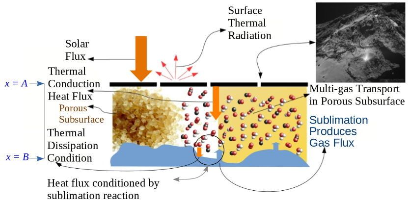
The physical model we present is a refinement of Whipple’s (1950) icy conglomerate model, enhanced to include the presence of a non-volatile, low conductivity porous mantle (see Figure 1). In active comets, such a “rubble mantle” is produced by fallback of suborbital particles and by volatile loss from the strongly heated surface. In inactive comets, for example those in the Oort cloud and Kuiper belt storage reservoirs, an irradiation mantle can grow as pure ices are rendered non-volatile by prolonged exposure to cosmic rays (Kaiser & Roessler (1997), Abplanalp, Frigge, & Kaiser (2019), Gautier et al. (2019)). In our model, we assume that a non-volatile mantle of variable thickness and porosity overlies CO ice.
In equilibrium with sunlight, the energy balance averaged over the surface of a spherical, isothermal nucleus is written as
| (1) |
The first term on the left of Equation (1), in which is the solar constant, is the heliocentric distance in AU and is the bond albedo, represents the absorbed solar power. The second term on the left, only important at the largest heliocentric distances, accounts for heating of the nucleus from other external sources. These include the cosmic microwave radiation background and the integrated light of the stars, as represented by an effective temperature = 10 K. The emissivity of the nucleus is while is the Stefan-Boltzmann constant. On the right, the first term is the flux of radiation from the nucleus surface at temperature, , while the second term is the conducted flux. There is no contribution from sublimation since the surface layers are assumed to be volatile-free.
| (2) |
where the first term, , is the effective thermal conductivity of the porous mantle and second term accounts for radiative conductivity. is an empirical attenuation factor for radiative conduction of void and adjacent grain surfaces within the porous medium.
As shown schematically in Figure (1), the ice is not on the surface as in Whipple’s model but hidden under a mantle. Energy propagated through the mantle to deeper layers can trigger the sublimation of buried ices. At the ice-mantle interface, the conducted energy flux sublimates ice at rate
| (3) |
in which we ignore heat conducted into the “cold core” beneath the sublimation front. A justification of this neglect is given in the Appendix.
Here, the sublimation is entirely controlled by the conducted heat; a non-equilibrium process. The generated gas is also subject to another non-equilibrium process caused by the pressure gradient. The heat is driven down the temperature gradient towards the ice front, in Figure (1), while the gas is driven up towards the surface of the comet, , by the pressure gradient established in the porous medium. In this simple comet model the reverse flow of molecules is not favored, so condensation is somewhat unlikely and is neglected for simplicity. The sublimation flux that has been calculated in Watson & al. (1961) and in Delsemme, & Miller (1971) approximates the sublimation flux in our case too. Otherwise, we should model the condensation process and calculate the net flux
| (4) |
Practically, is an upper limit to the sublimated flux because of the possibility of back-flow and sticking of molecules reflected from particles above the ice front. This is the necessary Neumann boundary condition. At all levels above the ice front, we calculate the net flux, , formed as molecules diffuse through the porous medium.
In equation (4), is the equilibrium pressure of the gas over the ice as function of temperature. contains valuable information about both the gas and the ice structure. We consider sublimation and condensation as facets of a single process which is a first order phase transition phenomenon. It is worthwhile to invoke the chemical reaction formalism to address it. Sublimation is considered as the direct process while condensation is the reverse process; analogous to the direct and reverse arrows between reactants and products in chemical reaction theory. Usually, experiments are conducted in closed thermodynamic equilibrium to characterize the chemical reaction and find the equilibrium constant called . We found that for pure ice, the temperature dependence of varies just like in the language of chemical reactions. The resulting pressure relation resembles the Arrhenius equation (5). Physically, the similarity arises because in a chemical reaction we consider the breakage of bonds within molecules while, in sublimation, the breaking bonds are those between molecules. For this reason, the activation energies in the sublimation case are small compared to the energies involved in chemical reactions.
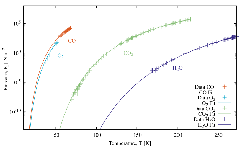
We fitted the sublimation data from Fray & Schmitt (2009) using
| (5) |
where is the molar gas constant, is the activation energy of sublimation, and is a constant, using a non-linear Levenberg Marquardt technique. The data and the fits are shown in Figure (2).
Equation (5) provides a better fit to the data than the polynomials used by Fray & Schmitt (2009). We succeeded in inferring the activation energy of with an exceptional accuracy, see the energies actually measured using various dedicated experimental methods and we did this independently and in a temperature range not included in the data (Luna & al., 2014).
Our model is governed by two coupled partial differential equations, one for heat transport
| (6) |
and one for mass transport
| (7) |
In Equation (6) is the density and is the conductivity at temperature, , while is the time and is the depth in the nucleus, and (see equations 8 and 9) is the heat capacity of the mantle. In Equation (7), is the Knudsen diffusion coefficient, is the thermal speed, the permeability of the porous medium (Cussler, 2009), and is the dynamic viscosity. Other quantities are , the Boltzmann constant, , a numerical constant on the order of 1, , the temperature, the CO molecule’s collision diameter and the CO molecular mass, , the CO gas pressure , is the molecular density of CO; the pore radius, is the porosity.
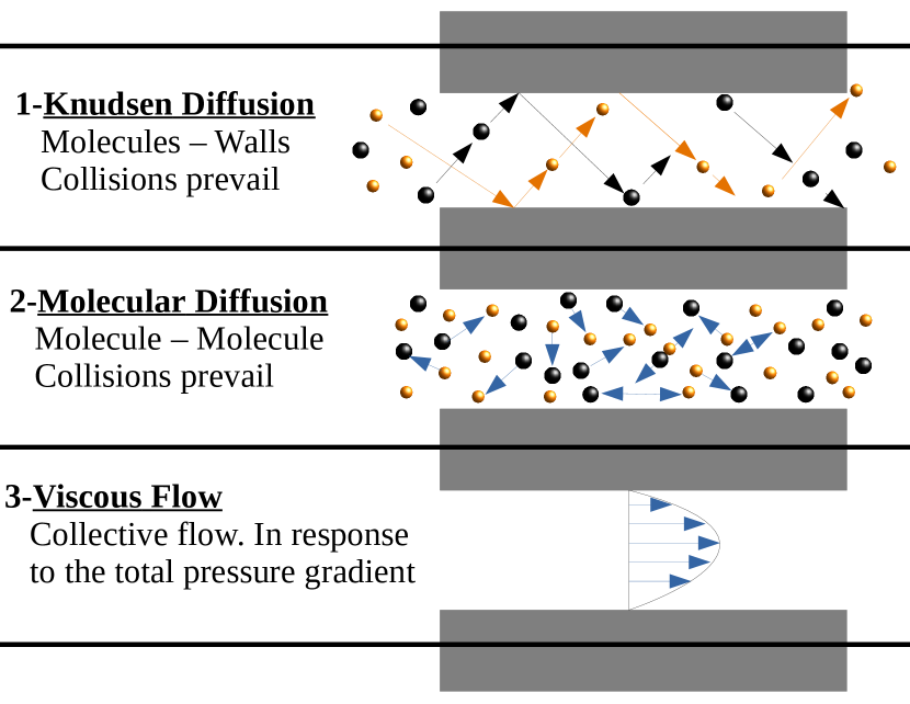
The equations are coupled by the transport coefficients. Water ice acts as a mineral at the low temperatures found in the outer solar system, so we neglect the H2O gas flux and focus only on the CO flux using a simplified version of the model described in Bouziani & Fanale (1998). Gas produced by sublimation passes through the porous mantle towards the comet surface. Figure (3) illustrates the various modeled mechanisms of gas transport inside the porous mantle. This model takes into account both microscopic and macroscopic behavior and also treats the interaction between the gas and the walls. It provides a continuous physical modeling of the coupling between mechanisms - from discontinuous collisions to the collective macroscopic behavior of continuous matter - and thus for the prediction of the mass flow rate and pressure distribution with reasonable accuracy over the widest range of gas pressures. The model depends only on molecular data and fundamental parameters such as temperature, composition and total pressure. This approach allows us to address the thermal and dynamical coupling of comets in a continuous and physical way. Table (1) summarizes parameters used in the numerical simulations.
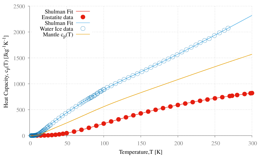
We assume that the dust mantle is composed of a mixture of refractory minerals and water ice. To estimate the heat capacity of the ice, we use the heat capacity (J kg-1 K-1)deduced from the data provided in Shulman (2004).
| (8) |
For the refractory part of the mantle we use the data for Enstatite found in Krupka & al (1985) and we find that the Shulman equation gives an excellent representation of the data at both high and low temperatures;
| (9) |
We assume a water ice/dust ratio = 1, and thus take the specific heat capacity of the mixture as the average of equations (9) and (8). Figure (4) shows how the heat capacity of the mantle depends on the temperature.
We solved Equations (6 & 7) as a function of time, following the motion of comet C/2017 K2 upon its approach to the Sun from large heliocentric distances. For this purpose, we used the barycentric orbital elements from Królikowska & Dybczyński (2018) while noting that the current Sun-centered orbit from NASA’s Horizons ephemeris software111http://ssd.jpl.nasa.gov/horizons.cgi is slightly hyperbolic (eccentricity = 1.0004, vs. = 0.9999 from Królikowska & Dybczyński (2018)). This difference between the barycentric and Sun-centered elements is negligible for our purposes. The model solves the heat and gas transport equations in a coupled manner. As it approaches the Sun, the surface temperature of C/2017 K2 increases from the limiting interstellar value of 10 K to higher temperatures, creating a temperature gradient within the mantle, and driving conduction towards the buried ice layer. Heating of the ice triggers sublimation, producing a pressure gradient and resulting in a diffusive flow of gas towards the comet’s surface, eventually leading to escape and the expulsion of embedded dust particles through gas drag. The downward conduction of heat and the upward transport of sublimated gas molecules are characterized by distinct and different timescales, each dependent on the thermal and micro-physical properties of the material, as we will discuss in Section (3.2). The boundary condition (Equation 1) is time-dependent because the orbital position is a function of time.
3 Results & Discussion
3.1 The Activity Mechanism
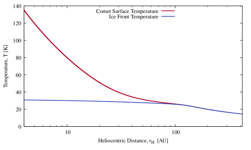
Figure (5) shows that the surface temperature increases, as expected from radiative equilibrium, in proportion to . On the other hand, the temperature at the ice-mantle boundary at first rises as decreases (we refer to this region as Regime 1) but becomes nearly constant at 150 AU (Regime 2). This flattening occurs because the heat conducted to the ice-mantle boundary in Region 2 is almost entirely used to break intermolecular bonds in the ice, leaving little to raise the temperature. These qualitatively different temperature vs. distance trends were first noted for H2O by Mendis & Brin (1977) for Comet Kohoutek (1973f) and later by Prialnik & Bar-Nun (1988). The model confirms this behavior and extends it to much larger heliocentric distances in more volatile ices. For convenience, in the remainder of this paper we refer to the junction between Region 1 and Region 2 as the “Mendis point”. The CO flux coming out from the comet mantle is given by Equation (7). In order to better understand the orbital behavior of this flux as the comet approaches the sun, we solve the coupled equations (6 & 7) and focus on the averaged flux by estimating the difference in the value of a variables between the surface of the comet and the base of the mantle , this approximation is emphasized next in section (3.2); doing so, we deliberately ignore the local variation of this flux within the mantle. The flux is
| (10) |
Equation (10) shows how Knudsen free diffusion combines with collective viscous flow (also called Hagen-Poiseuille flow in fluid dynamics). Although these two flows are additive, they are not independent of each other. They are coupled through the pre-gradient coefficients, thanks to the microscopic approach of the model which integrates the walls in the collision from the very beginning.
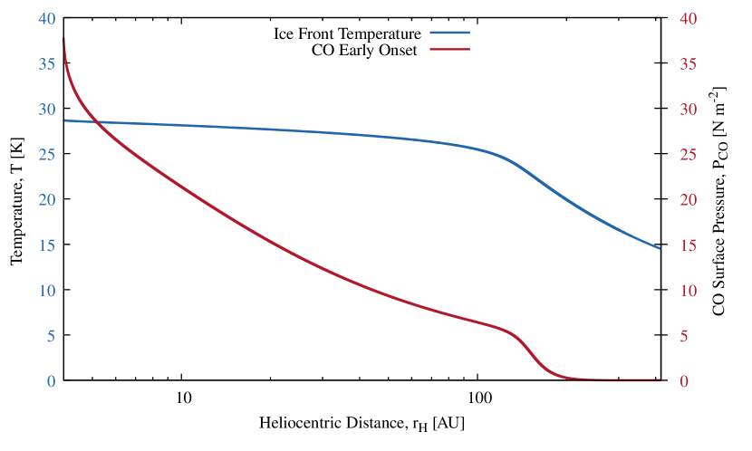
Figure (6) shows the CO gas pressure just below the surface, , as a function of . We find a prominent local bump in at AU, corresponding to the Mendis point. Further exploration shows that the location and amplitude of the bump depend on several physical parameters, including the assumed active surface fraction of the mantle (the comet surface structure) and the mantle thickness.
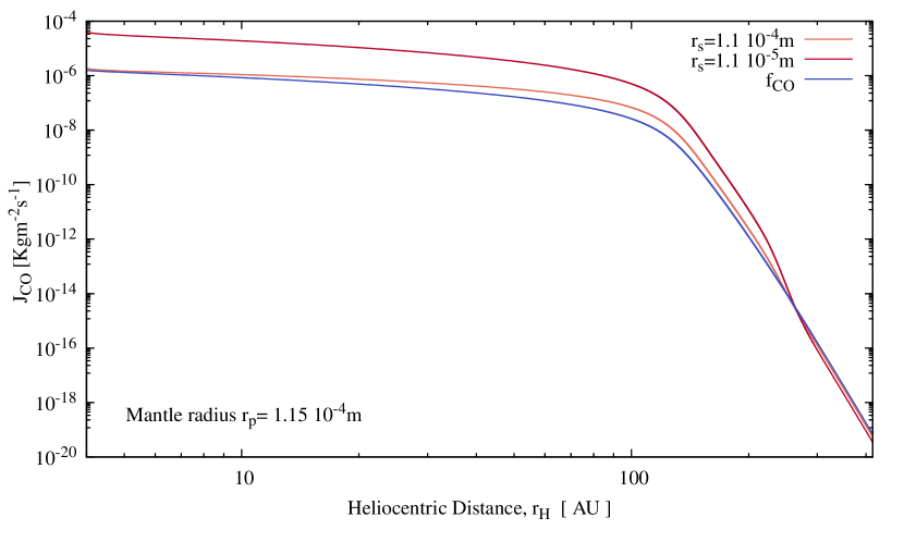
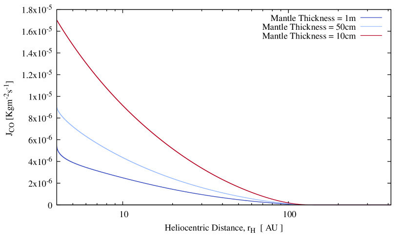
For example, Figure (7) shows that the amplitude of the Mendis point bump increases as the mantle active surface fraction decreases, because a lower surface pore radius, , increases the gas speed and allows the build up of higher pressures that in turn speed up even more the flux (viscous mode is more rapid). Figure (8) shows as expected that flux increases as the mantle thickness decreases; while thinner mantles provide less impedance to the flow of gas, they also allow higher temperatures, and so higher pressures, at the ice sublimation front.
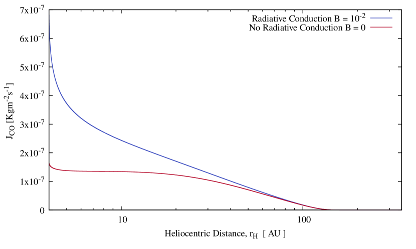
The steady increase in after the 150 AU Mendis point becomes an abrupt rise as the comet approaches the Sun (c.f. Figure 9). Part of this strong increase at small is due to the rising contribution of the radiative term to the effective thermal conductivity of the mantle. To demonstrate this behavior, we show in Figure (9) the effect of arbitrarily removing the radiative term by setting = 0 in Equation (2). In this model with a 5m thick mantle, the CO flux at 4 AU falls from kg m-2 s-1 (blue curve, including radiative term) to kg m-2 s-1 (red curve, no radiative term).
Figures (6, 7, 8 & 9) reveal that, depending on assumed parameters of the mantle, radiative conduction begins to be significant around AU, reaches its maximum near perihelion but has no effect at distances corresponding to the CO Mendis point.
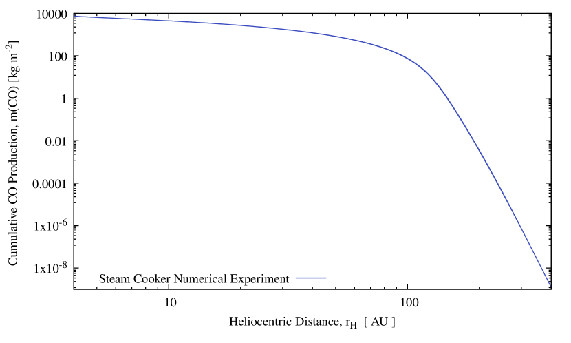
Why is there a local pressure bump near = 150 AU (c.f. Figure 6), and not a continuous rise towards smaller heliocentric distances? Our models give several clues. First, consider the unlikely case of a totally sealed comet surface (the “steam cooker” approximation). Figure (10) shows that, as expected, the calculated pressure closely follows the temperature of the ice with no pressure bump and independent of the adopted physical parameters of the mantle. This numerical experiment gives the total cumulative CO gas production on the whole path, mainly produced after the CO Mendis point. The steam cooker approximation proves that the bump and changes inward of the Mendis point are products of gas transport processes in the mantle because these fall to zero when the surface is sealed. Second, apart from this pathological case, which we do not expect to find in nature, the pressure bump exists in all models, albeit with widely different amplitudes depending on the model parameters, even in the case of an almost totally (99%) permeable mantle.
Prialnik & Sierks (2017) noted that the uppermost surface layer of the mantle may be less permeable to flow than the deeper layers. We model this by reducing the comet surface pore radii, , compared to the mantle pore radii, . Figure (7) shows that the flux amplitude and behavior is strongly controlled by the assumed structural properties of the comet mantle. The more the flux is inhibited, the higher is the flux bump. The location of the Mendis point at the junction between the two thermal regimes was noted above. It is at this confluence point that the lower flow entering the mantle, ( in Figure 1) stops increasing over time and slowly becomes constant in response to the flattening of the temperature dependence caused by strong CO sublimation in Regime 2. This happens while, at the surface of the comet ( in Figure 1), and also in the mantle depending on the pore radius, the gas pressure remains high. The transition from the rising ice front temperature in Regime 1 to the nearly constant ice front temperature in Regime 2 leads to a temporary under-supply of CO at the base of the mantle, relative to the loss rate from the surface, creating a local maximum as in Figure (6) or less visible but there in the orange curve of Figure (7). The width of the bump is a measure of the mantle’s holding or response time. The under-supply of CO starting around 150 AU, relative to the rate of loss from the surface, is responsible for the peak as the mantle switches from regime 1 to regime 2.
3.2 Retention Time Scale
The porous mantle of the comet acts as a buffer to the gas flow produced by sublimation at the bottom. In order to understand this buffer and explore the physical parameters that affect the gas retention time, we estimate in this section the time scale corresponding to this buffer.
We first define the Knudsen Number by
| (11) |
where is the pore radius and the mean free path is given by
| (12) |
Here, is the effective particle radius and is the number density in the gas. The Knudsen number gives a measure of the importance of gas - gas collisions relative to gas - particle collisions with the solid material making up the porous mantle.
We define an effective flow velocity of the CO gas through the mantle, , from , where is the gas number density. Then, if is the mantle thickness, Equation (10) can be rewritten as
| (13) |
The time taken for the flow to cross defines a holding or retention timescale, . Equation (13) gives
| (14) |
Here and are the differences in pressure and gas density, respectively, between the surface of the comet (level A in Figure 1) and the bottom of the mantle (level B). For simplicity, we calculate the intermediate coefficients , and of this equation, using the averaged value of temperature, molecular density and pressure (i.e. ).
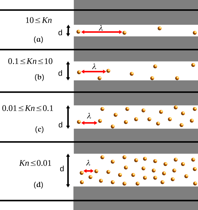
Equation (14) shows that is governed by the two main modes of gas transport, namely 1) Knudsen diffusion in the second denominator term and 2) viscous flow (first denominator term). Figure (11) illustrates these two modes as well as the intermediate transition and slip stages that are intermediate steps between them over the wide range of pressures and pore sizes. The Knudsen number approximately indicates the ranges of the different modes.
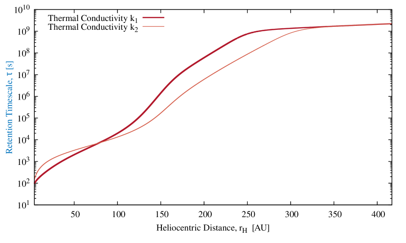
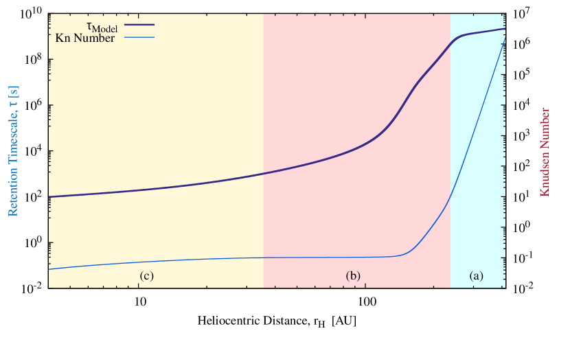
At what heliocentric distance does the Knudsen-Viscous transition occur? The answer will depend on the structure of the dust mantle, in particular the pore radius and the average free path, , which varies with pressure. Figure (12) shows how the retention time changes with the heliocentric distance, , focusing on the coupling between the Knudsen flow and the viscous flow and the different steps between the two flows. It reveals two very distinct configurations. At large we find an almost constant time scale of one century, leading to a slow and almost uniform motion of the gas leaving the comet surface at a global bulk flow velocity of V = (m ). The retention time scale decreases dramatically as the comet approaches the sun, falling to about an hour at 50 AU. This indicates an acceleration of the gas, which we approximate by estimating the slope of the Figure (12), given the assumed physical parameters. By examining the behavior of the retention time Figure (13), we can easily identify the four known modes for each independently computed Knudsen number value and this is then a check of the model. The model was able to capture the complete physics of the flow without any artificial intervention by using the Knudsen number to switch from one mode to the other.
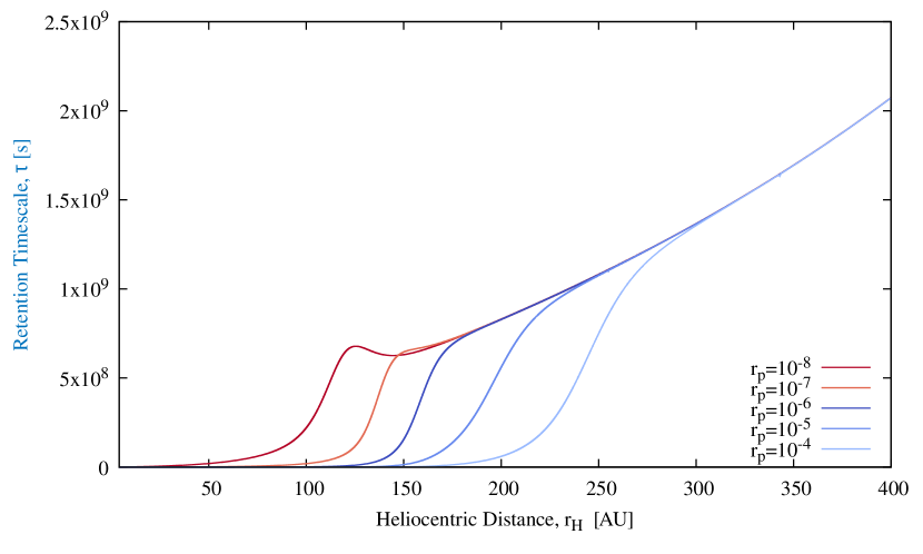
Knudsen diffusion predominates mainly at low pressure and the model allows a viscous flow to develop continuously when the pressure becomes appreciable. As we produce gas by sublimation, Figures (14) show that depending on the transport mode, the duration of this retention time can vary widely.
3.3 Largest ejected dust particle
To be ejected, a dust particle must first overcome cohesive forces, , exerted on it by the surrounding dust material (Gundlach et al., 2015). The minimum size of grains that could escape is (Jewitt et al., 2019a):
| (15) |
where is a dimensionless constant of order unity, (kg m-2 s-1) is the mass sublimation flux and is the speed of the sublimated gas. Once detached, the dust grain needs a force to accelerate above escape velocity. This force can be provided by gas drag. For particles that are spherical and of uniform density, the maximum size of grains that can be ejected is approximated by (Jewitt et al., 2019a):
| (16) |
Here & are the dust grain sizes escaping the comet surface against cohesive forces and against cometary gravity, respectively. The model outputs : and are respectively the CO gas outflow and its thermal speed, taken at the comet surface, where is the comet surface temperature, is the molecular weight, the mass of hydrogen, is the gravitational constant, respectively dust and nucleus densities, is the dimensionless drag efficiency coefficient, assumed to be equal to 1, cohesive strength constant N m-1 (Sánchez & Scheeres, 2014), and is the comet nucleus radius.
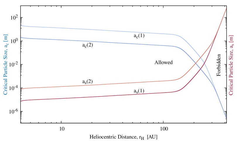
Figure (15) displays Equations (15) and (16) as a function of . Particle radii must lie above the red curve in order for gas drag to exceed inter-grain cohesive forces and below the blue curve for gas drag to exceed the gravitational pull of the nucleus. The Figure shows that these conditions can be simultaneously satisfied at all distances inside the 150 AU CO Mendis point, thus presenting a resolution of the cohesion bottleneck problem for all active comets observed to-date.
4 Summary
We present a detailed gas-physics model of sublimation of cometary CO ice buried beneath a permeable, refractory dust mantle. The model is solved as a function of time and distance along the orbit of the distantly active long-period comet C/2017 K2.
-
1.
Our main result is that we find an unexpected local peak in CO production at very large heliocentric distances ( AU), caused by the build up of pressure beneath a permeable mantle of modest thickness.
-
2.
This peak, whose magnitude is a function of several mantle microphysical parameters, corresponds to the Mendis point, where the buried CO ice front transitions between distinct temperature regimes.
-
3.
While modeled on C/2017 K2 as a specific case, our conclusions are general. Comets entering the solar system from Oort cloud and interstellar distances may become active far beyond the planets, at heliocentric distances 150 AU. Observational attempts to detect such ultra-distant activity are encouraged.
| (1) |
Here, is the thermal conductivity of the material, and are respectively the density and heat capacity.
Quantity is the heating timescale.
The conducted heat flux into the cold core is , where is the temperature difference between the top and bottom of the heated layer of thickness . Then
| (2) |
For comparison, the energy flux used by sublimation is
| (3) |
where is the mass flux of CO in kg m-2 s-1 and J kg-1 is the latent heat of CO from Table (1).
Conduction into the cold core is smaller than sublimation when , leading to
| (4) |
Setting K, W m-1 K-1, = 533 kg m-3, = 119 J kg-1 K-1 and s as the travel time from the Mendis point to 10 AU, we find that sublimation dominates provided kg m-2 s-1. For comparison, Eq. (4) gives kg m-2 s-1 at = 26 K confirming that the sublimation energy flux is much larger than the conducted energy flux.
References
- Abplanalp, Frigge, & Kaiser (2019) Abplanalp, M. J., Frigge, R., & Kaiser, R. I., 2019, SciAdv, eaaw5841
- Baxter et al. (2018) Baxter, E. J., Blake, C. H., & Jain, B. 2018, AJ, 156, 243
- Bouziani & Fanale (1998) Bouziani, N., & Fanale, F. P. 1998, ApJ, 499, 463
- Cussler (2009) Cussler, Edward Lansing, 2009, Diffusion: mass transfer in fluid systems, Cambridge university press
- Delsemme, & Miller (1971) Delsemme, A. H. and Miller, D. C., 1971, Planet. Space Sci., 19, 1229
- Farnham (2021) Farnham, T. 2021, The Astronomer’s Telegram, 14759
- Fray & Schmitt (2009) Fray, N., & Schmitt, B. 2009, Planet. Space Sci., 57, 2053
- Fulle et al. (2020) Fulle, M., Blum, J., & Rotundi, A. 2020, A&A, 636, L3. doi:10.1051/0004-6361/202037805
- Gautier et al. (2019) Gautier, T., Ruf, A., Danger, G., & al., 2019, in EPSC-DPS Joint Meeting 2019, EPSC-DPS2019-914
- Greenberg (1982) Greenberg, J. M., 1982, in IAU Colloq. 61: Comet Discoveries, Statistics, and Observational Selection, ed. Wilkening, L. L., 131
- Guilbert-Lepoutre et al. (2012) Guilbert-Lepoutre, A., Besse, S., Mousis, O., Ali-Dib, M.,Höfner, S., Koschny, D., & Hager, P., 2012, Space Sci. Rev., 197, 271
- Gundlach et al. (2015) Gundlach, B., Blum, J., Keller, H. U., et al. 2015, A&A, 583, A12. doi:10.1051/0004-6361/201525828
- Hui et al. (2019) Hui, M.-T., Farnocchia, D., & Micheli, M. 2019, AJ, 157, 162
- Jewitt (2009) Jewitt, David, . 2009, AJ, 137, 4296
- Jewitt et al. (2017) Jewitt, D., Hui, M.-T., Mutchler, M., et al. 2017, ApJ, 847, L19
- Jewitt et al. (2019a) Jewitt, D., Agarwal, J., Hui, M.-T., et al. 2019a, AJ, 157, 65
- Jewitt et al. (2019b) Jewitt, D., Kim, Y., Luu, J., et al. 2019b, AJ, 157, 103
- Jewitt et al. (2021) Jewitt, D., Kim, Y., Mutchler, M., et al. 2021, AJ, 161, 188. doi:10.3847/1538-3881/abe4cf
- Kaiser & Roessler (1997) Kaiser, R. I., & Roessler, K. 1997, ApJ, 475, 144
- Królikowska & Dybczyński (2018) Królikowska, M., & Dybczyński, P. A. 2018, A&A, 615, A170
- Krupka & al (1985) Krupka, K. M., Robie, R. A., Hemingway, B. S., Kerrick, D. M., & Ito J., 1985, American Mineralogist, 70, 249
- Luna & al. (2014) Luna, R. and Satorre, M. Á. and Santonja, C. and Domingo, M., 2014, A&A, 566, A27
- Mendis & Brin (1977) Mendis, D. A., & Brin, G. D. 1977, Moon, 17, 359
- Moghaddam & Jamiolahmady (2016) Moghaddam, R. N., & Jamiolahmady, M., 2016, Fuel, Elsevier, 173, 298
- Prialnik & Bar-Nun (1988) Prialnik, D. & Bar-Nun, A., 1988, Icarus, 258, V2, 272
- Prialnik & Bar-Nun (1992) Prialnik, D. & Bar-Nun, A. 1992, A&A, 258, L9
- Prialnik & Sierks (2017) Prialnik, D. and Sierks, H., 2017, MNRAS, 469, S217
- Sánchez & Scheeres (2014) Sánchez, P., & Scheeres, D. J. 2014, Meteoritics and Planetary Science, 49, 788
- Shulman (2004) Shulman, L. M. 2004, A&A, 416, 187
- Watson & al. (1961) Watson, K. and Murray, B. C. and Brown, H., 1961, J. Geophys. Res., 66, 9, 3033
- Whipple (1950) Whipple, F. L. 1950, ApJ, 111, 375
| Parameters | Symbols | Values | References |
|---|---|---|---|
| Oort Cloud Temperature (K) | Baxter et al. (2018) | ||
| Gravitational Constant ( ) | |||
| Comet Nucleus Surface Albedo | |||
| Comet Nucleus Radius (m) | Jewitt et al. (2017) | ||
| Comet Nucleus Density (kg m-3) | |||
| Dust Grains Density (kg m-3) | |||
| Porous Crust Thickness (m) | – | ||
| Main Pore Radius (m) | – | ||
| Porosity | 0.80 | ||
| Emissivity | |||
| Stefan-Boltzmann Constant (W m-2 K-4 ) | |||
| Solar Constant (W m-2 ) | |||
| Boltzmann Constant (J K-1 ) | |||
| Ideal Gas Constant (J K-1 mol-1 ) | |||
| Latent Heat–CO (J mol-1) | Data & Fits Fig. (2) | ||
| Sublimation Pressure of CO (N m-2) | Data & Fits Fig. (2) | ||
| Thermal Conductivity (W m-1 K-1) | & - | Mendis & Brin (1977) |