warn luatex=false
Collisional Approach for Open Neutrino Systems
Abstract
We develop a collisional framework for neutrino propagation within open quantum systems, termed the Collisional Approach for Open Neutrino Systems (CAONS). A Born-Markov equation is derived, linking decoherence, dissipation, decay rates, and scattering cross sections. Perturbation theory is not required and the resultant master equation is applied to visible and invisible neutrino decays and propagation through a stationary medium. Comparing with previous studies on neutrino decoherence, we show that current bounds on decoherence parameters can significantly tighten constraints on neutrino couplings with dark-matter. Lastly, we establish connections between CAONS and non-Hermitian Hamiltonian approaches.
I Introduction
The neutrino as an Open Quantum System (OQS) offers a novel approach to explore physics beyond the Standard Model (SM) [1, 2, 3]. A key motivation for applying the OQS framework in neutrino physics is its ability to transform pure neutrino states into mixed states, i.e., from a single vector state into a statistical mixture. This loss of purity entails entropy production and irreversibility, unlike standard neutrino oscillation models, where purity is preserved.
The first application of the OQS framework to neutrinos dates back to the late 1990s, providing an alternative explanation for the atmospheric muon neutrino deficit [4]. That same year, Sun and Zhou [1] explored gravity effects and black hole evaporation as motivations for employing OQS in neutrino physics.
The time evolution of systems weakly coupled to a memoryless environment — where interactions are independent of previous events — is described by the Born-Markov master equation. When diagonalized, it yields the Gorini-Kossakowski-Sudarshan-Lindblad equation (Lindblad equation) [5, 6]. In 2000, Lisi et al. [2] applied the Lindblad equation to neutrino phenomenology, proposing that the Super-Kamiokande experiment could detect decoherence effects caused by unknown physics, such as quantum gravity. Lacking a physical model for a microscopic derivation, they introduced ad hoc decoherence parameters proportional to powers of the neutrino energy, assuming energy conservation and no dissipation.
While decoherence can reveal new physics, it may also affect measurements of standard oscillation parameters, including the CP-violation phase and the mixing angle [7, 8]. Thus, the OQS approach is crucial not only for probing new interactions but also for correctly interpreting neutrino oscillation data. In neutrino physics, an OQS framework based on scattering theory is especially appealing, as it aligns with quantum field theory—the most advanced framework for particle interactions.
Many studies link neutrino decoherence to quantum gravity [9, 10, 3, 11, 12, 13, 14, 15, 16, 17, 18], using various experiments to constrain the decoherence parameters [8, 15, 10, 19, 20]. However, a microscopic derivation requires an interaction Hamiltonian and the environmental state, which together determine the decoherence and dissipation parameters, denoted generically as [5, 6]. Understanding neutrino propagation can also reveal properties of the environments they traverse, potentially altering interpretations of high-energy neutrino sources.
Different techniques exist to derive master equations. For systems with finite Hilbert spaces, the eigenoperator method is appropriate [5]. For scattering processes, however, the collisional method (or repeated interaction scheme) is often more suitable [21, 22]. We focus on two relevant approaches: i) The first approach considers the complete evolution for a short time interval, , expanding the time evolution operator and tracing over the environment [23]. However, this method introduces an undesirable dependence of on the arbitrary time interval . ii) The second approach, developed by Hornberger and Sipe [21], applies scattering theory to model the evolution of Brownian particles interacting with their environment. They derived a cross section-dependent equation but introduced the unitary part by hand, an unexpected feature since free evolution should arise naturally from the full equation.
In this work, we develop a collisional approach to derive a Born-Markov master equation for neutrinos, termed the Collisional Approach for Open Neutrino Systems (CAONS). This method overcomes the challenges of previous approaches: i) the dependence of the parameters and ii) the arbitrary inclusion of the unitary part. Additionally, unlike most of the existing methods, CAONS is not perturbative, in the sense that the master equation does not come from perturbation theory, and provides a clear interpretation of in terms of scattering cross sections and decay rates. Section II presents the derivation of the CAONS framework. In Section III, we apply it to neutrino decay and scattering. Section IV discusses the implications of our results, followed by final remarks in Section V.
II Collisional Approach for Open Neutrino Systems (CAONS)
In this section, we develop the CAONS framework to study decoherence, particularly in neutrino systems. Although motivated by neutrino propagation, this method is general and can be applied to any particle system subject to decoherence or dissipation.
Let denote the initial state of the composite neutrino-environment system in the Schrödinger picture, with representing the neutrino. Assuming the two systems are initially uncorrelated, we write
| (1) |
where and are the initial density operators of the neutrino and environment, respectively. Given the weak interaction between neutrinos and the environment, the macroscopic state of the environment remains unchanged, and the composite system can be approximated by a product state throughout the evolution—an assumption known as the Born approximation [6]. We focus on free particles and vacuum environments, so commutes with the free Hamiltonian.
After evolving for a time interval , the state becomes
| (2) |
where is the time-evolution operator. In the interaction picture, Eq. (2) transforms into
| (3) |
where is the scattering matrix for non-negative times, defined as
| (4) |
with denoting the time-ordering operator and the interaction Hamiltonian coupling the system and environment.
Expanding , where is the non-negative time transfer matrix, we obtain
| (5) |
It is important to note that we choose in Eqs. (2)–(5) to be small compared to the system’s evolution timescale but large compared to the interaction time. This ensures that the upper limit of the time integral in , and consequently in , can extend to , introducing the Markov approximation. This approximation enables us to compute the matrix elements of similarly to the standard transfer matrix . Specifically, instead of
| (6) |
we obtain
| (7) |
where P.V. denotes the Cauchy principal value.
Since is unitary, i.e., , it follows that
| (8) | ||||
| (9) |
Applying these results to Eq. (5) and dividing by , we obtain
| (10) |
Taking the limit and reverting to the Schrödinger picture, then performing a partial trace over the environment, we find
| (11) |
where is the free Hamiltonian of the neutrino, and
| (12) |
with being the time-evolution operator for the free neutrino and denoting the average over the environment states. In Eq. (11),
| (13) |
Although is defined as in Eq. (13), it requires corrections to ensure unitarity. Specifically, the imaginary part must satisfy , where is the Lamb-shift Hamiltonian. Thus, we redefine and include in the unitary part of the evolution.
There are three key points regarding the master equation: i) The initial time is arbitrary, so the equation must hold for any . ii) Although in and appears divergent, it is regularized in and governs the emergence of probability rates in the dissipator. iii) Unlike standard Born-Markov equations, our result is not perturbative by default, though perturbation theory can be applied to the dissipation and decoherence parameters derived later.
To express the master equation using operators acting solely on neutrino states, we solve the trace over the environment. Let be a complete set of orthonormal states for the environment, with labels and for environment states, and and for neutrino states. These labels fully specify the system; for instance, denotes a neutrino with momentum and state , whether in the flavor or mass basis. This notation applies to states with any number of particles.
Assuming a diagonal density operator for the environment:
| (14) |
we solve the partial trace and apply the rotating wave approximation [5, 6] to eliminate fast oscillatory terms. The resulting dissipator is:
| (15) |
where the operators and parameters are defined as:
| (16) |
| (17) |
The parameters are probability rates averaged over the environment, with representing the transition probabilities.
We emphasize that parameters can be interpreted in terms of decay and scattering rates due to their connection with transition probabilities. CAONS fully determines the master equation structure, requiring only the probability rates to compute the neutrino time evolution within this framework.
Next, we briefly discuss and . The Lamb-shift Hamiltonian, , introduces a small correction to the system’s energy levels [5]. It commutes with the free Hamiltonian and has no significant influence on the evolution a priori. Thus, we absorb into the free Hamiltonian in this study.
Focusing on , we expand to first order using Eq. (12):
| (18) |
Thus, corresponds to the matter potential in neutrino propagation, similar to the case of solar neutrinos [24].
II.1 Evolution of a Subspace
We now compute the time evolution of each element of , with :
| (19) |
The master equation yields an infinite set of coupled differential equations due to the combined effects of mass differences and momentum variations, unlike standard treatments focused solely on mass dynamics.
To simplify, we decompose the evolution into subspaces, aligning our formalism with standard approaches. Consider neutrinos with momentum in the subspace , where denotes either mass or flavor states. Let be the projection operator for , and for the complementary subspace.
We focus on scenarios where neutrinos either decay (in)visibly in vacuum or scatter on resting particles. In these cases, neutrinos may leave but cannot return, with the approximation that environmental particles have negligible momentum.
Define the following components:
| (20) |
Using these definitions, the density matrix takes the form:
| (21) |
The differential equations for each block are:
| (22) | ||||
| (23) | ||||
| (24) |
The equation for is the Hermitian conjugate of .
Next, we simplify . With , we find:
| (25) |
Similarly:
| (26) |
since and belong to orthogonal subspaces. Thus, . The master equation for each block simplifies to:
| (27) | ||||
| (28) | ||||
| (29) |
If the momentum superposition is negligible, we take , giving:
| (30) |
This result allows us to disregard in further analysis.
III Basic Applications
This section presents basic applications of the collisional approach, focusing on three examples: i) Neutrino invisible decay: The simplest case, where the neutrino decays to its vacuum state. ii) Neutrino visible decay: The decay results in less energetic neutrinos due to energy-momentum conservation, with final states tending to be less massive. iii) Neutrino scattering on particles at rest: Similar to visible decay, with the neutrino interacting with stationary particles.
For simplicity, we consider a two-family neutrino scenario. The flavor eigenstates, and , are related to the mass eigenstates and by:
| (31) |
The transition probabilities are computed using:
| (32) |
where is the density matrix of a neutrino created in state .
III.1 Neutrino Invisible Decay
Consider a neutrino that decays invisibly. Its interaction Lagrangian is given by [25, 26, 27]:
| (33) |
where includes fields related to the decay. If is a linear combination of mass eigenstates:
| (34) |
the Lagrangian becomes:
| (35) |
We assume a simple model with , where is a fermionic field and is a real scalar. Fig. 1 shows the Feynman diagram for the invisible decay. In a vacuum environment, if is the vacuum state, and the final neutrino state is the vacuum ( in Eq. 17). The total decay rate simplifies to:
| (36) |
where is the total decay rate for a neutrino in state .
For a neutrino created in state , the initial density matrix is:
| (37) |
The evolution of , provided by Eq.(27) is:
| (38) |
where . Thus, the solution is:
| (39) |
The evolved density matrix is:
| (40) |
The survival probability is:
| (41) |
Fig. 2 shows survival probabilities for different decay rates, including the standard case (no decay), , and with . As expected, if both mass eigenstates decay, the survival probability tends to zero as . If only one eigenstate decays, the asymptotic probability equals the initial population of the other mass eigenstate.

III.2 Neutrino Visible Decay
We now consider the visible decay of neutrinos in vacuum. Unlike invisible decay, visible decay changes the proportion of mass eigenstates rather than making neutrinos disappear. Additionally, visible decay alters the neutrino’s momentum, requiring the computation of matrix elements in the subspace.
Assume that a neutrino decays into plus a real scalar. The Lagrangian density is:
| (42) |
The tree-level Feynman diagram is shown in Fig. 3. In this scenario, only decays, so we simplify notation by writing instead of .
Following the same procedure as for invisible decay, we find the evolved density matrix:
| (43) |
The survival probability is:
| (44) |
The asymptotic value of .
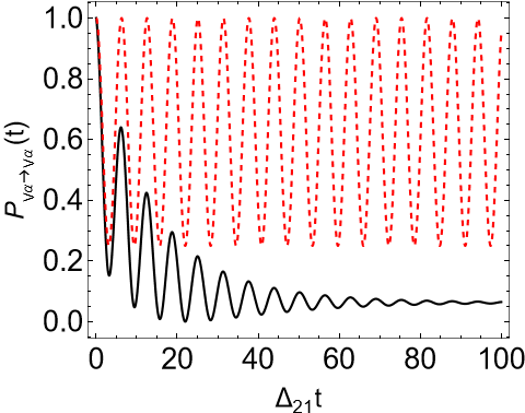
Fig. 4 shows the survival probabilities for this case, including the standard case (no decay) and visible decay with and . As one can see, the probability converges to .
After computing the evolution of , we can compute the evolution for . From Eq. (28), we have:
| (45) |
Since only decays to , we find:
| (46) |
representing the population of neutrinos with mass and momentum .
The fraction in Eq. (46) represents the portion of neutrinos initially in mass eigenstate 2 with momentum that decayed into eigenstate 1 with momentum . In practice, this fraction would be zero due to phase-space considerations. However, experimental measurements have finite precision, so integration over momentum intervals defined by experimental bins is necessary.
III.3 Neutrino Scattering
In this scenario, a neutrino propagates through a homogeneous environment composed of particles at rest. This case combines features from the previous examples: there is suppression of population terms, similar to Eq. (40), but neutrinos remain in the final states. Consider the Lagrangian:
| (47) |
where is a real scalar field. The interaction vertex is shown in Fig. 5.
The matter potential is:
| (48) |
where is the scalar particle mass, and is its number density. We assume , so the interacting eigenstates remain approximately the same as the free ones, but still allow mass-state transitions due to scattering.
The transition probability rates are:
| (49) |
where is the cross section, and is the relative velocity for ultra-relativistic neutrinos. Therefore, for the simple case where all environment particles are at rest, then
| (50) |
The density matrix for the subspace is similar to Eq. (40), but with decay rates replaced by cross sections:
| (51) |
Finally, the matrix elements for are:
| (52) |
which gives the population of neutrinos scattered into different mass eigenstates. This result is valid when ; otherwise, multiple scatterings occur, making it difficult to separate subspaces. However, this provides a useful first approximation for the full master equation.
IV Some Implications
This section discusses indirect implications of our results, including estimates of weak interaction-induced decoherence, limits on neutrino-dark matter coupling constants, and the connection between CAONS and the non-Hermitian Hamiltonian approach.
As noted in Sec. I, early studies modeled decoherence parameters as proportional to some power of the neutrino energy, with bounds determined for different spectral indices. However, as shown in Eq. (17), corresponds to environment-averaged probability rates. For simple environments, such as vacuum or particles at rest, can be expressed in terms of decay rates and cross sections, which often scale with the neutrino energy.
For the analyses in Secs. IV.1 and IV.2, we follow Ref. [20], which offers a detailed study of Earth’s matter density profile. In their model, neutrino dynamics depend on three decoherence parameters expressed as , where is an integer in the range .
IV.1 Weak-Interaction Induced Neutrino Decoherence
As discussed in Sec. III.3, for neutrinos scattering off particles at rest, the decoherence parameter can be expressed as . Using Earth’s density and the sub-TeV neutrino-nucleon cross section [28], we estimate for atmospheric neutrinos traversing the Earth.
The Earth’s average density is , corresponding to a nucleon number density of . The sub-TeV cross section is approximated by [28]:
| (53) |
Thus, using , the decoherence parameter in natural units becomes:
| (54) |
This result aligns with Ref. [29], indicating that most long-baseline experiments are sensitive only to GeV, suggesting that hadronic matter decoherence may not significantly impact these experiments. However, Ref. [20] provides limits for with ranging from GeV to GeV, depending on the scenario. These values suggest that weak interaction-induced decoherence could be comparable to current bounds and should not be disregarded in searches for new physics.
Fig. 6 shows the relation between medium density and the neutrino baseline for different energies and values of , where is described by the Eq.(54). For neutrinos, open dynamics require high-density environments or large objects. In contrast, neutrinos experience decoherence even in stars like the Sun (radius km, average density [30]). Additionally, Ref. [20] suggests that for neutrinos crossing the Earth, , indicating that both matter density and propagation length can be smaller than the values shown in Fig. 6.

IV.2 Interactions with Scalar Dark Matter
Neutrino interactions with ultra-light scalar dark matter, or fuzzy dark matter (FDM), have been studied in [31, 32, 33]. In Ref. [31], interactions are mediated by a neutral fermion of mass , with FDM being either real (self-conjugate) or complex (non-self-conjugate). For real FDM and (Mandelstam variables), the cross section is:
| (55) |
where is the neutrino-FDM coupling constant, and is the neutrino mass. For complex FDM:
| (56) |
where is the FDM particle mass and is the neutrino energy.
Using the local dark matter energy density [34] and the bounds on from Ref. [20], we derive upper limits on the coupling ratios. For complex FDM:
| (57) |
and for real FDM:
| (58) |

Using the results from Ref. [20], Fig. 7 displays the constraints on . While previous studies [31] set the ratio within , our CAONS-based limits are significantly stricter, ranging from to . This highlights the importance of linking decoherence parameters with cross sections to better understand neutrino interactions.
IV.3 Connection with the Non-Hermitian Hamiltonian
The open quantum system (OQS) formalism connects with the non-Hermitian Hamiltonian approach, where:
| (59) |
with governing non-conservative dynamics, commonly used in decay and absorption studies [35].
The Lindblad equation is:
| (60) |
Dropping the first term in the dissipator recovers the same dynamics as the non-Hermitian Hamiltonian:
| (61) |
Thus, contains the same information about interactions and the environment as . Comparing Eq. (61) with Eq. (27), we obtain:
| (62) |
For diagonal , the non-Hermitian and OQS approaches yield similar results. However, for non-diagonal , the OQS method requires solving (likely coupled) equations, whereas the non-Hermitian approach only requires equations. Using Eqs. (61) and (62), the Hamiltonian can be expressed as:
| (63) |
After diagonalizing , we get:
| (64) |
Thus, CAONS provides a tool for uncovering the microscopic meaning of , as it directly relates to transition probability rates.
V Conclusions and Final Remarks
Using quantum scattering theory, we derived a general Born-Markov master equation, linking the parameters to decay rates and cross sections. The resulting equation is not perturbative, setting it apart from most methods in the literature. A key advantage of the CAONS framework is its flexibility: can be computed from interaction models and environmental particle profiles or inferred from phenomenological transition rates, making it especially useful when kinematics play a central role.
The CAONS framework enables precise determination of neutrino time evolution, decay rates, and energy dissipation through scattering processes. Additionally, the relation between and cross sections provides valuable insights into neutrino-environment interactions. One important finding is that decoherence caused by hadronic matter lies within established limits, highlighting the need to account for it when searching for non-standard neutrino interactions. If neutrino decoherence is observed, contributions from hadronic matter must be considered to accurately estimate the effect of non-standard interactions.
We also applied the CAONS framework to constrain the coupling between neutrinos and ultra-light dark matter. Current limits on yield a much stricter constraint on , with for complex (real) scalar dark matter—tightening the bound by at least 15 orders of magnitude compared to previous studies. This demonstrates the framework’s power in refining our understanding of neutrino interactions.
Finally, we showed how CAONS connects to the non-Hermitian Hamiltonian method, useful for studying irreversible particle disappearance. This connection underscores CAONS’s potential to enhance the application of non-Hermitian approaches across various contexts.
VI Acknowledgements
We would like to thank A. de Gouvêa for his comments and careful reading of the paper. This study was financed in part by the Coordenação de Aperfeiçoamento de Pessoal de Nível Superior - Brasil (CAPES) - Finance Code 001.
References
- Sun and Zhou [1998] C. P. Sun and D. L. Zhou, Quantum decoherence effect and neutrino oscillation (1998), arXiv:hep-ph/9808334 .
- Lisi et al. [2000] E. Lisi, A. Marrone, and D. Montanino, Probing possible decoherence effects in atmospheric neutrino oscillations, Physical Review Letters 85, 1166 (2000).
- Hooper et al. [2005] D. Hooper, D. Morgan, and E. Winstanley, Probing quantum decoherence with high-energy neutrinos, Physics Letters B 609, 206 (2005).
- Grossman and Worah [1998] Y. Grossman and M. P. Worah, Atmospheric muon-neutrino deficit from decoherence (1998), arXiv:hep-ph/9807511 .
- Breuer et al. [2002] H.-P. Breuer, F. Petruccione, et al., The theory of open quantum systems (Oxford University Press on Demand, 2002).
- Schlosshauer [2007] M. A. Schlosshauer, Decoherence: and the quantum-to-classical transition (Springer Science & Business Media, 2007).
- Coelho et al. [2017] J. A. Coelho, W. A. Mann, and S. S. Bashar, Nonmaximal 23 mixing at nova from neutrino decoherence, Physical review letters 118, 221801 (2017).
- Carpio et al. [2018] J. Carpio, E. Massoni, and A. Gago, Revisiting quantum decoherence for neutrino oscillations in matter with constant density, Physical Review D 97, 115017 (2018).
- Gago et al. [2002] A. Gago, E. M. Santos, W. J. d. C. Teves, and R. Z. Funchal, A study on quantum decoherence phenomena with three generations of neutrinos, arXiv preprint hep-ph/0208166 (2002).
- Fogli et al. [2003] G. Fogli, E. Lisi, A. Marrone, and D. Montanino, Status of atmospheric neutrino → oscillations and decoherence after the first k2k spectral data, Physical Review D 67, 093006 (2003).
- Barenboim and Mavromatos [2005] G. Barenboim and N. E. Mavromatos, Cpt violating decoherence and lsnd: A possible window to planck scale physics, Journal of High Energy Physics 2005, 034 (2005).
- Morgan et al. [2006] D. Morgan, E. Winstanley, J. Brunner, and L. F. Thompson, Probing quantum decoherence in atmospheric neutrino oscillations with a neutrino telescope, Astroparticle Physics 25, 311 (2006).
- Fogli et al. [2007] G. Fogli, E. Lisi, A. Marrone, D. Montanino, and A. Palazzo, Probing nonstandard decoherence effects with solar and kamland neutrinos, Physical Review D 76, 033006 (2007).
- Mavromatos et al. [2008] N. E. Mavromatos, A. Meregaglia, A. Rubbia, A. S. Sakharov, and S. Sarkar, Quantum-gravity decoherence effects in neutrino oscillations: Expected constraints from cngs and j-parc, Physical Review D 77, 053014 (2008).
- Sakharov et al. [2009] A. Sakharov, N. Mavromatos, A. Meregaglia, A. Rubbia, and S. Sarkar, Exploration of possible quantum gravity effects with neutrinos i: Decoherence in neutrino oscillations experiments, in Journal of Physics: Conference Series, Vol. 171 (IOP Publishing, 2009) p. 012038.
- Capolupo et al. [2019] A. Capolupo, S. M. Giampaolo, and G. Lambiase, Decoherence in neutrino oscillations, neutrino nature and cpt violation, Physics Letters B 792, 298 (2019).
- Buoninfante et al. [2020] L. Buoninfante, A. Capolupo, S. M. Giampaolo, and G. Lambiase, Revealing neutrino nature and cpt violation with decoherence effects, The European Physical Journal C 80, 1 (2020).
- Hellmann et al. [2021] D. Hellmann, H. Päs, and E. Rani, Searching new particles at neutrino telescopes with quantum-gravitational decoherence, arXiv preprint arXiv:2103.11984 (2021).
- Gomes et al. [2017] G. B. Gomes, M. Guzzo, P. De Holanda, and R. Oliveira, Parameter limits for neutrino oscillation with decoherence in kamland, Physical Review D 95, 113005 (2017).
- Coloma et al. [2018] P. Coloma, J. Lopez-Pavon, I. Martinez-Soler, and H. Nunokawa, Decoherence in neutrino propagation through matter, and bounds from icecube/deepcore, The European Physical Journal C 78, 1 (2018).
- Hornberger and Sipe [2003] K. Hornberger and J. E. Sipe, Collisional decoherence reexamined, Physical Review A 68, 012105 (2003).
- Hornberger [2009] K. Hornberger, Introduction to decoherence theory, Entanglement and Decoherence: Foundations and Modern Trends , 221 (2009).
- Ciccarello et al. [2022] F. Ciccarello, S. Lorenzo, V. Giovannetti, and G. M. Palma, Quantum collision models: Open system dynamics from repeated interactions, Physics Reports 954, 1 (2022).
- Giunti and Kim [2007] C. Giunti and C. W. Kim, Fundamentals of neutrino physics and astrophysics (Oxford university press, 2007).
- Pasquini and Peres [2016] P. Pasquini and O. Peres, Bounds on neutrino-scalar yukawa coupling, Physical Review D 93, 053007 (2016).
- Choubey et al. [2021] S. Choubey, M. Ghosh, D. Kempe, and T. Ohlsson, Exploring invisible neutrino decay at essnusb, Journal of High Energy Physics 2021, 1 (2021).
- Gelmini and Valle [1984] G. B. Gelmini and J. W. Valle, Fast invisible neutrino decays, Physics Letters B 142, 181 (1984).
- Formaggio and Zeller [2012] J. A. Formaggio and G. P. Zeller, From ev to eev: Neutrino cross sections across energy scales, Reviews of Modern Physics 84, 1307 (2012).
- Nieves and Sahu [2020] J. F. Nieves and S. Sahu, Neutrino decoherence in an electron and nucleon background, Physical Review D 102, 056007 (2020).
- Factbook [1999] T. P. Factbook, Density of the sun (1999).
- Barranco et al. [2011] J. Barranco, O. G. Miranda, C. A. Moura, T. I. Rashba, and F. Rossi-Torres, Confusing the extragalactic neutrino flux limit with a neutrino propagation limit, Journal of Cosmology and Astroparticle Physics 2011 (10), 007.
- Sen and Smirnov [2023] M. Sen and A. Y. Smirnov, Refractive neutrino masses, ultralight dark matter and cosmology, arXiv preprint arXiv:2306.15718 (2023).
- Huang and Nath [2022] G.-y. Huang and N. Nath, Neutrino meets ultralight dark matter: 0 decay and cosmology, Journal of Cosmology and Astroparticle Physics 2022 (05), 034.
- Sofue [2020] Y. Sofue, Rotation curve of the milky way and the dark matter density, Galaxies 8, 37 (2020).
- Moiseyev [2011] N. Moiseyev, Non-Hermitian quantum mechanics (Cambridge University Press, 2011).