Collective steady-state patterns of swarmalators with finite-cutoff interaction distance
Abstract
We study the steady-state patterns of population of the coupled oscillators that sync and swarm, where the interaction distances among oscillators have finite-cutoff in interaction distance. We examine how the static patterns known in the infinite-cutoff are reproduced or deformed, and explore a new static pattern that does not appear until a finite-cutoff is considered. All steady-state patterns of the infinite-cutoff, static sync, static async, and static phase wave are respectively repeated in space for proper finite-cutoff ranges. Their deformation in shape and density takes place for the other finite-cutoff ranges. Bar-like phase wave states are observed, which has not been the case for the infinite-cutoff. All the patterns are investigated via numerical and theoretical analysis.
Swarming [1] is the collective behavior of biological/artificial entities in the absence of centralized coordination. Interaction between agents is the reason for the behavior, and thus its modeling is a core task to understand or control the emergent phenomena. Recently, a steady state pattern was studied [2] for the overdamped limit model with potential while motivated by biological aggregations in viscous liquid, and the static feature later becomes various [3] as self-propelling factor is implemented through the phase dynamics of synchronization [4]. The interaction therein is mediated by a potential function that may change in time. We here consider the cutoff of interaction distance to model the fact that the distance any living/engineering entities can manage is necessarily finite. The previously understood static feature lasts till the cutoff is larger than the size of the pattern formed in the absence of cutoff. For the smaller cutoff, the pattern is deformed in an explainable manner, and then it becomes amorphous or non-stationary for further decrease. A new class of static structures not appearing in the no-cutoff model is observed and specified. Phase diagram for the steady-state patterns according to the cutoff distance is illustrated. Finite-cutoff of interaction distance makes the swarm behavior prolific as combined with underlying potential.
I introduction
Synchronization in the population of coupled oscillators has been widely explored. In particular, not only mathematical models but also various experimental systems have been considered to investigate the synchronization behavior [5, 6, 7, 8, 9, 10, 11, 4, 12, 13, 14, 15]. In one recent study [3], the oscillators that also swarm [2, 16, 17, 18, 19, 20, 21, 22, 23, 24, 25] was introduced while called swarmalator, and the self-organization in space and time was reported. Three steady states and two nonstationary ones have been found in the swarmalators model with long-range attraction and repulsion. The swarmalator model is followed by various researches [26, 27, 28, 29, 30, 31, 32, 33] in its novel modeling of collective behaviors and practical applicability as well.
According to Refs. [2, 3], the spatial sizes of the steady-state patterns are finite when the interaction distance is long-ranged of no cutoff or infinite-cutoff. Here, one may expect there can be a finite-cutoff in interaction range, for which the result is qualitatively same in the sense that all the steady-state patterns by the long range interaction are reproduced. If a specific pattern known for the infinite-cutoff is the target of biological or engineering swarms, a proper interaction-range cutoff larger than the pattern’s size could be enough. If an interaction range is smaller than this cutoff but still comparable, a describable change of the pattern is expected. Moreover, since the realization of infinite range interaction is by itself impractical, the system with finite-cutoff has actual implications. The various spatiotemoral constraints [29, 30] are indeed the factual barriers in realizing the notion of swarmalators. All of these motivate the current work.
In this paper, we consider the local interaction among the swarmalators, where the interaction range is restricted by a control parameter, and explore the collective steady states of the system. We examine how the steady-state patterns of the system with long-range interaction are deformed in the understandable way and also pay special attention to the possibility of new steady states. This paper consists of five sections. Section II introduces the model, and Sec. III revisits the system with infinite-cutoff (global interaction). In Sec. IV, the finite-cutoff interaction is considered, and the various steady-state patterns are demonstrated. Section V gives a brief summary.
II model
We consider a population of oscillators governed by
| (1) | |||||
| (2) |
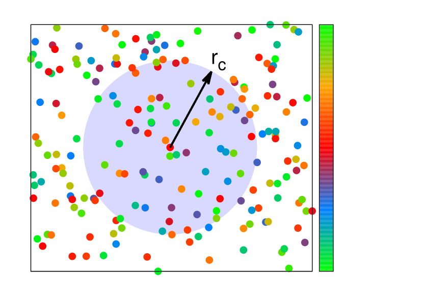
where is the position vector of agent at time in 2-dimensional space with and is the ’s phase angle. Note that the dynamics governed by Eqs. (1) and (2) makes the oscillators swarm and sync. Considering such characteristic we here call the oscillators swarmalators, following the Ref. [3]. is the number of members in the collection composed of such swarmalators whose distances to are not greater than (see Fig. 1). This way, the interaction range of spatial dynamics is bounded by .
is the parameter for attraction with , for which is used in the numerical work below. is the natural frequency of , is a coupling strength of phase and is the total number of swarmalators in system. We consider identical swarmalators with for all in this work.
In the limit, when , Eq. (1) recovers the model suggested in Ref. [2] of special interest in the formation of uniform density and identical radius disc of swarms. The motion of for is basically a gradient flow as each summand can be rewritten by the gradient of a scalar function for . As Eq. (1) with is motivated by the biological aggregations in viscous liquid [21, 25], the inertia effect is ignored to set up an overdamped limit equation [34]. Next when , Eqs. (1) and (2) corresponds to one of the models in Ref. [3], which share common feature of various active and static phases of the swarmalators. Due to the phase variables in Eq. (1), which change in time by Eq. (2), the motion of now has self-propelling property [17, 18, 19]. Equation (2) is a variant of the Kuramoto model [6, 7], i.e., the coupling strength in this prototype model is generalized to in Eq. (2) in order to reflect the spatial configuration in phase dynamics. This was suggested in Ref. [3] to generate pairing current of the swarmalators in a proper range of negative with .
III steady states for infinite cutoff
According to Refs. [2, 3], there are three steady-state patterns when . As we are interested in their reproduction or moderate change for finite , we begin with explaining the three patterns, in a comprehensive way as possible. In the steady states, and for all . Therefore, as its continuum counterpart such as velocity field at position , it is reasonable to set . When one considers a proper coarse-grain of Eq. (1) in the steady states, the velocity field reads
| (3) |
where
| (4) | |||||
with phase field , and is the steady-state density of swarmalators at position with normalization . As Eq. (3) holds for all , it also holds that . Then, in the fact that [35], one finds a self-consistent equation for , which is given by
| (5) |
This self-consistent equation plays a central role in finding the steady-state patterns in the help of other information like symmetry and/or numerical observations.
One of the three steady-state patterns appears when . For positive , Eq. (2) derives the system to phase synchronization state of a common phase . Then, Eq. (1) becomes free from phase as as evolution goes on. In the steady state, therefore, it reads
| (6) |
When this is considered in Eq. (5) in the two-dimensional coordinate, since is constant, using , is immediate. Next, it should be answered where to reside.
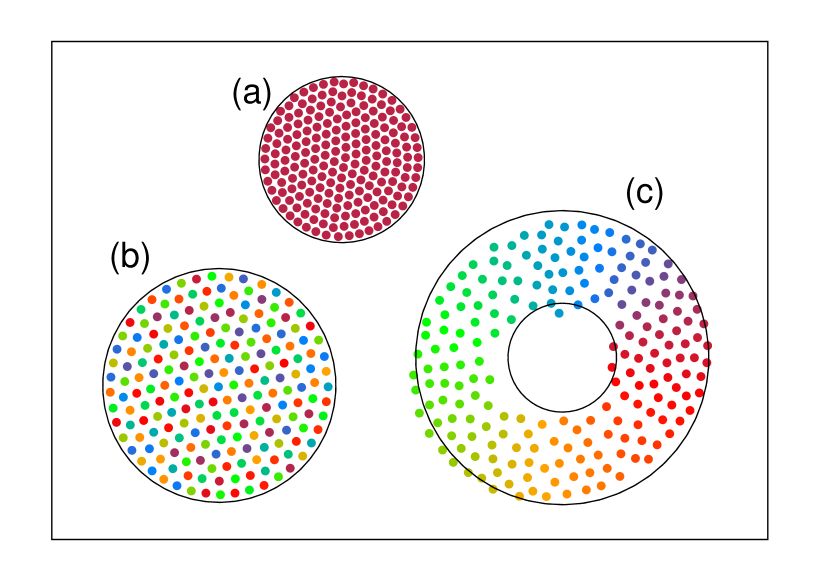
The center of positions is conserved by the symmetric pairs of changes in Eq. (1). Thus when the center is used as the origin, it is natural to expect the rotational symmetry of density, i.e., for . The numerical results always give such distributions that strongly suggest a circular as shown in Fig. 2(a).
Thus when this is considered in Eq. (5), it follows that
| (7) |
where is given by
| (8) |
Interestingly, the density is uniform and the radius depends only on . The pattern by Eqs. (7) and (8) was named the static sync (SS) [3].
The steady-state condition [Eq. (3)] holds for Eq. (7) as follows. When
| (9) |
is introduced, corresponds to Laplace’s equation . Thus, of Eq. (5) gives of the Laplace’s equation, and this is mediated by Eq. (9). As by in Eq. (6) and in Eq. (7), the solution of the Laplace’s equation is given by such cylindrical harmonics of no longitudinal neither angular dependence. Then, the choice should be [35] exclusively or . Here, one excludes the latter as remains finite at in a simple calculation of Eq. (9) with Eqs. (6) and (7). Thus, is immediate for constant .
The second steady-state pattern appears [3] when holds for a negative critical value . For negative , uniform is unstable in Eq. (2), and an erratic profile (asynchrony) would appear. Below , if the configuration of is erratic enough, the summation of the sinusoidal part of Eq. (1) may vanish. When this is the case, reads. This is no more than Eq. (6) with , from which it follows that
| (10) |
This result of uniform density and unit radius successively explains the numerical data shown in Fig. 2(b). This pattern was named the static async (SA) [3].
The third steady-state pattern appears [3] when . For , one trivially reads in Eq. (2). The numerical data shown in Fig. 2(c) indicates can be replaced with the spatial angle of ; for a constant . Then, in polar coordinate , it reads
| (11) | |||||
Using Eq. (11), we find its Laplacian is given by
| (12) | |||||
for proper functions and . Also, the numerically observed circular strip suggests that . Plugging this and Eq. (12) into Eq. (5), one finds
| (13) |
for constant . One again considers Eq. (13) in Eq. (5) to know
| (14) |
Normalization of gives
| (15) |
IV Finite-cutoff of interaction distance
In the numerical study with finite , we have observed various steady-state patterns. Some of them are same as those in the limit, another ones are their proper deformations, and the others are classified as a new class. The three classes appear in order as decreases, and the shape becomes amorphous or non-stationary for further decrease. In the following, the observed patterns are understood and/or described by exploiting Eq. (5), the self-consistent equation for density.
IV.1 SS for
For finite , the system with positive coupling strength is found to be in SS. It is interesting to note that the steady state with multiple discs in SS is discovered (see Fig. 3). Multiple discs of SS have not been found in the system with . Figure 3 is the numerical results of system for when and (we below fix ), displaying the process how the multiple discs of SS are formed.
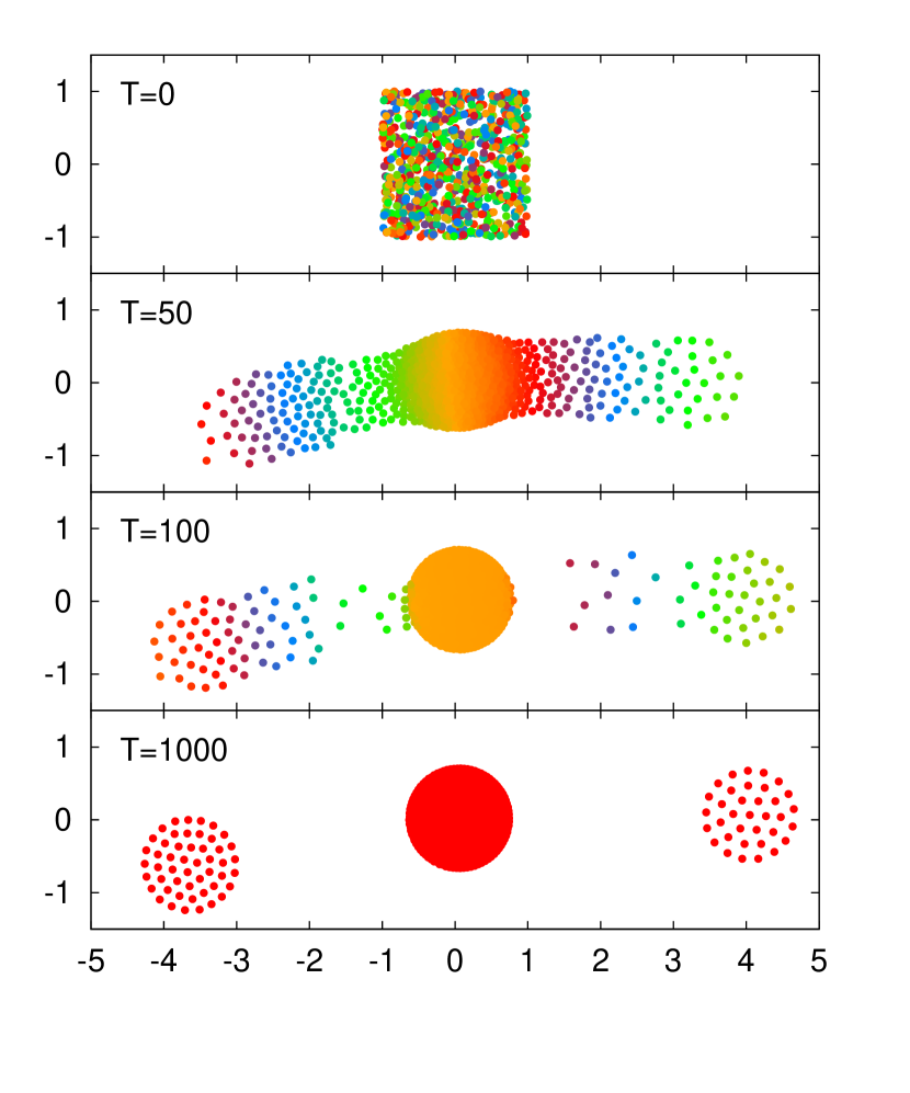
The radius of the discs is, in common, that reminds us of in Eq. (8) with . A simple explanation of this numerical observation is following; the swarmalators are divided into three groups apart from others farther than during transient period, and each group evolves into its own steady state. The snapshots are shown in Fig. 3, from initial via transient to final .
Once a number of swarms is included in a circular region of radius and this region is separated from the others farther than , the dynamics taking place thereafter in the region is identical to that by . If there are several regions separated that way (the number of regions depends on initial condition), the same number of patterns finally appears. We note, when , the self-consistent equation for density [Eq. (5)] does not change from that for . Then, each final pattern becomes no more than the SS of Eqs. (7) and (8). As expected, the discs in the last snapshot are, in common, of radius with their own uniform densities. The minimal separation between the discs is as a consequence of the condition .
With no loss of generality, the condition considered for SS case is generalized to
| (20) |
where is the diameter of a pattern appearing in the limit. It can be SA or SPW beside SS depending on . That is, any of them is expected in the same reason when Eq. (20) holds and, when repeated, the minimal separation is given by the diameter.
IV.2 SA for
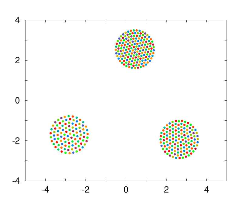
In case of static async, . Thus by Eq. (20), SA should appear for finite when the negatively strong coupling is provided. As expected, the system is found to be in SA where the phases of all the swarmalators are random in the full range of . Also, similar to the previous sync case, the steady state composed of multiple discs of SA is discovered, which has not been found in the system with . Figure 4 shows multiple SA discs for (note for SA).
IV.3 Anomalous SS/SA with nonuniform radial density
Next, we find there appear anomalous steady-state patterns for when , as shown in Fig. 5(a) and (b).
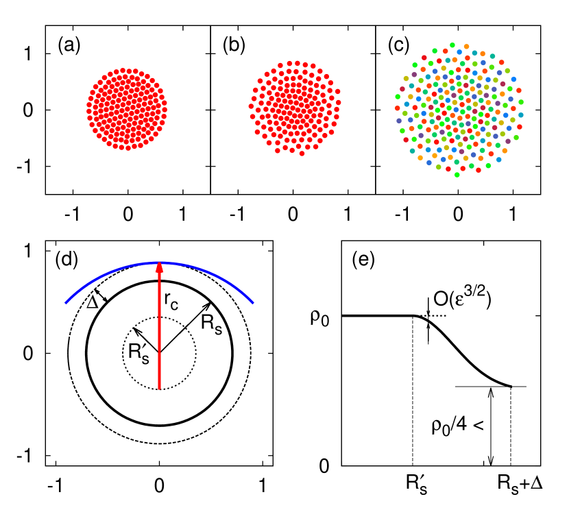
Because Eq. (20) does not hold this time for , what a different pattern may form was in question, and the shown anomalous disc is the result to be understood. The radius becomes larger to . The density looks uniform inside the region of radius while decreases thereafter. These observations can be explained with Eq. (5) as follows.
For finite , it is given from Eq. (6) that
| (21) |
where is the Heaviside step-function assigned with for , or otherwise. Plugging Eq. (21) into Eq. (5) with the numerical observation , one may consider the geometric situations by , , and . Figure 5(d) shows a situation when the interaction range of radius marginally covers the whole distribution of radius ; see the blue arc and the dashed circle tangentially meet. Then, since is constant in the interaction range, Eq. (5) gives . This value does not change as long as the blue circle covers the dashed one, and this is the case when . Note is the very of Eq. (7).
When , the blue circle cannot include the dashed one, and the covered region decreases as increases. So that, in Eq. (5), the integration range becomes smaller for , and this leads to decreasing in the left hand side. Then, one may write
| (22) |
where and is a proper function that decreases for from . Figure 5(e) shows the schematic of Eq. (22). The density begins to decrease from following for small as the area is excluded from the integration in Eq. (5). A lower bound of is simply arguable in the case, which is accompanied with . In this case, when the blue circle is moved to locate its center at , Eq. (5) gives as the integration range covers, at least, a quarter sector of the disc in the dashed circle. Note the coverage is minimized when , so that can be a lower bound of . As the truncated by still shows and the density in Eqs. (21) and (22) also does , follows. Then, a consequent constant gives . Hence, the density in Eq. (22) can be a steady-state configuration. We call this anomalous static sync (aSS).
The aSS explained so far is conditioned in . Meanwhile, the numerical data manifest there should be a lower bound on . For a survey on lower bound, we revisit Fig. 5(d). It states
| (23) |
with and . As is independent of , the lower bound of is reduced to that of . Also in the independence, Eq. (23) shows is decreasing for . Since approaches as decreases, the lower bound of is . Thus when , it reads in the absence of the central constant region. For a simple estimation of , we regard is linear and . From normalization , it follows . Thus considering the above-mentioned upper bound, one finds an interval
| (24) |
for the formation of aSS, and this is, interestingly, consistent with our numerical data. In the other side in (note we set in numerics), we numerically observe the pattern becomes amorphous. is by itself the upper bound of , the radius of aSS. Depending on initial condition, there can appear multiple aSS. After transient period, each region separated farther than from the others has its own disc (not shown here).
Our argument so far is also applicable for the change of the asynchronized-swam disc for while is replaced with . We call the pattern anomalous static async (aSA). An instance is shown in Fig. 5(c). We remark the async-counterpart of Eq. (24), is valid for the smaller criterion than . In the numerical data obtained for , the lower bound shows deviation till (see the upper-left part of the aSA region in Fig. 8). There is more deviation for larger and smaller in the corner. This observation is consistent with the reported stable-region of SA in Ref. [3] for , , in that the criterion is a consequence of linear stability and a smaller means a stronger perturbation. Different from aSS case, aSA does not become amorphous but a non-stationary pattern when it disappears by the decrease of .
IV.4 Variations in SPW
The diameter of SPW that appears when for is . Thus by Eq. (20), for , a formation of the same SPW(s) is expected, and this is numerically observed. Next, for , the results become different, also as expected. However, this time, the difference is not that apparent in shape; the inner and outer radii change a little though the cutoff value is decreased a lot to from . Figure 6(a) is a pattern at , whose inner and outer radii are not discriminated so clearly from and , respectively, known for in Eq. (III).
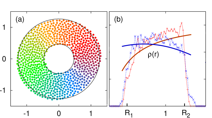
Instead, we have found that a substantial change in density takes place while decreases a lot. In Fig. 6(b), the red pluses come from the numerical data obtained at that is slightly smaller than . Each of them is the count of swarms in a narrow circular region between radii and , where is discrete and small is a few times of the resolution of . Their overall profile is guided by the bold red curve from Eqs. (13), (18), and (III). This guidance is plausible as . The blue crosses in Fig. 6(b) come from the numerical data at , and the blue bold curve is their overall shape as a guide to eyes. The substantial change in density is supposed to compensate for the small change in shape despite the considerable decrease of . We also observed the small change of shape mainly occurs below . The inner and outer radii remain apparently same for while the density change takes place.
A heuristic argument for this observation is following. Let be smaller that , and consider a circle of radius whose center is in somewhere in SPW. If the center is near the outer boundary of SPW, the circle cannot cover the SPW. When this incomplete coverage is considered in Eq. (5), the reduced integral region would lead to density decrease at the center. Next, consider the center is near the inner boundary. In this case, the -radius circle covers the SPW when is provided. For the density of such center, the integral region of Eq. (5) is conserved, and there is no explicit reason to decrease the density. Instead, an opposite reason was already due because the expected density decrease near the outer region requires mass conservation in the system. We consider the cross between the density profiles shown in Fig. 6(b) is the consequence.
If does not hold, the integral region of Eq. (5) is always reduced whatever points of SPW is used for the center of -radius circle. This may indicate a termination of the shape-preserving density change. One then considers an interval
| (25) |
where such SPWs of negligible/considerable change in radius/density for are respectively expected. The lower bound suggested this way is rather comparable with the numerical lower bound in that (see Eq. (III) with for the value). Thus when SPW is specified by the shape only, the condition for its formation is relaxed from to .
We remark that some cases do not give SPW when begins to be smaller than , depending on initial conditions. No appearance of SPW below becomes more frequent for the smaller . Furthermore, SPW does not appear when , at least, numerically. In brief, the numerical data suggests that the basin of attractor [34] for SPW begins to decrease from , and then disappears below .
IV.5 Bar-like patterns at
It is worthy of noting that, when the pattern’s shape is not circular below , it looks linear. According to the numerical data, linear shapes begin to appear for , and disappear when . Figure 7 shows a few linear bar-like patterns (Bar).
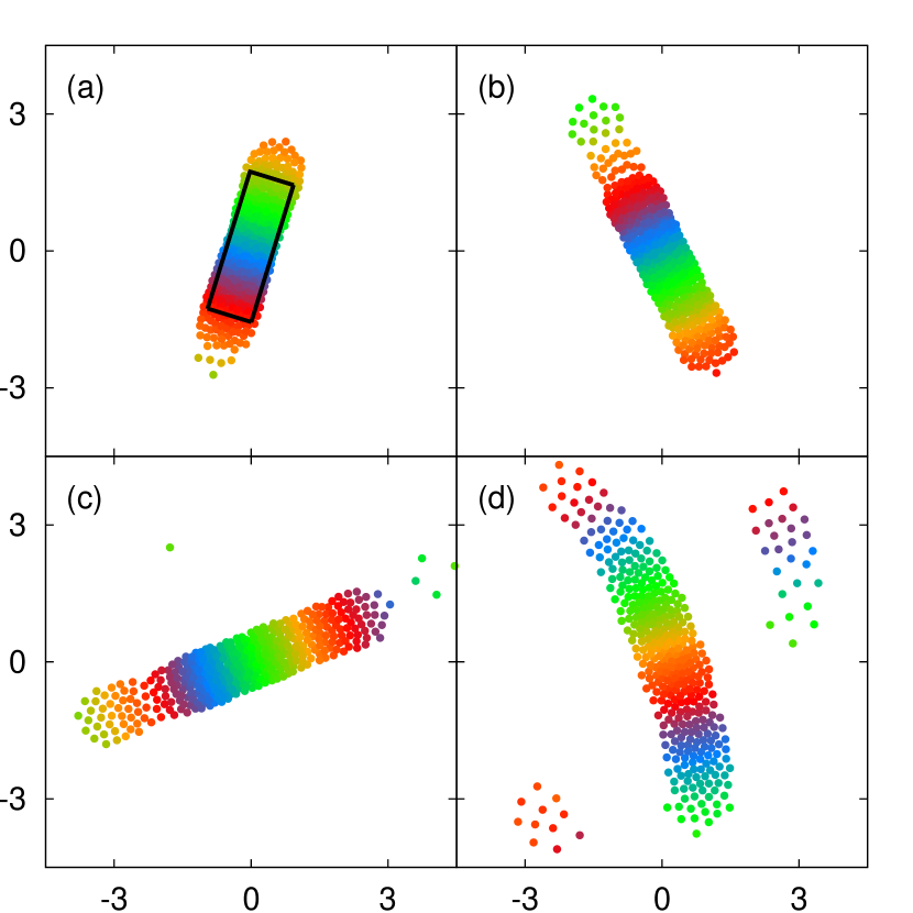
It is inappropriate we consider to view such patterns as the deformed APW by finite . As a first step to the understanding of such bar-like patterns, we below argue that each of them could be a deformed shape, by its own finite , of the bar given as the solution of Eq. (5) in the limit. An ironical situation here is no bar-like pattern has been observed yet in our numerical study neither reported in literature as far as we know. We thus conjecture that a solution bar exists for Eq. (5), of no stability, but it becomes stable for finite accompanied with proper deformation. If our scenario is valid, the pattern of Fig. 7(a) is most close to the solution bar among the figures therein because its is larger than the others’.
We choose -axis as the direction of bar with no loss of generality. In the numerical data, phase smoothly increases along the -axis. The positive direction of the -axis is selected in line with the phase increase. We thus introduce phase field that is differentiable for , and then write
| (26) | |||||
in rectangular coordinate. No dependence on shows Eq. (26) is that for the infinite cutoff.
Consider a bar of length and of width , whose center is the origin. By the symmetry of , we choose for simplicity. We then give a relation between and as
| (27) |
in the consideration of i) s are initialized with uniform random variables in our numerics and ii) any of them does not change in time in Eq. (2) with . By Eq. (27), increases from to , and then remains same thereafter, i.e., for . By differentiabilty, is given. By the symmetry mentioned above, it reads that .
Plugging Eqs. (26) and (27) into Eq. (5), after a little algebra, one can obtain
| (28) |
for and . Obviously, of Eq. (28) is considered for and while elsewhere.
One integrates Eq. (28) to know the area of the solution bar is
| (29) |
Interestingly, the pattern in Fig. 7(a) covers a bar of area by length and width , with a rather tolerable margin (see the guiding black rectangle). This numerical observation suggests and . We also observed the pattern becomes elongated and broadening as decreases. Thus the patterns in Fig. 7(b)-(d) for the smaller also cover the rectangle with the more margins (one can imagine the rectangle in each ones without difficulty). This is consistent with our scenario for the birth of bar-like patterns with finite , proposed above. We also observe in our numerical data that the bar-like pattern is so deformed for that it becomes amorphous.
The rectangle we have specified is a consequence of numerically motivated speculation encapsulated in Eq. (28). This equation is again converted with Eqs. (27) and (29) to
| (30) |
Its solution will lead to the self-consistent equations for and , which can fix the value of and next that of in use of Eq. (29). This way, finding the size of the bar is dual to knowing its density profile. The shooting method looks one of the practical approaches for finding . We leave related interesting task for future work as remarking and is expected with the numerical data up to now.
We add that an 1-dimension result could be relevant to the size of the bar. In 1-dimension, giving is responsible for the repulsion part. Thus when is considered, uniform distribution of width follows. We here consider the swarmalators on -direction segment in the bar are effectively in 1-dimension in that their phases are same so that , the distribution is uniform in the segment as written in Eq. (28), and its width in numerics with is . We leave expected explicit connection between the 1-dimension result and the bar for future work.
The steady-state condition Eq. (3) is a sufficient condition for Eq. (5). That is, the solution of Eq. (5) is not necessarily a steady state. We note of Eq. (28) is not a steady state. For this, one can check the -component of given by cannot balance with its repulsion-counterpart for such that vanishes at (note ). However, with , we observe a steady-state pattern that is rather close to the rectangle expected with Eq. (28), as depicted in Fig. 7(a). We interpret that the bar we speculated with is properly deformed for , and then it becomes stable while still keeping linear shape more or less. The patterns in Fig. 7 are the instances.
V Summary
In this paper, we considered the population of coupled oscillators that sync and swarm under finite-ranged interaction. We explored how the interaction cutoff affects the steady states of the system, with particular attention to the patterns of the steady states. We found that new patterns are induced by the finite-ranged interaction. When the positive/negative phase coupling is present (in the negative case, the coupling below a critical value is considered), multiple clusters forming uniform sync/async discs are found in the static sync/async states. Anomalous discs with nonuniform radial density were also found. In the absence of the phase coupling, APW with abnormal radial density and bar-like patterns of the phase wave state are discovered. We analyzed the new patterns theoretically and numerically to understand their birth and character. The results are summarized in Fig. 8.
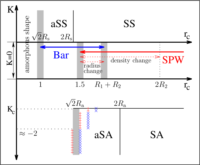
The patterns found for are static in the fact the dynamics becomes a gradient flow in the long time limit. But, it is not trivial whether all the patterns for are stationary because the phase dynamics is frustrated for negative . In this situation, we gave an argument for aSA based on the stability of SA in , reported in Ref. [3]. The lower bound of for aSA, assessed by in our argument, does not reach when , as shown in Fig. 8. The numerical data obtained at the red-cross points near there but still in give completely different patterns that hardly look like instances of aSA. Those are rather comparable with bar-like ones (not shown here). This implies that that part does not belong to aSA but to non-stationary region, on which understanding is out of the scope of this work. A systematic investigation on the left and upper boundary of aSA could be a starting point in studying the non-stationary states by finite . We believe that the steady-state features reported in this work will provide their own starting points in extending the understanding to non-stationary region. Related works will appear elsewhere.
Acknowledgements.
We thank to Agata Barcis and Prof. Christian Bettstetter for useful discussions in the early stage of the study. This study was supported by NRF-2018R1A2B6001790 and 2021R1A2B5B01001951 (H.H), and 2018R1D1A1B07049254 (H.K.L).DATA AVAILABILITY
The data that support the findings of this study are available within the article.
REFERNCES
References
- Bouffanais [2016] R. Bouffanais, Design and Control of Swarm Dynamics (Springer, Singapore, 2016).
- Fetecau, Huang, and Kolokolnikov [2011] R. C. Fetecau, Y. Huang, and T. Kolokolnikov, “Swarm dynamics and equilibria for a nonlocal aggregation model,” Nonlinearity 24, 2681–2716 (2011).
- O’Keeffe, Hong, and Strogatz [2017] K. P. O’Keeffe, H. Hong, and S. H. Strogatz, “Oscillators that sync and swarm,” Nature Comm. 8, 1504 (2017).
- Pikovsky, Rosenblum, and Kurths [2003] A. Pikovsky, M. Rosenblum, and J. Kurths, Synchronization: A universal Concept in Nonlinear Sciences (Cambridge University Press, 2003).
- Winfree [1967] A. T. Winfree, “Biological rhythms and the behavior of populations of coupled oscillators,” J. Theor. Biol. 16, 15–42 (1967).
- Kuramoto [1984] Y. Kuramoto, Chemical Oscillations, Waves, and Turbulence (Springer, Berlin, 1984).
- Kuramoto and Nishikawa [1987] Y. Kuramoto and I. Nishikawa, “Statistical macrodynamics of large dynamical systems. case of a phase transition in oscillator communities,” J. Stat. Phys. 49, 569–605 (1987).
- Crawford [1994] J. D. Crawford, “Amplitude expansions for instabilities in populations of globally-coupled oscillators,” J. Stat. Phys. 74, 1047–1084 (1994).
- Crawford [1995] J. D. Crawford, “Scaling and singularities in the entrainment of globally coupled oscillators,” Phys. Rev. Lett. 74, 4341–4344 (1995).
- Crawford and Davies [1999] J. D. Crawford and K. T. R. Davies, “Synchronization of globally coupled phase oscillators: singularities and scaling for general couplings,” Physica D 125, 1–46 (1999).
- Strogatz [2000] S. H. Strogatz, “From kuramoto to crawford: exploring the onset of synchronization in populations of coupled oscillators,” Physica D 143, 1–20 (2000).
- Acebron et al. [2005] J. A. Acebron, L. L. Bonilla, C. J. P. Vicente, F. Ritort, and R. Spigler, “The kuramoto model: A simple paradigm for synchronization phenomena,” Rev. Mod. Phys. 77, 137–185 (2005).
- Hong, Park, and Choi [2005] H. Hong, H. Park, and M. Y. Choi, “Collective synchronization in spatially extended systems of coupled oscillators with random frequencies,” Phys. Rev. E 72, 036217 (2005).
- Hong et al. [2007] H. Hong, H. Chate, H. Park, and L.-H. Tang, “Entrainment transition in populations of random frequency oscillators,” Phys. Rev. Lett. 99, 184101 (2007).
- Hong and Strogatz [2011] H. Hong and S. H. Strogatz, “Kuramoto model of coupled oscillators with positive and negative coupling parameters: An example of conformist and contrarian oscillators,” Phys. Rev. Lett. 106, 054102 (2011).
- Partridge [1982] B. L. Partridge, “The structure and function of fish schools,” Scientific American 246, 114–123 (1982).
- Reynolds [1987] C. W. Reynolds, “Flocks, herds, and schools: A distributed behavioral model,” Computer Graphics 21, 25–34 (1987).
- Vicsek et al. [1995] T. Vicsek, A. Czirok, E. Ben-Jacob, and I. Cohen, “Novel type of phase transition in a system of self-driven particles,” Phys. Rev. Lett. 75, 1226–1229 (1995).
- O’Loan and Evans [1998] O. J. O’Loan and M. R. Evans, “Alternating steady state in one-dimensional flocking,” J. Phys. A: Math. Gen. 32, L99–L105 (1998).
- Czirok, Barabasi, and Vicsek [1999] A. Czirok, A.-L. Barabasi, and T. Vicsek, “Collective motion of self-propelled particles: kinetic phase transition in one dimension,” Phys. Rev. Lett. 82, 209–212 (1999).
- Mogilner and Edelstein-Keshet [1999] A. Mogilner and L. Edelstein-Keshet, “A non-local model for a swarm,” J. Math. Biol. 38, 534–570 (1999).
- Rauch, Millonas, and Chialvo [1995] E. Rauch, M. Millonas, and D. Chialvo, “Pattern formation and functionality in swarm models,” Phys. Lett. A 207, 185–193 (1995).
- Hubbard et al. [2004] S. Hubbard, P. Babak, S. T. Sigurdsson, and K. G. Magnússon, “A model of the formation of fish schools and migrations of fish,” Ecol. Model. 174, 359–374 (2004).
- Lee et al. [2004] H. K. Lee, R. Barlovic, M. Schreckenberg, and D. Kim, “Mechanical restriction versus human overreaction triggering congested traffic states,” Phys. Rev. Lett. 92, 238702 (2004).
- Topaz, Bertozzi, and Lewis [2006] C. M. Topaz, A. L. Bertozzi, and M. A. Lewis, “A nonlocal continuum model for biological aggregation,” Bull. Math. Bio. 68, 1601–1623 (2006).
- O’Keeffe, Evers, and Kolokolnikov [2018] K. P. O’Keeffe, J. H. M. Evers, and T. Kolokolnikov, “Ring states in swarmalator systems,” Phys. Rev. E 98, 022203 (2018).
- O’Keeffe and Bettstetter [2019] K. O’Keeffe and C. Bettstetter, “A review of swarmalators and their potential in bio-inspired computing,” in Proc. SPIE 10982, Micro- and Nanotechnology Sensors, Systems, and Applications XI (2019) p. 10982.
- Ha et al. [2019] S.-Y. Ha, J. Jung, J. Kim, J. Park, and X. Zhang, “Emergent behaviors of the swarmalator model for position-phase aggregation,” Mathematical Models and Methods in Applied Sciences 29, 2271–2320 (2019).
- Barciś, Barciś, and Bettstetter [2019] A. Barciś, M. Barciś, and C. Bettstetter, “Robots that sync and swarm: A proof of concept in ros 2,” (IEEE, 2019).
- Baris and Bettstetter [2020] A. Baris and C. Bettstetter, “Sandsbots: Robots that sync and swarm,” IEEE Access 8, 218752–218764 (2020).
- McLennan-Smith, Roberts, and Sidhu [2020] T. A. McLennan-Smith, D. O. Roberts, and H. S. Sidhu, “Oscillatory behavior in a system of swarmalators with a short-range repulsive interaction,” Phys. Rev. E 102, 032607 (2020).
- Lizarraga and de Aguiar [2020] J. U. F. Lizarraga and M. A. M. de Aguiar, “Synchronization and spatial patterns in forced swarmalators,” Chaos 30, 053112 (2020).
- Jiménez-Morales [2020] F. Jiménez-Morales, “Oscillatory behavior in a system of swarmalators with a short-range repulsive interaction,” Phys. Rev. E 101, 062202 (2020).
- Strogatz [1994] S. H. Strogatz, Nonlinear Dynamics and Chaos (Addison-Wesley, MA, 1994).
- Arfken and Weber [2005] G. B. Arfken and H. J. Weber, Mathematical Methods for Physicists, 6th ed. (Elsevier, Amsterdam, 2005).