Collective excitations in magnetic topological insulators and axion dark matter search
Abstract
We investigate collective excitations in magnetic topological insulators (TIs) and their impact on axion detection. In the three-dimensional TI model with the Hubbard term, the effective action of magnons and amplitude modes is formulated by dynamical susceptibility under the antiferromagnetic and ferromagnetic states. One of the amplitude modes is identified as “axionic” quasi-particle and its effective coupling to the electromagnetic fields turns out to be enhanced by about four orders of magnitude larger than the previous estimate, which may drastically change the sensitivity of the axion search using “axion” in magnetic TIs.
1 Introduction
Axion and axion-like particles are candidates for dark matter of the universe Preskill:1982cy ; Abbott:1982af ; Dine:1982ah . While many observations have been dedicated to the search, it is yet to be found so far. Recently, the dynamical ‘axion’, as a quasi-particle in condensed matter, has drawn attention in the context of the axion dark matter search. The ‘axion’ couples to the electromagnetic field and Ref. Marsh:2018dlj proposed an axion search in the mass range of meV using the magnetic topological insulators (TIs).111See, for examples, Refs. Tokura2019 ; Bernevig2022 ; Liu2023 ; Sekine_2021 , for recent reviews of magnetic TIs.
The mass scale is based on an estimation of the mass of the dynamical ‘axion’ in the TIs Li:2009tca . Bi2Se3, Bi2Te3, and Sb2Se3 are the representative examples of three-dimensional (3D) TIs. Since the TIs do not have magnetic order, it is assumed in this estimation that magnetic impurities, such as Fe or Cr, are doped to Bi2Se3 so that the materials have ferromagnetism (FM) or antiferromagnetism (AFM). Then Ref. Li:2009tca proposes that the magnetism is described by introducing the Hubbard interaction term. Namely, the total model consists of the effective Hamiltonian for the 3D TIs and the Hubbard term. In the literature the ‘axion’ mass is estimated to be about 1 meV. On the other hand, it was shown in Ref. Ishiwata:2021qgd that the typical mass of the ‘axion’ is of the order of eV, independent of the topology of insulators, in the same model. The study also indicates that it can be suppressed near the phase boundary of the AFM order. Similar results are reported in a different model in which the spin interaction term between the magnetic impurity and electron is introduced Ishiwata:2022mzq . In the study the phase transitions of the AFM and FM are shown and the ‘axion’ mass is typically eV in both phases.
Determination of the ‘axion’ mass is crucial for the proposed axion search. Furthermore, it is important to find a magnetic environment that is suitable for the axion detection. In fact, the first-principles calculation shows that Mn2Bi2Te5, which is recently synthesized experimentally PhysRevB.104.054421 , has a variety of magnetic states Li:2020fvr . In the literature the topological phases are tuned by layer magnetization and the energy gap is computed in each magnetic state. Tuning of magnetism by an electric field in magnetically doped TIs is discussed in Ref. Wang_2015 . On the other hand, Ref. Lhachemi:2023eha claims that magnetic field induces an effective phonon charge, which plays a role of ‘axion.’ These studies inspire us to search for other possible magnetic excitations that may be utilized for the axion search.
In this paper, we investigate possible collective excitations in the magnetic TI model and study their impact on the axion detection. To this end, we revisit the original model of the magnetic TIs, i.e., the effective model for 3D TIs augmented by the Hubbard term. Starting from the partition function, the effective action for the excitations is derived using the dynamical susceptibility. The emergence of the AFM and FM orders is shown and we analyze the gap and dispersion relation of eight magnetic excitations that consist of the amplitude modes and magnons with various types.222The amplitude mode is also called ‘Higgs amplitude mode’ and various experimental efforts have been made to detect it, for instance, in low-dimensional magnetic materials PhysRevLett.85.832 ; PhysRevLett.89.197205 ; PhysRevLett.93.257201 ; PhysRevLett.100.205701 ; Jain_2017 ; Hong_2017 or frustrated magnetic materials PhysRevB.97.140405 ; osti_1571849 . For the theory of the spin wave, see, for example, Refs. PhysRev.81.869 ; PhysRev.85.1003 ; PhysRev.87.60 ; PhysRevB.64.184423 ; PhysRevB.93.094438 . We identify one of the amplitude modes as ‘axion’ and one of the magnons also can play the role of ‘axion’ in a specific case. The validity of the effective description of the excitations is clarified and some excitations are found to be unstable.
The paper is organized as follows. The effective action is derived from the model in Sec. 2. From the effective action the effective potential for the order parameters of the AFM and FM is calculated in Sec. 3, and the features of the magnetic orders are discussed. In Sec. 4 the effective actions of the eight types of collective excitations are derived and the dispersion relation and the stability of the excitations are described. Here we identify the ‘axion’ quasi-particle and investigate its properties. Based on the results, we discuss a direction to realistic axion search in Sec. 5. Sec. 6 is devoted to conclusion.
In our study, we adopt natural units where .
2 The model
To discuss possible magnetic orders, we consider an effective Hamiltonian for 3D TIs Zhang:2009zzf ; Li:2009tca ; Liu_2010 that is augmented by the Hubbard term. The Hamiltonian of the model is given by
| (1) |
where
| (2) | ||||
| (3) |
Here is a positive constant, and are the indices of the sublattice and site, respectively. is the number density of the electrons at the site with spin and . will be given later. In our study, we consider axis as the easy axis. By the Stratonovich-Hubbard transformation, the Hubbard term is written by introducing two fields :
| (4) | ||||
| (5) |
where and are 4 by 4 matrices defined as
Here are the Pauli matrices. Appendix A.1 gives the list of the Gamma matrices that are used in this study. is physically the spin moment in direction at site of sublattice and we have introduced
| (6) | |||
| (7) |
When and are constants, then their constant values correspond to the order parameters of the AFM and FM, respectively. The term proportional to is considered in Refs. Rosenberg_2012 ; Kurebayashi_2014 ; Wang:2015hhf in different models. Then (Euclidean) action is given by
| (8) |
where is the imaginary time and
| (9) |
is the inverse temperature. The effective action is given by integrating out the electron field in the partition function , i.e.,
| (10) |
which leads to
| (11) |
We will use and to derive the effective potential for the order parameters in the next section.
3 Magnetic orders
In this section we find possible global orders of the magnetism and identify the ground state. For this purpose, we ignore the local quantum fluctuations and compute the effective potential following the technique of Ref. Ishiwata:2022mzq .
3.1 The effective potential
The effective potential is derived from the grand potential. The grand potential is defined by the partition function :333Though we give the formulae with finite temperature, we will focus on the zero temperature limit in the later numerical study.
| (12) |
The effective potential per site is then obtained by taking and as constants, i.e., and ,
| (13) |
where is the number of the cite, is the chemical potential, is the band index, and is the wavenumber. will be given soon. In the derivation, we have adopted the Matsubara formalism, which gives
| (14) |
where is the Matsubara frequency for fermion. are the eigenvalues of , which is in the wavenumber space:
| (15) |
where
| (16) | ||||
| (17) |
( - 4) are the Gamma matrices given by
and we take without loss of generality. is a constant and is parametrized as Zhang:2009zzf ; Li:2009tca ; Liu_2010
| (18) |
where . In the following study, we consider a cubic lattice and use dimensionless wavenumber for simplicity, i.e., . The first and second terms of have the time-reversal invariance, which is one of the features of the TIs, and it describes Bi2Se3 family of materials. The eigenvalues are obtained as , where
| (19) | ||||
| (20) |
Here and . Since we focus on the insulated states, we consider that the electrons are half-filled. Namely, we take and two lower bands and are filled.
For later analysis, we derive the stationary conditions for the possible magnetic orders. For the AFM, it is given by , and the result is
| (21) |
where is a nonzero stationary value, and is the Fermi-Dirac distribution function. Similarly, gives a nonzero that satisfies
| (22) |
For both the AFM and FM cases, it is easy to check that as , which corresponds to a case where the magnetism is saturated.
Before computing the effective potential, we discuss conditions for the AFM and FM orders. To this end we take limit, which leads to
| (23) |
Regarding the AFM, we expand the effective potential up to while taking to obtain
| (24) |
Therefore we expect to have the AFM order when
| (25) |
Similarly, one may get a condition to have the FM order as
| (26) |
However, it is not an exact condition for the FM order; the FM order may arise even when (26) is not satisfied. This can be understood by expanding the effective potential at :
| (27) |
The coefficient of a term proportional to can be negative, which may lead to the FM order. We will confirm this numerically later. Even though it is not an exact condition, (26) can be used to understand the qualitative behavior of the emergence of the magnetic order. I.e., we expect that the FM order will appear for relatively larger and than and , in other words, larger compared to , , , and .
On the other hand, if is exactly satisfied, the effective potential becomes
| (28) |
Thus, the FM order appears without other conditions, and the stationary point is given by . We will discuss this specific case later.
Both conditions (25) and (26) are satisfied in the limit . Thus, the AFM and FM order should appear in the large limit.
3.2 Numerical results
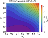
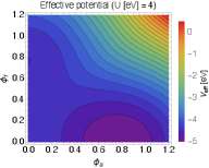
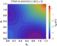
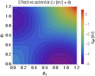
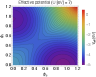
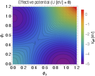
Now we are ready to show the effective potential on plane. Fig. 1 shows the effective potential for a given set of parameters. We take and the normal insulator (NI) phase is considered. The TI phase can be calculated by taking with the others being unchanged and we found the result merely changes. It is seen the potential minima appear as increases. As gets large, the AFM order forms first since the condition for the AFM order, i.e., (25), is relatively easy to satisfy, and eventually the FM order shows up.
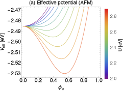
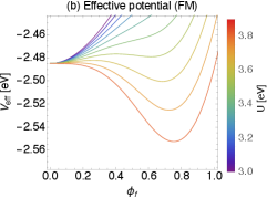
To see the emergence of the magnetic orders, Fig. 2 shows the effective potential as function or . It should be noted that appears continuously from zero meanwhile the non-zero is obtained discontinuously. For the FM order, it is seen that another vacuum appears as the becomes larger while the coefficient of the quadratic term is positive. This is due to the negative term in Eq. (27). Such a situation never happens for the AFM since the quartic term is always positive. In fact, the phase transition to the AFM order happens when the value of exceeds a critical value defined by
| (29) |
In the present parameter set, i.e., eV, eV, and eV, we find eV.
Regarding to the ground state of the magnetic order, we have numerically checked that the minimum of the effective potential is obtained when the magnetic state is the AFM. This is true for other sets of parameters. Therefore, the ground state of the system is the AFM order. On the other hand, both minima for the AFM and FM orders get degenerate as . This can be understood analytically. In the large limit, the stationary points reduce to and and , . Thus both minima approach to
| (30) |
Therefore, when the magnetization is saturated, i.e., , both AFM and FM orders are expected to be realized as quasi-degenerate vacua.
To summarize, we have seen the emergence of the AFM and FM orders by computing the effective potential from the grand potential and found that the AFM is the ground state. On the other hand, the AFM and FM states are degenerate as gets larger.
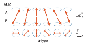
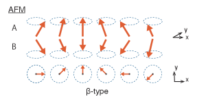
4 The amplitude mode and magnon under magnetic order
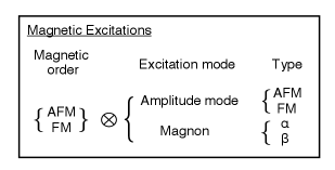
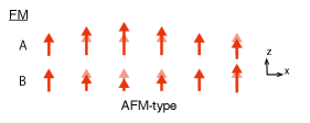
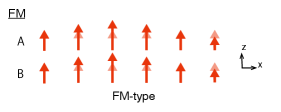
In this section, we evaluate the gap and dispersion relation of the magnetic excitations under the magnetic orders. As seen in the previous section, the possible magnetic orders are the AFM and FM and the former is the ground state. To consider the excitations under both magnetic environments, we take or , where and are constants that satisfy Eqs. (21) and (22), respectively. We will see that there are two magnetic excitations, that are amplitude mode and magnon, and each of them has two types. Fig. 3 (left panel) shows the classification of the excitations. We will also discuss an excitation called ‘axion’ in the magnetic TIs.
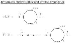
4.1 Dynamical susceptibility and inverse propagator
For the study we introduce a dynamical susceptibility, which is defined by
| (31) |
where is the Green’s function of the electron under the global magnetic order, AFM or FM, in the wavenumber space, which will be defined soon. The index and stands for the magnetic order, i.e., AFM and FM, respectively. and are four by four matrices, such as Gamma matrices. For the arguments of the susceptibility and the Green’s function, we write and as and . Instead of , we will use a dynamical susceptibility that is symmetric with respect to and :
| (32) |
Here is a label for a specific set of operators and , which will be given explicitly in this section.
With the dynamical susceptibility, we will see that defined by
| (33) |
plays the role of the inverse propagator, which is normalized to be dimensionless, of the excitations at the one-loop level. Fig. 3 (right panel) shows diagrams that correspond to the dynamical susceptibility and the inverse propagator .
4.2 The amplitude mode
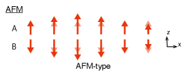
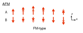
To discuss the amplitude mode, we take
| (34) | ||||
| (35) |
and are two independent fluctuations of the AFM and FM order parameters, respectively, and we call them ‘AFM-type’ and ‘FM-type.’ The example of the fluctuations are shown in Fig. 4. One can imagine that there are four excitations by looking at the effective potential in Fig. 1; the AFM- and FM-type amplitude modes under the AFM correspond to the fluctuations around in and directions, respectively, and a similar interpretation applies to the fluctuations around . From the figure we naively expect all the amplitude modes to be stable. This intuition, however, needs to be modified, which will be discussed below.
With Eqs. (34) and (35), we expand the second term of Eq. (11) as444Similar expansion is done in Refs. Sekine:2015eaa ; Sekine_2021 ; Schutte-Engel:2021bqm to derive ‘axion’ mass, meanwhile the first term of Eq. (5), i.e., that will give rise to a term in Eq. (39), is missing at the beginning. When this term is missing, then the resultant ‘mass term’ gets the opposite sign, leading to the tachyonic instability. The authors, however, claim that they obtain the same result as one in Ref. Li:2009tca though their calculation is inconsistent. See also discussion below Eq. (45).
| (36) |
by decomposing where
| (37) | ||||
| (38) |
Then the Green’s function is given by where and for and , respectively. Using the definition of the Fourier expansion of the field and the Green’s function given in Appendix A.2, the effective action at is
| (39) | ||||
| (40) |
where is given in Eq. (33) and
| (41) | ||||
| (42) |
The first term of comes from the first term in Eq. (39), which is the tree-level contribution mass term and the second one corresponds to the loop diagram. plays a role of an inverse propagator of the excitations at the one-loop level while it is normalized to dimensionless in our notation. Thus plays a role of the connected two-point Green’s function that is given by summing over the infinite series of the one-loop diagram. can be evaluated in the basis where the Green’s functions are diagonalized. The calculation is shown in Appendix B. From Eq. (40), the gap and dispersion relation of the amplitude mode is given by solving
| (43) |
where .
Before the numerical study, we comment on the ‘axionic’ excitation in the magnetic TIs. We claim that the AFM-type amplitude mode under the AFM order corresponds to the quasi-particle ‘axion,’ regardless of the topological nature of the insulators. Namely, the ‘axion’ corresponds to the AFM-type amplitude mode in both TI and NI phases.555The existence of the dynamical ‘axion’ in NIs with the AFM state is already pointed out in Ref. Ooguri:2011aa . The dynamical ‘axion’ is also studied under the FM order in Ref. Wang:2015hhf ; Ishiwata:2022mzq . First of all, the gap of the AFM-type amplitude mode under the AFM order, obtained by Eq. (43), corresponds to the mass of the ‘axion’. This fact is understood from the fact that is the inverse propagator of the excitation and that the pole of the propagator gives the physical mass. To derive the effective action for the ‘axion,’ let us take the zero temperature limit. First, the mass of ‘axion’ is given by
| (44) |
It is easy to find a solution for the equation by using an analytic expression for given Eq. (105) of Appendix C:
| (45) |
for .666The ‘axion’ mass can be obtained by solving numerically for case. Then, expanding at and and taking a continuum limit for the space, we get the action of the ‘axion’ in the Minkowski spacetime as
| (46) |
where an index is summed from 1 to 3 and
| (47) |
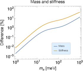
Here and are the stiffness and velocity, respectively. See Appendix D for the derivation of the action. The results of the mass and stiffness given in Eqs. (45) and (47) are different from the previous results Ishiwata:2021qgd 777 and in Refs. Li:2009tca ; Schutte-Engel:2021bqm ; Sekine:2015eaa ; Sekine_2021 are smaller than those in Ref. Ishiwata:2021qgd by a factor of 4, which was already pointed out in Ref. Ishiwata:2021qgd .
| (48) | ||||
| (49) |
The reason is that the previous results are given by expanding at , not . This is based on the assumption that the expansion around is a good approximation. However, the quantitative argument regarding the validity of the expansion around has not been clarified explicitly in the previous works.
Compared to the previous calculation, we have two improvements. First, the mass and stiffness given in the present work are more accurate. This is because we do not use perturbative expansion to derive the mass and that the stiffness is derived by the derivative of with respect to at the mass. Second, it is possible to check whether the gap (or mass) obtained at is the minimum. Namely, there is a possibility that a smaller gap is obtained for a nonzero . In such a case, we must expand at the wavenumber to derive the effective action for the lower-energy excitation. We will check this possibility numerically below.
By the use of the effective action, we can evaluate the validity condition of the perturbative expansion of the past works. As a result, we found that the expansion is valid for . The details are given in Appendix D.
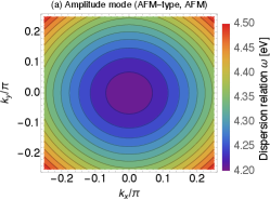
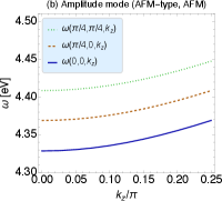
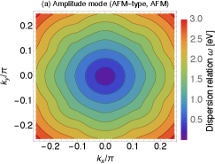
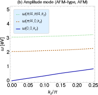
Fig. 5 shows the dispersion relation of the AFM-type amplitude mode under the AFM order. We take and the other parameters are the same as Fig. 1. We found that is the stable minimum. Here ‘stable’ means that the curvature of the dispersion relation is positive in all directions around . In other word, are positive for all – 3. This can be seen explicitly in the figure. We have checked that there are no smaller gaps, thus the gap is surely given by .
The situation is different for the other amplitude modes. As an example, let us discuss the FM-type amplitude mode with the AFM order. The dynamical susceptibility of the excitation is analytically obtained by (see Appendix C)
| (50) |
where and – depend on the wavenumber as , , , and . When , for instance, we found that the gap is found to satisfy , where . In addition, the imaginary part of is enhanced. This indicates that the amplitude mode tends to dissipate to an electron-hole pair. One can understand the interpretation of the imaginary part from a corresponding diagram to the dynamical susceptibility, shown in Fig. 3. Similar behavior is found for nonzero . Therefore, the excitation is not stable and dissipates even if it is created. We have also found no stable configuration for both AFM- and FM-type amplitude modes under the FM order. In addition, the expansion for is inappropriate since can be larger than unity. Therefore, the effective description of the form of Eq. (46) is invalid for those excitations.
4.3 The magnon
To describe the magnon, we need to rewrite the Hubbard term in an isotropic form. Namely, the Stratonovich-Hubbard transformation gives
| (51) |
where that satisfies . Under the AFM, , while for the FM. Recalling that we are interested in the case where direction is the easy axis, the fluctuation of corresponds to the magnon. For later analysis we introduce and as
| (52) | |||
| (53) |
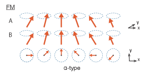
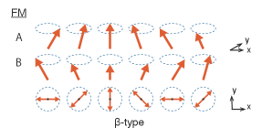
The labels and stand for two different types of magnon excitations, which we call ‘-type’ and ‘-type,’ respectively. We will formulate each excitation under both the AFM and FM orders below.
First, let us discuss the magnon under the AFM order. and are parallel for the -type, meanwhile rotation phases of and coincide for the -type. See Fig. 6 (top panel) for an example of the - and -types under the AFM. The interaction Hamiltonian gives
| (54) |
where
Assuming that the Hamiltonian reduces to where
| (55) |
The term proportional to does not contribute to AFM order and we will ignore it hereafter. Now it is convenient to introduce
| (56) | |||
| (57) |
Using them, is written as
| (58) |
where
Now we derive the effective action in a similar way as in Sec. 4.2. Computing the terms up to , the effective action for the excitations is
| (59) |
where is given in Eq. (33) and () are given by
| (60) | ||||
| (61) |
Here the first term of is given by the term proportional to in Eq. (58). Diagrammatically it is a tadpole and we have found that it can be rewritten by using Eq. (21). As a result, it turns out to have the same structure as the amplitude modes.
We repeat the argument for the FM order. In this case, we take to give the Hamiltonian
| (62) |
As seen, the Hamiltonian is given by a replacement , , , and in Eq. (54). Then the perturbative term in the Hamiltonian becomes,
| (63) |
Here we have omitted a term proportional to that is ineffective for the FM order. The effective action is then obtained by
| (64) |
and
| (65) | ||||
| (66) |
The first term of comes from the term proportional to . It corresponds to the tadpole diagram and it can be rewritten by using Eq. (22). Thus the structure is the same as . With the FM order, the -type and -type of magnon corresponds to and , respectively, which are shown in Fig. 6 (bottom).
From the expressions of the effective action regarding magnons, i.e., Eqs. (59) and (64), the gap and dispersion relation of the magnon is given by
| (67) |
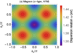
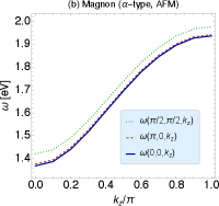
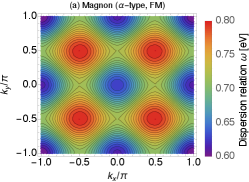
Now we show the numerical results of the dispersion relation of the magnons. Fig. 7 shows a plot of the dispersion relation regarding the -type magnon under the AFM order. We have found the dispersion relation is minimized at . On the other hand, there are additional quasi-degenerate values of at . The degeneracy is about 1%, compared to and the curvatures of the wavenumbers are positive at the s. Therefore we expect four different stable configurations of the magnon. The excitation energy is found to be around eV.888When we derive the effective action for those configurations of magnon, we need to expand around each wavenumber, i.e., .
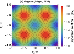
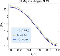
Fig. 8 shows the dispersion relation for the -type magnon under the AFM order. For the excitation similar result to the -type is obtained but with a different configurations; we have found has the minimum at , and cross values are found at with a degeneracy of around 1%. The energy scale turns out to be the same as the -type one, i.e., .
It is worth discussing the origin of the gap of the magnons. Let us consider the -type magnon under the AFM at zero temperature. Assuming that the expansion around is valid, we get the stiffness and mass of the magnon as (see Appendix D for the derivation)
| (68) | ||||
| (69) |
It is clear that magnon is gapped at the zero temperature. From the expression, we see that gap is typically , which is consistent with the numerical result shown in Fig. 7. The typical scale is the same as the AFM-type amplitude mode under the AFM. However, the parameter dependence is different; in the limit, and leads to . Therefore, the gap remains to be even if is much larger. We have also confirmed this numerically.
Based on the above argument, we expect that the gap of the magnon becomes zero when . This can be confirmed without the expansion with respect to ; considering the zero wavenumber and taking the limit at the zero temperature, Eq. (67) with and gives rise to
| (70) |
Recalling Eq. (21), it is easy to find is the solution to satisfy the gap equation. Therefore nonzero and (or ) are the origin of the -type magnon gap under the AFM. This can be understood by considering the symmetry breaking of the system. When , SO(3) symmetry in the space is restored. Under the AFM order, the nonzero breaks the SO(3) to SO(2). Consequently two massless Nambu-Goldstone bosons appear, which correspond to . See Appendix E for more detail.
Since we already have identified Nambu-Goldstone bosons, another excitation, -type magnon under the AFM order, should be massive even if . In fact, by expanding around , the stiffness and mass are given by
| (71) | ||||
| (72) |
Thus a finite mass (or gap) should appear even if .
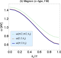
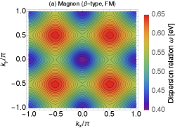
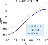
The results for -type and -type magnons under the FM state are similarly computed. It is found that qualitative features of the -type and -type ones are the same as the - and -types under the AFM order, respectively. Typical energy scale of the excitations are a bit smaller but they are . See their plots in Appendix F.
To summarize this section, we have formulated the effective actions of the amplitude modes and magnons under both the AFM and FM orders. Each mode has two types; the amplitude mode has AFM- and FM-types and the magnon has the - and -types. From the effective action, we have computed the dispersion relations for all excitations. Among them, the AFM-type amplitude mode is identified as the ‘axionic’ quasi-particle. We have found that the mass of ‘axion’ coincides with the gap and it is derived more precisely compared to the past works. The typical energy scale turns out to be eV and the other excitations have the same scale.
5 Implication to axion search
As seen in Sec. 4.2, the ‘axionic’ excitation corresponds to the AFM-type amplitude mode (up to normalization of the field) under the AFM, and it is shown its mass (or gap) is given by . On the other hand, the energy bands of the electrons of the magnetic TIs are computed by the first-principles calculation. For , as an example, Ref. Li:2020fvr shows that the gap of the electrons under the AFM order is meV. With this knowledge, we discuss the possibility of the axion detection by using the interaction of the ‘axion’ with the electromagnetic fields.
The ‘axion’ field has an coupling in the Lagrangian Li:2009tca :
| (73) |
where is the fine-structure constant and is the field strength of the electromagnetism.999 are the Lorentz indices that are 0, 1, 2, 3. is the dual of , defined as ( is the Levi-Civita symbol with ) and is related to the model parameters of the 3D TIs as Li:2009tca
| (74) |
with being 1, 2, 3, and 5.
Recalling that the effective action for the AFM-type amplitude mode under the AFM is given in Eq. (46), we define a canonically normalized field :
| (75) |
Therefore, using
| (76) |
the interaction term can be written in a form,
| (77) |
where
| (78) |
Therefore, works as an effective“decay constant” for axion.101010Be aware that there is an additional factor of in the coupling. In terms of a variable (or in our notation) in the literature Li:2009tca ; Zhang_2020 , it is given by
| (79) |
Or it is equivalent to used in Ref. Marsh:2018dlj , i.e.,
| (80) |
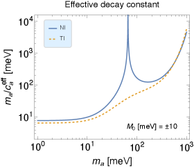
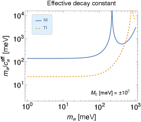
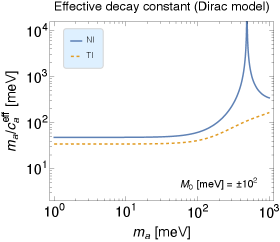
We plot the effective decay constant of the amplitude mode as function of in Fig. 9. Here we have used the fact that the AFM order parameter becomes nonzero continuously as increases shown in Sec. 3. Therefore can take any value from zero to if the value of is properly chosen. In the plot the results for the NI and TI phases are given by taking meV for comparison. Here we note that the enhancement point corresponds to a root of . While the results of the NI and TI are similar for meV, those with meV are different. This quantitative difference comes from the 3D TI model, which will be discussed below. To put it simply, we found that the effective coupling is meV for 100 meV.
Ref. Marsh:2018dlj , which proposes the axion detection using ‘axion’ in the magnetic TIs, claims that the effective decay constant is about eV, based on Ref. Li:2009tca . However, this is larger than our result by . Let us see this more closely. In Ref. Li:2009tca , they use a variable ,111111We have changed the expression in the literature to one in the natural unit. where T and , and estimate as meV. Using this relation, can be calculated as eV, which is close to the value given in Ref. Marsh:2018dlj . Namely, the estimate of meV in Ref. Li:2009tca indicates eV. One may think that this discrepancy comes from another choice of the input parameters. However, such a possibility is unlikely from an analytic estimation below.
Let us focus on the case where meV that is considered in Ref. Li:2009tca . To take an analytic approach, we consider the Dirac model instead of the 3D TI model. The Dirac model is given by expanding the 3D TI model around . See Eq. (133) for the explicit form. It is empirically known that physical properties of the excitation near its gap are unchanged in either model. Thus, the Dirac model can be a good tool to understand the physical behavior analytically. Since this scale is much smaller than the energy scale of the electrons, in the Dirac model is approximately given by Ishiwata:2021qgd
| (81) |
which leads to
| (82) |
In addition, is estimated as
| (83) |
The estimation above is also checked numerically. Therefore, we get
| (84) |
for . This estimation is roughly consistent with the results shown in Fig. 9. For a reference, we have computed the effective decay constant with the Dirac model. See Appendix F for the plots of the results. We note that does not exceed the typical energy scale of the electron, i.e., . This is the reason that the value is unlikely.121212Ref. Schutte-Engel:2021bqm indicates 30 eV, which is still much larger than the present estimation.
A careful reader may be curious about the result of the TI case with meV, which is relatively smaller than the rough estimation. The suppression of the effective decay constant compared to the NI case can be understood from Eq. (74). In this expression, only changes with the sign of , and is slightly suppressed when compared to case with and unchanged. As a result, tends to be slightly enhanced. Therefore, since is also enhanced, is suppressed. (On the other hand, for the case of , the asymptotic value of the effective decay constant does not depend on the sign of because the contribution of itself in is smaller.)
As mentioned before, the enhancement of the effective decay constant is due to the root of . In general the root exists for both the NI and TI cases and the location of the root depends on the parameter. Therefore, although there are quantitative differences in the behavior of effective coupling constants in NI and TI, depending on the parameters, there is no qualitative difference in physical properties.
Some readers would be interested in the estimation of the axion mass and the effective coupling by using the result of the first-principles calculation. Applying the result of Ref. Li:2020fvr to the model parameters, i.e., , , , , , we obtain and . The effective decay constant is given by . This result is qualitatively the same as case in Fig. 9. Additionally, the stability of the excitation is checked. See Fig. 14 for the dispersion relation in Appendix F. Here we point out possible uncertainty that the determination of the parameter from the first-principles calculation has. The first-principles calculation provides the band structure of the material. On the other hand, the parameters of the model of the magnetic topological insulators can only be determined by the fitting of the band structure. For example, the band gap determined by first-principles calculation gives the value of , not the respective values of and . This difficulty comes from the magnetic order. If we consider Bi2Se3, is zero due to the time reversal invariance from the crystal structure. As a consequence, is determined by the value of the band gap. In the present case, however, we consider the state of the antiferromagnetic order and the above argument does not apply. Since and play an important role in determining the axion mass and the effective coupling constant, this indeterminacy will likely strongly affect them.
To summarize this section, with the estimate (84) and meV, the signal strength of the axion detection proposal given in Ref. Marsh:2018dlj is enhanced by about four orders of magnitude, which drastically improves the sensitivity of the detection if the technique claimed in the literature is feasible. In addition, we have shown that the effective decay constant is qualitatively topology-independent. This fact will encourage selecting suitable material for axion search from a broad perspective.
Finally, we point out a possible interaction of the magnon with the electromagnetic fields. For instance, since -type magnon appears as term, we have
| (85) |
where we have defined a canonically normalized field for the -type magnon under the AFM order as
| (86) |
Then the interaction with the electromagnetic field is
| (87) |
where
| (88) |
The interaction indicates that two magnons are excited under the electromagnetic fields, which can be another interesting signal for the axion detection. However, we have found that the magnon tends to dissipate when its mass is below . This is true when we use the parameters given by Ref. Li:2020fvr . Therefore, it would be challenging to detect such excitations. Instead, there may be a possibility of finding a relic of the dissipation of the two magnons, which is induced by the axion. We leave it for future investigation.
6 Conclusion
We have investigated possible excitations in the effective model of 3D magnetic topological insulators and discussed their impact on the axion detection. The model consists of the 3D effective model of TIs and the Hubbard term. In the current study we focus on the zero temperature case. Computing the effective potential from the grand potential, the AFM and FM orders are found. Both orders are triggered by a large value of , which is a dimensionful coefficient of the Hubbard term. It turns out that the AFM state is lower energy than the FM, i.e., the AFM is the global minimum of the system. The order parameter of the AFM appears continuously from zero, meanwhile that of the FM state turns out to emerge discontinuously.
Under the magnetic orders, we have derived the effective action for possible magnetic excitations. The magnetic excitations are classified by amplitude mode and magnon. Furthermore, the amplitude mode and magnon have two types: AFM/FM-types and /-types. We consider those four excitations under both the AFM and FM states, that are in total eight magnetic excitations. We found that the effective actions for all excitations are given by the inverse propagator that is composed of the dynamical susceptibility. The formulation provides not only the dispersion relation and the correspondence between the gap and mass of the excitations but also a criterion for the stability and validity of the effective description of the excitations.
With the formalism, we have found the AFM-type amplitude mode under the AFM is stable and the other amplitude modes tend to dissipate. The gap (or mass) of the AFM-type amplitude mode under the AFM is given by . Namely, the gap is typically eV) for a saturated magnetization . On the other hand, it can be suppressed when .
The four magnons turn out to be stable and their typical mass scale is . For stable magnons, we have found there are several quasi-degenerate configurations. Taking the -type magnon under the AFM as an example, the states with wavenumber , , and are found to be stable in addition to one with . On the other hand, we discovered the magnon tends to dissipate for .
We are especially interested in the AFM-type amplitude modes because they relate to ‘axionic’ quasi-particle and axion detection. First of all, we have identified ‘axion’ as the AFM-type amplitude mode under the AFM. Besides, we have determined its mass and the effective coupling to the electromagnetic fields more accurately than the past works. Since the mass ranges from zero to , it is possible to consider a situation where the mass is less than meV. In the scale, the effective decay constant of ‘axion,’ determined by the effective coupling and the mass, turns out to be meV. This value is about three to four orders of magnitude smaller than the previous estimate, which has a significant impact on the proposal of the axion detection using ‘axion’ in the magnetic TIs. We also point out that the nature of ‘axion’ is insensitive to the topology of the magnetic insulators, i.e., topological phase or normal phase.
The suppression of the effective decay constant of ‘axion’ is good news for the axion detection. In addition, the topological nature of the materials is unnecessary to utilize ‘axion’ for the search. The magnon under the AFM state is another possibility to access to axion. Therefore, it is worth pursuing materials from broader candidates by studying their magnetic states and collective excitations that are suitable for the axion search. On the theoretical side, extensions of the model and simulations by the first-principles calculation would be the next step to further investigation of the magnetic excitations. We will leave it for future study.
Acknowledgements.
We are grateful to Makoto Naka for valuable discussions in the early stage of this project. We also thank Fumiyuki Ishii, Kaiki Shibata, and Naoya Yamaguchi for useful discussion. This work was supported by JSPS KAKENHI Grant Numbers JP18H05542, JP20H01894, and JSPS Core-to-Core Program Grant No. JPJSCCA20200002 (KI), and JST CREST, Grant No. JPMJCR18T2 (KN).Appendix A Notation
We summarize the Gamma matrices and the notation for the wavefunction and Green’s function we use in this paper.
A.1 Gamma matrices
In this study we mainly use the Gamma matrices in the so-called sublattice basis. In the basis the Gamma matrices () are defined as
can also be written by . In addition, we define
| (89) |
The explicit form of , , and are The operators () and () represent the AFM and FM order parameters of directions, respectively. Especially () correspond to the spin operator in the Dirac Gamma matrices in particle physics.
Recalling the Dirac Gamma matrices, one may wonder that () should be used instead of Eq. (LABEL:eq:Sigma_a). This confusion is due to different representations of the Gamma matrices. Namely, () can be replaced each other by a unitary transformation. For instance, a unitary transformation by a unitary matrix
which is in Ref. Chigusa:2021mci , gives , , and the others remain. This indicates that we can construct a representation of the Lorentz group from three matrices out of four ones. In the sublattice basis, we can use , , and . Let us see this explicitly below.
To begin with, we define () and () as
| (90) |
where is the Levi-Civita symbol and indices and take 1, 2 or 5, such as etc. Then they obey the following commutation relation:
| (91) |
which shows that and are the generators of the Lorentz transformation. Especially are the operators for the rotational transformations. Let us focus on as an example. An operator for a finite rotation along , i.e., axis, is given by
| (92) |
Then we obtain
| (93) | ||||
| (94) | ||||
| (95) |
Therefore, it is confirmed that are the generators for rotation in three dimensional space with axes . Since the generators of the rotational transformation are the spin operators up to a factor, , , and are introduced for the FM order. Accordingly, , , and are used for the AFM order.
We note that the above calculation of the rotational transformation of the Gamma matrices is just to show an example that Eq. (90) are the generators of the Lorentz transformation. This has nothing to do with the discrete symmetry of the crystal structure. The 3D TI model has the time-reversal symmetry, space inversion symmetry, and three-fold rotation symmetry along the axis Zhang:2009zzf ; Li:2009tca ; Liu_2010 , except for term. Each Gamma matrix is the representation of the symmetries Liu_2010 and the unitary transformation of the Gamma matrices does not change the physical interpretation of each .
A.2 Wavefunction and Green’s function
In a finite temperature the wavefunction and the Green’s function is Fourier expanded as
| (96) | ||||
| (97) |
where shows the location of the cite and . includes , , , and , . Regarding the Green’s function, we change the definition of according to the magnetic order of the system. For instance, if there is no magnetic order, then we choose , leading to .
Appendix B Dynamical susceptibility
In this section, we give the expression for the dynamical susceptibility used in the numerical calculation. We have introduced eight kinds of susceptibilities and they can be written in a generic form as
| (98) |
where and stand for the Gamma matrices, such as , , or . Recalling that , can be diagonalized by a unitary matrix as
| (99) |
where is a diagonal matrix and . Similarly, is diagonalized as
| (100) |
Then the trace part is
| (101) |
where
| (102) | ||||
| (103) |
Summing over , we finally get
| (104) |
Appendix C Dynamical susceptibility under AFM at zero temperature
With the AFM order at zero temperature, the susceptibility can be derived analytically. In the limit is replaced by where . We list the results below:
| (105) | ||||
| (106) | ||||
| (107) | ||||
| (108) |
where
| (109) |
and – depend on the wavenumber as and and . is defined by .
Appendix D How to derive the effective action of the excitation at zero temperature
In this section we derive the effective action for the excitation in the continuum and zero temperature limit. Using the dynamical susceptibility, the effective (Euclidean) action for the excitation has a form (see Eqs. (40), (59) and (64)),
| (110) |
where is the excitation ( is the Fourier coefficient) and
| (111) |
is unity, , or , depending on the excitation. Since is the inverse of the two-point Green’s function, the effective action can be derived by expanding it at the mass ,
| (112) |
Here we have used the definition of the mass:
| (113) |
In the continuum coordinate space it can be written as
| (114) |
where we have retrieved the lattice size to make the dimension of the action intact. and are the stiffness and velocity defined as
| (115) | |||
| (116) |
Using the real time (), we get the (Minkowski) action as
| (117) |
Let us calculate the stiffness for the AFM-type amplitude mode in the AFM order. In this case, the mass is given by . Then
| (118) |
In the previous works Li:2009tca ; Ishiwata:2021qgd , is expanded around . Namely,
| (119) |
As a result, we get
| (120) | ||||
| (121) |
It is clear that the expansion around in Eq. (119) is guaranteed if is smaller than . If this condition is satisfied, then the expansion is valid and we expect . The discrepancy between the old results and the new ones is shown in Fig. 10. We found that they agree at around % for (meV - eV). Therefore the old results are a good approximation for .
Similarly, the stiffness for the -type magnon with the AFM is
| (122) |
where the mass is given by . On the other hand, if we expand around , i.e.,
| (123) |
we obtain
| (124) | ||||
| (125) |
Appendix E Symmetry of the Hamiltonian
To understand the appearance of the gapless modes, we use
| (126) | ||||
| (127) |
in this section. The Hubbard term after the Stratonovich-Hubbard transformation gives,
| (128) |
where we have introduced and . It can be seen that the rotational invariance of the Hubbard term is intact in the parameter space of magnetic orders, and , which corresponds to space. See also Appendix A.1. This symmetry is broken by , i.e., and terms that couple to the wavenumbers. To see the structure of the symmetry, we take hereafter. In addition we consider a uniform magnetic configuration to study the magnons of the zero mode.
The Hamiltonian is given by
| (129) |
and the energy eigenvalues are
| (130) | |||
| (131) |
The expression clearly shows that the system has SO(3) symmetry. Under the AFM state, with , you can see that SO(3) is broken to SO(2). Therefore, massless Nambu-Goldstone bosons are expected, which corresponds to the -type magnon. The symmetry breaking by the FM order is the same. In this case, the -type magnon is the Nambu-Goldstone bosons.
Appendix F Additional figures
The dispersion relations for - and -type magnons under the FM order are shown in Figs. 11 and 12, respectively.
As the AFM order, we expect a gapless mode under the FM in the case of . In fact, we found the -type magnon becomes gapless at . While it is gapless, the mode turns out to be unstable. Here ‘unstable’ means
| (132) |
around . Namely, the spatial kinetic term has the opposite sign. Thus, such a mode is regarded as unphysical.
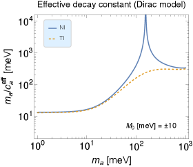
Fig. 13 shows the effective decay constant computed in the Dirac model. The Dirac model is given by expanding in Eq. (18) around . Using the same coefficients in the 3D TI model, we parametrize the Dirac model as
| (133) |
Finally, the dispersion relation of the AFM-type amplitude mode by using the parameters given in Ref. Li:2020fvr is given in Fig. 14. As in Fig. 5, the stability of this excitation is confirmed. In regions where and are large, the contours behave differently, but this is due to the relatively large value of , which is affected by the boundary in the wavenumber space integration. The behavior around is close to linear dispersion, which is simply because the gap is much smaller than eV.
References
- (1) J. Preskill, M. B. Wise, and F. Wilczek, Phys. Lett. B 120, 127 (1983).
- (2) L. F. Abbott and P. Sikivie, Phys. Lett. B 120, 133 (1983).
- (3) M. Dine and W. Fischler, Phys. Lett. B 120, 137 (1983).
- (4) D. J. E. Marsh, K.-C. Fong, E. W. Lentz, L. Smejkal, and M. N. Ali, Phys. Rev. Lett. 123, 121601 (2019), arXiv:1807.08810.
- (5) Y. Tokura, K. Yasuda, and A. Tsukazaki, Nature Reviews Physics 1, 126 (2019).
- (6) B. A. Bernevig, C. Felser, and H. Beidenkopf, Nature 603, 41 (2022).
- (7) J. Liu and T. Hesjedal, Advanced Materials 35, 2102427 (2023).
- (8) A. Sekine and K. Nomura, Journal of Applied Physics 129 (2021).
- (9) R. Li, J. Wang, X. Qi, and S.-C. Zhang, Nature Phys. 6, 284 (2010), arXiv:0908.1537.
- (10) K. Ishiwata, Phys. Rev. D 104, 016004 (2021), arXiv:2103.02848.
- (11) K. Ishiwata, Phys. Rev. B 106, 195157 (2022), arXiv:2206.00841.
- (12) L. Cao et al., Phys. Rev. B 104, 054421 (2021).
- (13) Y. Li et al., Phys. Rev. B 102, 121107 (2020), arXiv:2001.06133.
- (14) J. Wang, B. Lian, and S.-C. Zhang, Physical Review Letters 115 (2015).
- (15) M. N. Y. Lhachemi and I. Garate, Phys. Rev. B 109, 144304 (2024), arXiv:2311.10674.
- (16) B. Lake, D. A. Tennant, and S. E. Nagler, Phys. Rev. Lett. 85, 832 (2000).
- (17) A. Zheludev, K. Kakurai, T. Masuda, K. Uchinokura, and K. Nakajima, Phys. Rev. Lett. 89, 197205 (2002).
- (18) C. Rüegg et al., Phys. Rev. Lett. 93, 257201 (2004).
- (19) C. Rüegg et al., Phys. Rev. Lett. 100, 205701 (2008).
- (20) A. Jain et al., Nature Physics 13, 633–637 (2017).
- (21) T. Hong et al., Nature Physics 13, 638–642 (2017).
- (22) S. Hayashida et al., Phys. Rev. B 97, 140405 (2018).
- (23) S. Hayashida et al., Science Advances 5 (2019).
- (24) C. Herring and C. Kittel, Phys. Rev. 81, 869 (1951).
- (25) C. Herring, Phys. Rev. 85, 1003 (1952).
- (26) C. Herring, Phys. Rev. 87, 60 (1952).
- (27) J. König, T. Jungwirth, and A. H. MacDonald, Phys. Rev. B 64, 184423 (2001).
- (28) Y. Araki and K. Nomura, Phys. Rev. B 93, 094438 (2016).
- (29) H. Zhang et al., Nature Phys. 5, 438 (2009).
- (30) C.-X. Liu et al., Physical Review B 82 (2010).
- (31) G. Rosenberg and M. Franz, Physical Review B 85 (2012).
- (32) D. Kurebayashi and K. Nomura, Journal of the Physical Society of Japan 83, 063709 (2014).
- (33) J. Wang, B. Lian, and S.-C. Zhang, Phys. Rev. B 93, 045115 (2016), arXiv:1512.00534.
- (34) A. Sekine and K. Nomura, Phys. Rev. Lett. 116, 096401 (2016), arXiv:1508.04590.
- (35) J. Schütte-Engel et al., JCAP 08, 066 (2021), arXiv:2102.05366.
- (36) H. Ooguri and M. Oshikawa, Phys. Rev. Lett. 108, 161803 (2012), arXiv:1112.1414.
- (37) J. Zhang et al., Chinese Physics Letters 37, 077304 (2020).
- (38) S. Chigusa, T. Moroi, and K. Nakayama, JHEP 08, 074 (2021), arXiv:2102.06179.