Collaborative Ground-Space Communications via
Evolutionary Multi-objective Deep
Reinforcement Learning
Abstract
In this paper, we propose a distributed collaborative beamforming (DCB)-based uplink communication paradigm for enabling ground-space direct communications. Specifically, DCB treats the terminals that are unable to establish efficient direct connections with the low Earth orbit (LEO) satellites as distributed antennas, forming a virtual antenna array to enhance the terminal-to-satellite uplink achievable rates and durations. However, such systems need multiple trade-off policies that variously balance the terminal-satellite uplink achievable rate, energy consumption of terminals, and satellite switching frequency to satisfy the scenario requirement changes. Thus, we perform a multi-objective optimization analysis and formulate a long-term optimization problem. To address availability in different terminal cluster scales, we reformulate this problem into an action space-reduced and universal multi-objective Markov decision process. Then, we propose an evolutionary multi-objective deep reinforcement learning algorithm to obtain the desirable policies, in which the low-value actions are masked to speed up the training process. As such, the applicability of a one-time trained model can cover more changing terminal-satellite uplink scenarios. Simulation results show that the proposed algorithm outmatches various baselines, and draw some useful insights. Specifically, it is found that DCB enables terminals that cannot reach the uplink achievable threshold to achieve efficient direct uplink transmission, which thus reveals that DCB is an effective solution for enabling direct ground-space communications. Moreover, it reveals that the proposed algorithm achieves multiple policies favoring different objectives and achieving near-optimal uplink achievable rates with low switching frequency.
Index Terms:
Satellite networks, distributed collaborative beamforming, multi-objective optimization, virtual antenna arrays, deep reinforcement learning.I Introduction
While terrestrial networks, including the fifth-generation (5G) networks and Wi-Fi, have undergone extensive research and deployment, the current network architecture still faces challenges in providing coverage in remote areas and exhibits fragility during natural disasters [1]. In this case, non-terrestrial networks based on airborne movable elements, such as unmanned aerial vehicles (UAVs) and airships, have gained significant attention [2]. Recently, with the advancements in manufacturing processes, satellites become integral components of network architectures instead of only traditional roles in positioning and remote sensing, thereby significantly enhancing Internet coverage and disaster response capabilities [3, 4]. For instance, SpaceX develops the Starlink project to deliver global high-speed, low-latency broadband internet services [5]. Moreover, the third generation partnership project (3GPP) discussed the integration of satellite networks in Rel-18, including radio access networks, services, system aspects, core, and terminals [6].
Among various platforms, low Earth orbit (LEO) constellations, consisting of thousands of satellites, play a crucial role in satellite networks by offering advantages such as lower transmission delay compared to medium Earth orbit and geostationary Earth orbit satellites [7]. Leveraging LEOs has empowered various terrestrial devices to establish direct connections with satellite networks, which grants them extensive Internet access capabilities in remote areas [8]. However, some previously deployed terrestrial terminals may be energy-sensitive and equipped with coarse antennas. In such cases, the uplink transmission from these terminals to LEO satellites can be low-efficiency and only stable when the link distances are short. As such, the terminals have to switch satellites to connect frequently, resulting in the vexing problem of ping-pong handovers [9]. Thus, it is of significant importance to improve the terrestrial-satellite uplink quality for enabling ground-space direct communications.
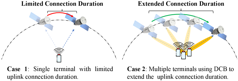
Distributed collaborative beamforming (DCB) can be introduced into terrestrial terminals to achieve this goal. Specifically, DCB treats separate systems such as these terminals as distributed antennas and simulates the beamforming process to produce a considerable transmission gain. This gain is beneficial to offset wireless fading even in long-range links between ground devices and satellites [10], thereby enhancing the corresponding transmission distance and the received signal strength. In this way, as shown in Fig. 1, we can adopt DCB to extend the connection duration of one satellite and enhance the uplink capabilities, thereby improving the uplink achievable rate and reducing the satellite switching frequency.
However, designing such a DCB-based terminal-to-satellite uplink communication system is a nontrivial task. First, the uplink transmission performance and energy efficiency of DCB are determined by transmit power allocation of terminals. As such, transmit powers of terminals should be carefully optimized according to the channel conditions [11]. Second, while DCB enhances transmission performance, the switching decision also needs to consider maximizing the uplink achievable rate and minimizing the satellite switching frequency. The relative importance of these two goals may vary across diverse scenarios, which means that the existing single-objective optimization and static methods in the literature (e.g., [12, 13]) are inappropriate. Finally, this system experiences periodicity from fixed satellite orbits, and suffers uncertainties and dynamics from wireless channel conditions. How to effectively discern the periodicity and deal with the dynamics in such systems are also imperative technical challenges. As such, addressing these challenges necessitates an innovative method absent from the current literature.
Accordingly, we aim to propose a novel DCB online multi-objective optimization approach that is more effective than existing work. The main contributions of this paper are summarized as follows:
-
•
DCB-based Terminal-to-satellite Uplink Communication Systems: We utilize DCB to enable and extend direct uplink communications between the terminals with coarse antenna and LEO satellites. This system can enhance the transmission gain of the terrestrial terminals, and thus enhance the uplink achievable rate and reduce the satellite switching frequencies of terrestrial terminals. To the best of our knowledge, such a joint optimization of satellite switching and DCB in satellite networks has not yet been investigated in the literature.
-
•
Long-term and Multi-objective Optimization Problem (MOP): We model the aforementioned system to explore its periodicity and dynamics. Our major finding is that the total terminal-satellite uplink achievable rate, total energy consumption of terminals, and satellite switching frequency are crucial objectives that conflict with each other. Accordingly, we perform a multi-objective optimization analysis and formulate an MOP to simultaneously optimize these concerned metrics. Then, we demonstrate that this MOP is non-convex and long-term, and requires a method with enhanced portability.
-
•
Innovative Multi-objective Deep Reinforcement Learning (DRL)-based Solution: Offline optimization methods are incapable of achieving the long-term optimum for this problem, while traditional reinforcement learning algorithms lack adaptability to different scenarios. To overcome this issue, we first reformulate the problem into an action space-reduced and universal multi-objective Markov decision process (MOMDP) to enhance its portability. Then, we introduce an evolutionary multi-objective DRL (EMODRL) algorithm and eliminate low-value actions to enhance its convergence performance. This algorithm is able to obtain multiple policies that represent different trade-offs among multiple objectives to accommodate diverse scenarios.
-
•
Simulation and Performance Evaluation: Simulation results demonstrate that the proposed EMODRL algorithm outmatches various baselines. Moreover, we find that DCB enables terminals that cannot reach the uplink achievable threshold to achieve efficient direct uplink transmission. In addition, it reveals that the proposed algorithm achieves multiple policies favoring different objectives and achieving near-optimal uplink achievable rates with low switching frequency.
The rest of this paper is organized as follows. Section II reviews the related research activities. Section III presents the models and preliminaries. Section IV formulates the optimization problem. Section V proposes the multi-objective DRL-based solution. Simulation results are presented in Section VI. Finally, the paper is concluded in Section VII.
II Related Works
In this work, we aim to propose a novel DCB-based terminal-to-satellite uplink communication method. This topic involves switching and handover in satellite networks and DCB optimization. Thus, we briefly introduce the related works of them as follows.
Switching and Handover in Satellite Networks In LEO satellites, the handover and switching schemes considering their mobility have been studied in previous literature. For instance, Wang et al. [8] proposed a handover optimization strategy based on a conditional handover mechanism to enhance service continuity in LEO-based non-terrestrial networks, in which an optimal target selection algorithm was designed to the maximum reward for each conditional handover mechanism. Moreover, Song et al. [14] proposed a channel perceiving-based handover management strategy to optimize the utilization of channels and dynamically adjust the data allocation strategy in space-ground integrated information networks. Nonetheless, the aforementioned studies concentrated on the timing and strategies of satellite switching and handover, and overlooked the opportunity to augment satellite connection duration by optimizing the transmission gain of terrestrial devices.
DCB Optimization: DCB has improved the transmission performance of various distributed systems, e.g., Internet-of-things (IoTs) [15], mobile wireless sensors [16], and automated guided vehicles [17]. Recently, UAVs and other aerial vehicles have incorporated DCB to enhance the efficacy of air-to-ground and air-to-air communications. Leveraging their three-dimensional (3D) mobility, UAVs can dynamically navigate to locations conducive to optimal DCB implementation and adjust communication parameters to fulfill diverse objectives. As such, prior research has explored the integration of DCB in UAV networks for purposes such as secure relay [18], confidential data transmission [19], data harvesting and dissemination systems [20], and others. Nevertheless, the aforementioned methods are not suitable for the considered scenario since they do not consider the periodic characteristics inherent in satellite networks, and also cannot address the trade-off between satellite switching and the transmission gain facilitated by DCB.
Thus, different from the existing works, we consider utilizing DCB to augment both the duration and transmission gain from terrestrial terminals to LEO satellites. Based on this, we seek to devise the switching and beamforming strategies of such systems to facilitate efficient terrestrial-to-satellite uplink transmission.
III System Models and Preliminaries
III-A Network Segments
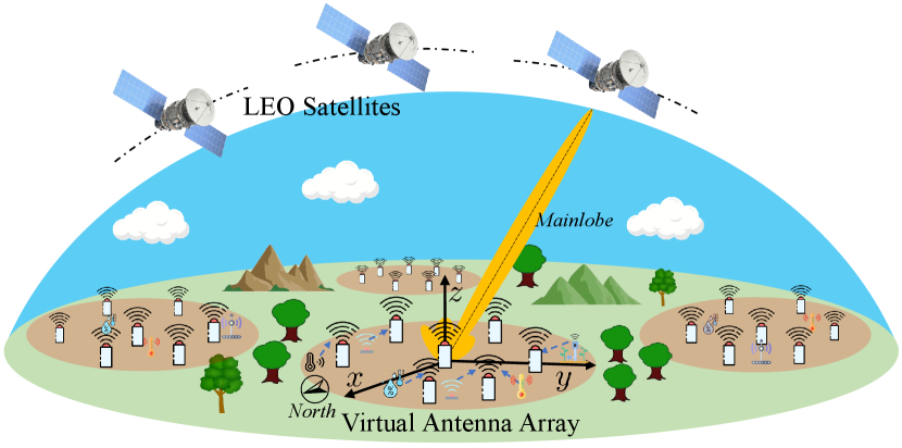
The terrestrial-satellite system under consideration is illustrated in Fig. 2, and it comprises the following elements:
-
•
A satellite network consisting of a constellation of LEO satellites . Each satellite may receive contents from terrestrial satellite terminals in its coverage and then transmit them to a data fusion center. These satellites are furnished with high-performance antennas with sufficient transmit power, and thus the downlink communications from satellites to terminals are efficient [21].
-
•
A terrestrial cluster comprising randomly distributed terminals. We consider that the geographical conditions (e.g., long intermediate distances, mountains, buildings, or other clustering methods [22]) naturally divide a large area into multiple ad hoc network clusters. Due to the link distance and channel conditions, intra-cluster communications are efficient, while the cooperation across clusters is unfeasible. These clusters may have varying numbers and distributions of terminals [23]. Thus, our primary focus is to investigate one of these clusters and propose a universal method which is applicable to such types of clusters. Without loss of generality, the cluster deploys a series of energy-sensitive and low transmission performance terminals, denoted as . Each terminal is able to collect data from IoT devices in coverage and needs to access the satellite network for data uploading. Due to constrained transmission resources, these terminals face challenges in establishing effective terrestrial-satellite uplinks, especially when the LEO satellite is remote.
Terrestrial-satellite links are affected by the elevation angle of the LEO satellite. Specifically, angles that are closer to result in shorter terminal-to-satellite distances, increasing the probability of a line-of-sight (LoS) connection. Conversely, angles below a certain angle (e.g., in S-band scenarios or in Ka-band scenarios) are unable to support data uploading [6].
We assume that each terminal can access a maximum of one LEO satellite at a time. Due to their insufficient transmit power, the terminals will form a virtual antenna array to obtain a higher gain. To maximize the uplink achievable rate and duration, we assume that the virtual antenna array introduces all the terminals within a cluster. Without loss of generality, we consider a discrete-time system evolving over timeline . At each time slot, only a subset of the LEO satellites have enough spectrum resources and suitable angles to receive data from the virtual antenna array. The available LEO satellite set at th time slot is denoted as . As such, the virtual antenna array needs to select one LEO satellite to connect and we denote the index of the connected LEO at the th time instant as . Note that we assume that the mainlobe of the virtual antenna array can track the motion of the connected satellite during the time slot.
We also consider a Cartesian coordinate system, where the locations of the th terminal and the connected LEO satellite at the th time slot are represented as and , respectively.
As such, the fixed communicable angles between terminals and satellites, coupled with the inherent orbital trajectories of satellites, introduce a certain periodicity to the system. Meanwhile, the limited spectral resources of satellites contribute to the uncertainty of availability, which brings dynamics to the considered system. In the following, we model the LEO satellite orbits and the communication process between the virtual antenna array and satellites to characterize the periodicity and dynamics within the system.
III-B LEO Satellite Orbit
LEO satellites are a category of satellites that orbit Earth at relatively low altitudes, typically ranging from approximately 160 to 2000 kilometers. These satellites complete one orbit around Earth in a relatively short period. Mathematically, the orbit of such LEO satellites can be determined by a tuple [24], which is detailed as follows:
-
•
Inclination Angle (): This angle represents the intersection between the orbital plane and the equator. In particular, an inclination angle exceeding indicates that the satellite’s motion is in the opposite direction to that of Earth’s rotation.
-
•
Right Ascension of Ascending Node (): This is the angle between the vernal equinox and the intersection of the orbital and equatorial planes.
-
•
Argument of the Perigee (): This angle is measured between the ascending node and the perigee, which is the point where the satellite is closest to Earth, along the orbital plane.
-
•
Eccentricity (): This parameter denotes the eccentricity of the orbital ellipse.
-
•
Semi-Major Axis (): This is a fundamental parameter used to describe the size and shape of an elliptical orbit. In the context of orbital mechanics, it is half of the length of the major axis, which is the longest diameter of the elliptical orbit.
-
•
True Anomaly (): This is the geocentric angle between the perigee direction and the satellite direction.
For the sake of simplicity and easy-to-access insights, we assume that the orbits of the LEO satellites are circular [25]. As such, the eccentricity () is set to 0 and the semi-major axis () is equal to the radius of the orbit . Likewise, due to the circular orbit, , in which is the altitude of satellite and denotes the radius of Earth. In this case, the angular velocity of this LEO satellite is given by , where is the gravitational constant, and is the mass of Earth. Following this, the orbital period can be calculated as .
By considering the discrete-time system, the timeline can be divided into multiple time slots with length . During different time slots, varies over time while other orbital parameters are fixed. Accordingly, let be the instantaneous orbital parameters of LEO satellite , the corresponding 3D Cartesian coordinate () in time slot can be given by
| (1) | ||||
As can be seen, the position of a LEO satellite is regularly changed with its orbital period according to its orbital parameters. As such, we can learn and exploit this feature when controlling key decision variables of the system.
III-C Virtual Antenna Array Model
In the virtual antenna array, all the terminals collaborate as one transmitter to send the same signals . By simulating traditional beamforming in array antennas, their emitted electromagnetic waves will be superposed at the LEO satellite, thereby achieving additional transmission gain. To this end, we consider that the terminals perform data sharing by using the existing methods in [26, 27], which have been demonstrated to have negligible costs. Moreover, aiming at making the signals precisely superposed at the LEO satellite, the terminals within the virtual antenna arrays are synchronized in terms of the time and initial phase via the synchronization methods in [28, 29].
As such, the sent signals are influenced by the characteristics of the channel between the terminals and LEO satellites. Specifically, we consider a remote rural scenario with no massive buildings that cause reflections and scattering. Moreover, due to the height of the satellite, the scattered signals cannot reach distant LEO satellites. In this case, we consider the channel model between the terminals and the satellites to be dominated by LoS. Thus, we introduce a channel model incorporating LoS path loss alongside random phases which may originate from the Doppler shift, device circuits, and other factors [30, 31]. Accordingly, the channel coefficient between the terminal and satellite at any given time slot can be expressed as:
| (2) |
where represents the channel power gain, is the propagation distance, is the path loss exponent, and denotes the channel phase shift at time slot . We assume that the terminals can detect the transmitted signals from the LEO satellites and obtain the quantized version of the actual channel state information via the method in [32], so that quantizing the estimated channel phase shift online with the traditional channel estimation methods [33].
Following this, as for any time slot , the transmitted signal of terminal is assumed as a circularly symmetric complex Gaussian (CSCG) random variable with zero mean and unit variance, which is given by , where and represent the transmit power and phase of terminal at time , respectively. To ensure that the signal can reach the satellite and superimpose with other signals, this transmit power should exceed a minimal threshold and below maximum power, and this constraint is given by , , .
Recall that the connected satellite at time slot is denoted as , the corresponding received signal is given by
| (3) |
where represents the additive white Gaussian noise at the connected satellite, modeled as a CSCG random variable with zero mean and variance . Recall that the terminals can perform online estimation of the channel phase shift, we assume that phase to maximize the received signal power at the satellite [31]. As such, if the angle between them supports transmission, the signal-to-noise ratio (SNR) of the satellite is given by [31]
| (4) |
Following this, the achievable rate from the virtual antenna array to the connected satellite can be expressed as follows:
| (5) |
where is the carrier bandwidth. As can be seen, the SNR and uplink achievable rate are primarily influenced by the instantaneous transmit powers of the terminals within the virtual antenna as well as the selection of the currently connected satellite at any time slot .
III-D Satellite Switching Model
For any time slot , the virtual antenna array needs to select one satellite to connect and upload the data. We assume that the virtual antenna array makes a decision at the beginning of each time slot whether to maintain the current satellite connection or select a new satellite connection. During this time slot, the virtual antenna array will always stay connected and automatically track the position of the satellite. We consider that the satellite divides its available bandwidth into distinct segments and allocates different bandwidths to individual receivers to mitigate interference. For the sake of simplicity, we assume that the satellite adopts the first-come first-served method, which means that once the allocated bandwidth is depleted, the satellite transfers to an unavailable state. This condition is clearly random to a virtual antenna array and thus modeled by a Bernoulli distribution with the probability [34, 35]. In this case, we let denote the index of the selected satellite at the timeline . This decision sequence variable could determine the uplink achievable rate and satellite switching frequency.
IV Problem Formulation and Analyses
In this section, we aim to formulate an optimization problem to improve the uplink transmission process of the virtual antenna array. We first highlight the main concern of the system, then present the decision variables and optimization objectives, and finally formulate a multi-objective optimization problem and give the corresponding analysis.
IV-A Problem Statement
In this work, we organize energy-sensitive terminals into a virtual antenna array to enhance terminal-to-satellite uplink transmission performance and minimize the satellite switching frequency to mitigate ping-pong handover issues. As such, the considered system involves three goals, i.e., improving the total uplink achievable rate obtained by LEO satellites, reducing the total corresponding energy consumption, and reducing the number of satellite switches.
At any time slot , the terminal transmit powers used to communicate with the selected satellite determines the uplink achievable rate. As such, the satellite selection and the transmit powers of terminals are interdependent and coupled. Simultaneously, the transmit powers of the terminals also impact their energy consumption, while the sequential decision-making order of the satellite selection affects the satellite switching frequency. Thus, these optimization objectives have conflicting correlations. Accordingly, the coupling of variables and mutual influence of objectives require a multi-objective optimization formulation. The decision variables are introduced as follows.
We define these decision variables and seek to jointly determine them: (i) , a matrix consisting of continuous variables denotes the transmit powers of terminals over time slots for performing DCB. (ii) , a vector consisting of discrete variables represents the index of the selected satellite during the timeline. In what follows, we give the expression of the considered optimization objectives.
Optimization Objective 1: The primary objective is to improve the uplink achievable rate from the virtual antenna array to LEO satellites over the total timeline. As such, the first optimization objective is given by
| (6) |
Optimization Objective 2: When engaging in terminal-to-satellite communications, the transmit powers of the terminals directly determine their energy consumption. Given that the terminals are energy-sensitive and have limited supply energy, our second optimization objective is to minimize the total energy consumption of the terminals, which is designed as
| (7) |
Optimization Objective 3: To maximize the uplink achievable rate and minimize the corresponding energy consumption, the virtual antenna array needs to select an appropriate satellite from the satellite list as the receiver. However, frequent satellite switching will lead to ping-pong handover issues and incur additional link costs. Hence, the third objective is to minimize the number of satellite switches (i.e., frequency). Let be the number of satellite switches at time slot , and evolves as follows:
| (8) |
Following this, our third optimization objective is designed as
| (9) |
According to the three optimization objectives above, our optimization problem can be formulated as follows:
| (10a) | ||||
| s.t. | (10b) | |||
| (10c) | ||||
| (10d) | ||||
IV-B Problem Analyses
The problem () has the following properties. First, the problem () is non-concave. This is due to the fact that its first objective function involves coupled variables comprising both continuous decision variables () and integer decision variables (). Second, the problem () contains long-term optimization objectives influenced by the periodicity of satellite orbits and the dynamic satellite availability status. Finally, the problem () is an MOP with conflicting optimization objectives. For instance, under given channel conditions, improving the uplink achievable rate necessitates increasing the transmit powers of the terminals (i.e., ), resulting in the more energy consumption. Likewise, if the transmit powers of the terminals are fixed, consistently selecting the satellite with the best channel condition and distance will increase the satellite switching frequency.
Hence, the problem () is a non-convex mixed-integer programming problem with a long-term optimization goal, incorporating dynamics and periodicity. This complexity renders it unsuitable for offline optimization methods such as convex optimization and evolutionary computing. Additionally, the problem () is characterized as an MOP with conflicting objectives. The importance of these objectives varies in different applied scenarios and occasions. For instance, when the terminals are at low energy levels, the decision-maker seeks an energy-efficient deployment policy. Likewise, if the current data needed to be uploaded is large, the decision-maker prioritizes a policy that can maximize the uplink achievable rate. Thus, it is desirable to have a method that can achieve multiple policies for the decision-maker to select. Furthermore, the status information of such systems (e.g., channel conditions) may not always known accurately. Thus, it is necessary to have an online and real-time response method for solving the problem. Finally, while we have formulated a problem for one cluster with a fixed number of terminals, we also aim for the method could be easily adaptable to the clusters with varying terminal numbers with minimal modifications. Therefore, we require a method with enhanced portability.
In this case, DRL can be a promising online algorithm capable of learning periodicities and adapting to the dynamic [36]. The aforementioned reasons motivate us to propose a DRL approach capable of addressing MOPs for solving the formulated problem.
V Multi-objective DRL-based Method
In this section, we propose a multi-objective DRL-based method for solving the formulated problem. We begin by presenting the inherent challenges of applying traditional DRL to solve the problem.
-
•
Lack of Portability: In DRL, the set of available output actions is fixed, and once they significantly change, the DRL model needs to be re-trained. Thus, when utilizing DRL to solve our problem, a change in the number of terminals will mandate model retraining, which decreases its practicality and portability in real-world systems.
-
•
Absence of Alternative Trade-off Policies: hen dealing with multiple optimization objectives, DRL methods often combine multiple optimization objectives into one reward function according to their importance and roles. Then, DRL methods will derive one policy that is the most suitable for this reward function. In this case, decision-makers lack alternative trade-off policies to cater to various scenarios that prefer different optimization objectives. The obvious changes in the importance of optimization objectives require a redesign of the reward function and retraining of the DRL model, thereby diminishing its practicality.
-
•
Challenges in Fast Learning and Convergence: Due to the large number of satellites and their rapidly changing availability status, the traditional DRL algorithm may not swiftly acquire strategies and converge effectively.
Accordingly, our main focus is to ensure the availability of the trained DRL model under slight changes in the terminal number, and achieve multiple policies that can cover optimization objective importance varying. To this end, we will first transform our problem into an action space-reduced and more universal MOMDP.
V-A MOMDP Simplification and Formulation
An MOMDP extends the Markov decision process (MDP) framework, which can be represented by a tuple . In the tuple, , , , , and denote state space, action space, state transition probability, discount factor, and initial state distribution, respectively. Different from MDP, in MOMDP is a reward vector, in which is the reward for the th objectives. As such, some DRL methods modified for multi-objective optimization can combine the reward vector into one reward function in different forms and thereby obtain the corresponding policies that represent different trade-offs.
In general, the decision variables of an optimization problem (such as and ) will be the actions when this problem is represented as an MOMDP. Thus, the action space of the MOMDP should contain the transmit power of each terminal (i.e., ). As aforementioned, this approach will decrease the portability of the method since the model needs to be re-trained when the number of terminals changes. Moreover, a large number of terminals may lead to an explosion in the possible combinations within the action space. In this case, we aim to transform the actions related to , so that mitigating the impact of terminal number changes within the virtual antenna array and reducing the action space. The main challenge of this task is to ensure the transformed actions are efficient and can still determine the trade-offs between the uplink achievable rate and energy consumption.
V-A1 Action Transition
To ensure the availability of the DRL model when terminal numbers vary, the key point is to fix the action dimension associated with the transmit powers of the terminals. To this end, we first derive the relationship between the importance of the objectives 1 and 2 with the optimal transmit powers of the terminals. Specifically, we only consider one-time slot optimization and let and be the weights of these two objectives. Then, we can give a new optimization problem as follows:
| (11) | ||||
| s.t. |
where the first term is to minimize the energy consumption of the virtual antenna array (i.e., ) while the second term is to maximize the SNR (SNR and achievable rate increase in tandem, and as such, the second term can be representative of ), and is a normalization parameter that puts the two terms in the same order of magnitude. As such, if we solve the problem optimally, the instantaneous transmit powers of terminals that are the most suitable for the objective weights and can be obtained.
Lemma 1.
In the considered scenarios and feasible set of (), the problem is convex.
Proof.
Following this, the Hessian matrix of , denoted by , is given by
| (14) |
As can be seen, the values on the diagonal of the matrix are always greater than zero. In our considered scenario, all terminals are deployed within a concentrated area. The maximum distance between terminals is significantly smaller than the satellite-terminal distance. Thus, the distances from the satellite to each terminal, i.e., (), can be treated as equal. Moreover, the scenario involves the use of low-performance antenna terminals for satellite connection. For the signal to successfully propagate to the satellite, these low transmission performance terminals need to employ almost maximum transmit power. In such cases, , implying that the disparity among the transmit powers () is relatively small and can be neglected compared to other parameters shown in Eqs. (12) and (13). Thus, the values on the diagonal are much larger than the values on the off-diagonal. In this case, the Hessian matrix is positive semidefinite, and the problem is convex.
Accordingly, can be solved optimally or near-optimally by solvers. Consequently, the instantaneous transmit powers of terminals can be well-determined according to the objective weights and . In this case, we can use the fixed-dimension weights and instead of the transmit powers of terminals as the actions of the MOMDP, which reduces the impact of terminal number varying.
Following this, the computing resources of the considered DCB-based terminal-to-satellite uplink communication are often constrained, which needs a swift training process for flexible parameter tuning and rapid model deployment. To accelerate the training process, we discrete the weights associated with optimization objectives 1 and 2 by using equidistant discretization [37]. As such, the DRL algorithms only need to consider a finite number of action options thereby facilitating the training speed.
In particular, let denote the alternative weight set, and then and can be established as follows [37]:
| (15) |
Hence, the action concerning the transmit powers of terminals can be transformed to choose various alternative weight schemes within . This transformed action has a fixed dimension even if the terminal number changes and can represent the optimal or near-optimal transmit powers of terminals.
V-A2 MOMDP Formulation
Benefiting from the simplification above, we can re-formulate the optimization problem shown in Eq. (10) as an action space-reduced and more universal MOMDP. The key elements of the MOMDP are given as follows:
-
•
State Space: We assume the terminals possess a precise timer and maintain satellite orbit data, thus acquiring accurate real-time satellite positions. Simultaneously, the log system of the virtual antenna array can store the index of the last-connected satellite. Note that we employ accurate real-time satellite positions to derive the transmit powers of terminals without inputting them into the DRL model. Consequently, the observable state at time slot of the virtual antenna array is given by
(16) -
•
Action Space: As aforementioned, the virtual antenna array can select the trade-off schemes in instead of using the DRL model to determine the transmit powers of terminals at different time slots. Except for that, the virtual antenna array should select one satellite to connect at any time slot. Thus, the actions that can be adopted at time slot by the virtual antenna array contain
(17) where indicates the selected scheme from at time slot .
-
•
Reward Function: In DRL models, the environment furnishes immediate rewards after an action is performed, and then the agent adjusts its actions and learns the optimal policy according to the reward. Thus, it is essential to design a reasonable reward for enhancing the solving performance of such DRL models. To achieve long-term multi-objective optimization, the reward vector is
(18) where , , and are three normalization parameters intended to bring them into the same order of magnitude. Additionally, if , then ; otherwise, . Moreover, is a parameter indicating whether the satellite changes (i.e., denotes changes and vice versa). As can be seen, these three terms denote different objectives shown in Eq. (10).
Based on this, we obtain an MOMDP in which the reward is a vector containing multiple objective rewards. Next, we aim to propose a novel multi-objective DRL method to obtain several long-term policies representing different trade-offs.
V-B EMODRL-based Solution
The proposed EMODRL-based solution consists of multiple learning tasks, in which each task represents a specific trade-off among different optimization objectives. Following this, these tasks are collaboratively performed and learned by multiple agents. Through cooperation, the agents jointly converge towards Pareto optimal policies, thereby handling the formulated MOMDP. In what follows, we initially present the behavior and logic of an individual task and agent, and then delve into the cooperation of multiple learning tasks.
V-B1 Learning Task and Enhanced Dueling DQN Agent
In the proposed EMODRL-based solution, the th learning task can be represented as a tuple , where (, ) is a weight vector for optimization objectives and is the policy that seeks to achieve the best cumulative reward () under the current objective weights.
We employ the dueling deep Q network (D3QN) [38] to learn the qualified policy (). Specifically, D3QN is an extended version of DQN, and both of which are value-based reinforcement learning and utilize a neural network to store state and action information, i.e., Q-value (). Their primary objective is to discover the optimal policy and acquire the corresponding optimal state-action values , expressed as . Different from DQN, D3QN defines the Q-value as the sum of the state value and the advantage values, i.e.,
| (19) |
where represents the value of being in state , and represents the advantage of taking action in state [38]. By separately estimating the state value and advantage values, the D3QN agent model can discern and prioritize actions more effectively, leading to improved learning and decision-making. Based on this, D3QN employs epsilon-greedy exploration during action selection. This strategy balances exploration and exploitation by selecting the action with the maximum Q-value with probability and choosing a random action with probability .
However, the action space of the MOMDP encompasses some deterministic low-reward actions, and the epsilon-greedy cannot avoid such actions and may make meanless attempts. This inadequacy may hinder the D3QN agent from swiftly acquiring strategies and converging effectively. To overcome this issue, we seek to enhance the action selection strategy of D3QN. Specifically, the optimal policy is characterized by the exclusion of the unavailable satellites imposed by constraints on angle and spectrum resources from the action set . This is due to the fact that switching to an unavailable satellite will not get positive rewards in both the current step and future moments. Based on this, we propose a legitimate action select method to mask such low-reward actions. Specifically, we define the legitimate action set at the th time slot as , in which the actions of switching unavailable satellites have been excluded. Then, we propose an epsilon-greedy scheme as follows:
| (20) |
Following this, we can use this exploration scheme to sample data and train for minimizing the loss function, thereby achieving the qualified network parameters . The loss function is as follows:
| (21) |
where and , in which and are the target value and target advantage, respectively [38].
Next, we will present the learning tasks and introduce the interaction of these enhanced D3QN agents.
V-B2 EMODRL-ED3QN Framework
In this part, we present an EMODRL-enhanced D3QN (EMODRL-ED3QN) to obtain a set of Pareto near-optimal policies by learning from the feedback of the environment.
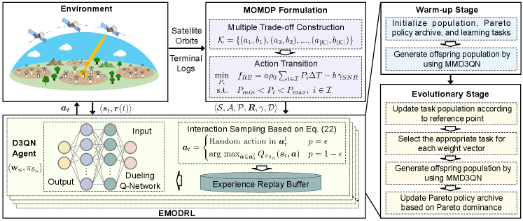
As shown in Fig. 3, EMODRL-ED3QN has the same structure as the multi-objective DRL frameworks in [39, 40], which has warm-up and evolutionary two stages. In the warm-up stage, EMODRL-ED3QN generates learning tasks and generates the initial task population by using the multi-task ED3QN scheme shown in Algorithm 1. The evolutionary stage will update the task population, and the Pareto policy archive based on the continuously generated offspring population. These two stages are detailed as follows.
Warm-up Stage: This stage stochastically generates a set of learning tasks which are defined as . Note that these tasks share the same state space, action space, and reward vector, but have different objective weight vectors and neural network parameters. First, the weight vectors of these tasks are assigned as , in which they are evenly distributed and sampled from a unit simplex [14]. Then, we randomly initialize Q-value networks . As such, can make decisions according to the Q-value networks and the weighted reward .
Next, we utilize the multi-task ED3QN scheme to generate the initial task population. As illustrated in Algorithm 2, this multi-task ED3QN approach allows all learning tasks to gather data from the environment and adjust network parameters according to the main steps of the ED3QN agent. The learning tasks with the adjusted network parameters are the generated offspring task population.
As such, we can obtain a set of learning tasks with well-initialized policies, and the process of the evolutionary stage can unfold as follows.
Evolutionary Stage: This stage explores better strategies by iteratively updating the task population. Each iteration contains three steps that are task population updating, Pareto policy updating, and offspring population generating.
As for task population updating, we need to update the task population according to the newly generated offspring population (As shown in Algorithm 3). In this case, it is essential to distinguish the nondominated policies and keep the population diversity. Thus, we introduce the buffer strategy [14] to reasonably update . Specifically, multiple buffers are set to store , in which and are defined as their total number and capacities, respectively. As such, the objective performance space is segmented into buffers, each capable of storing up to policies. We can set a reference point [40] to prioritize these policies within the same buffer.
Accordingly, for any given buffer, tasks are sorted in descending order based on their distances to . If the number of tasks exceeds , only the first tasks in that buffer are retained. Following this, the learning tasks from all buffers collectively constitute a new task population.
As for Pareto policy updating, a Pareto archive is utilized to retain nondominated policies discovered during the evolutionary stage. Specifically, this Pareto archive undergoes an update according to the offspring population . For the ED3QN policy of each task in , the policies dominated by are excluded, and is added to the Pareto archive only if no policies in the Pareto archive dominate (see step 11 of Algorithm 1).
As for offspring population generating, we choose the optimal task from and still use the multi-task ED3QN approach to obtain the offspring task population. Specifically, we evaluate the objective function values of each policy within . Then, for a given weight vector , we determine the best learning task in based on and () (as shown in Algorithm 4). Finally, the selected learning tasks are incorporated into . We derive by executing multi-task ED3QN (see Algorithm 2) with and as its input, where represents the predefined number of task iterations.
This stage terminates if the predefined number of evolution generations are completed. In this case, all non-dominated policies stored in the Pareto archive will be output as the Pareto near-optimal policies for the formulated MOMDP as well as the optimization problem. These policies represent different trade-offs between the total uplink achievable rate, total energy consumption of terminals, and total satellite switching number. As such, the decision-makers can select one policy from them according to the current requirements and concerns.
V-B3 Complexity Analysis
We first consider the time complexity of the training EMODRL-ED3QN model. Specifically, in both the warm-up and evolutionary stages, the major complexity comes from the step of generating offspring population which involves the training of neural networks. Compared with this step, other steps (e.g., steps 8, 9, and 11 in Algorithm 1) are considered trivial and can be disregarded.
As shown in Algorithm 2, MMD3QN generates the offspring population, and its time complexity mainly depends on the training of neural networks. MMD3QN iteratively optimizes each learning task in the task set for times (i.e., steps 2-8 in Algorithm 2), where denotes the number of task iterations. Let denote the number of collected data, and be the number of epochs for training the Q-value network. Note that the implemented Q-value network is the fully connected neural network, which consists of an input, an output, and fully connected layers. The numbers of neurons in the input and output layers are 2 and 2, respectively. Let denote the number of neurons in the th fully connected layer, with and . Consequently, the time complexity of MMD3QN is expressed as [39].
By considering the predefined number of maximum evolution generations (), the time complexity of training EMODRL-ED3QN is .
Moreover, we analyze the time complexity of using the trained EMODRL-ED3QN. Since EMODRL-ED3QN achieves multiple alternative policies to match the current preference, using EMODRL-ED3QN does not need transfer learning or other tuning. As such, the selected policy can quickly generate a solution to the problem through simple algebraic calculations. In this case, the time complexity of using the trained EMODRL-ED3QN is , where is the number of time slots [39].
VI Simulations and Analyses
In this section, we conduct key simulations to evaluate the performance of the proposed EMODRL-ED3QN-based method for solving the formulated optimization problem.
VI-A Simulation Setups
VI-A1 Scenario Settings
In this work, we consider a terrestrial terminal to LEO satellite communication scenario, which includes the LEO satellite, terrestrial terminal, and communication-related parameters. First, we set up 110 periodically operated LEO satellites, of which 80 LEO satellites at an altitude of m and 30 LEO satellites at an altitude of m. Note that most of them are around the equatorial orbit and some of them have an inclination angle around , and the satellites in the same orbit are evenly distributed in this orbit [41, 25]. Second, we consider a terrestrial terminal area located near the equator, in which exists 10 terrestrial terminals and several sensors. Note that these devices can perform efficient information sharing and communication within the area. Finally, the carrier frequency, minimum to maximum transmit powers of each terminal, path loss exponent, and total noisy power spectral density are set as 2.4 GHz, 1-2 W, 2, and -157 dBm/Hz, respectively.
Additionally, we consider a timeline of 60 minutes. The radius of Earth , gravitational constant , and mass of Earth are set as m, , and kg, respectively.
VI-A2 Algorithm Settings
In the proposed EMODRL-ED3QN, we set the number of the learning tasks as 10. In addition, the maximum evolution generations , the iteration number during the warm-up stage , and the iteration number for training each task are set as 300, 80, and 20, respectively. Finally, the number of performance buffers is designed to 50, and each buffer size is set to 2. For each learning task, the Q-value network has two fully connected layers with 2048 neurons and the tanh function serves as the activation function. Moreover, the learning rate is and the discount factor is . The replay buffer size and batch size are set as and , respectively.
VI-A3 Baselines
To demonstrate the performance of the proposed EMODRL-ED3QN, we introduce and design various comparison algorithms and strategies as follows:
-
•
Non-DCB strategy: This strategy does not introduce DCB technology and only adopts one single terrestrial terminal to connect to the satellite directly.
-
•
Achievable rate greedy policy (ARGP): ARGP refers to the policy that any terminal employs the maximum transmit power and selects the satellite with the utmost uplink achievable rate at any time slot . Note that ARGP achieves the upper bound of optimization objective 1.
-
•
State-of-the-art baseline algorithms: We design EMODRL-D3QN, EMODRL-Noisy-DQN, EMODRL-DDQN, EMODRL-PPO, EMODRL-TD3, and EMODRL-SAC as the baseline algorithms. Note that they are the variants of D3QN, Noisy-DQN [38], double DQN (DDQN) [42], proximal policy optimization (PPO) [43], twin delayed deep deterministic policy gradient algorithm (TD3) [44], and soft actor-critic (SAC) [45], respectively. We develop them by introducing the proposed evolutionary multi-objective reinforcement learning and multi-task frameworks for dealing with the formulated MOMDP.
As such, the comparison with non-DCB strategy shows the effectiveness of introducing DCB, the comparison with ARGP can assess the effect of the proposed evolutionary multi-objective DRL framework, and the comparison with other EMODRL algorithms can illustrate the optimization efficiency of EMODRL-ED3QN. In the following comparisons, we consider the average optimization objective values of these algorithms over timelines (i.e., , , and ) as a performance metrics.
VI-B Performance Evaluation
VI-B1 Comparisons with Non-DCB Strategy
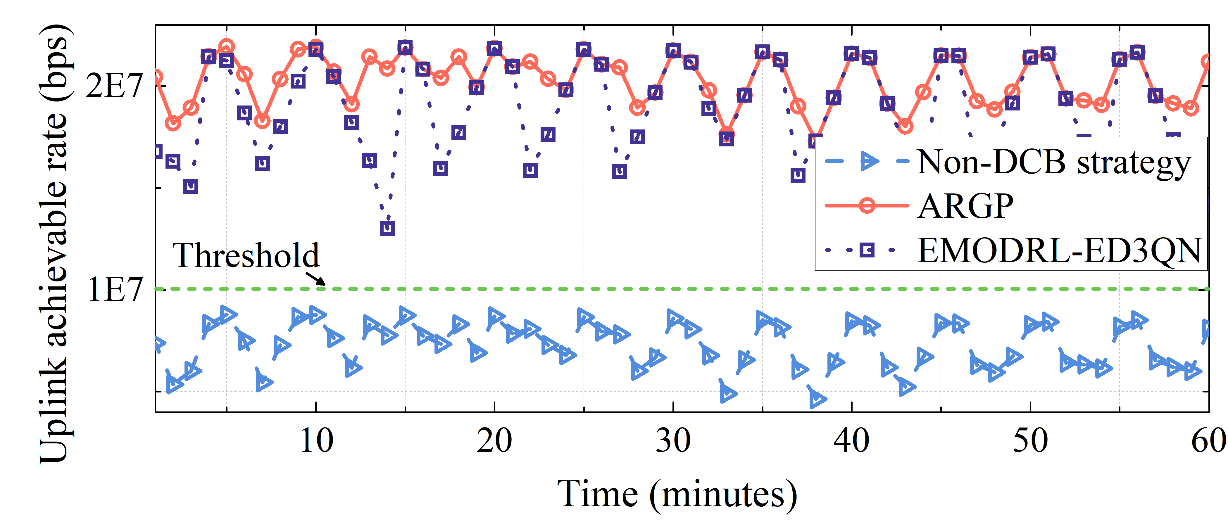
In this part, we compare the DCB-based policies and the non-DCB strategy to illustrate the effectiveness of the considered DCB-based uplink communication approach. Specifically, uplink achievable rates obtained by a policy of EMODRL-ED3QN, ARGP, and non-DCB strategy at each time slot are shown in Fig. 4. As can be seen, ARGP and EMODRL-ED3QN consistently surpass the threshold for uplink communication. In contrast, the non-DCB strategy struggles to attain an uplink achievable rate above the threshold. Moreover, the EMODRL-ED3QN policy achieves performance closely aligned with the upper bound (i.e., ARGP) at every time slot. These results show that the DCB-based uplink communication approach and EMODRL-ED3QN policy are both reasonable and suitable for the considered scenario.
VI-B2 Comparisons with Different Baselines
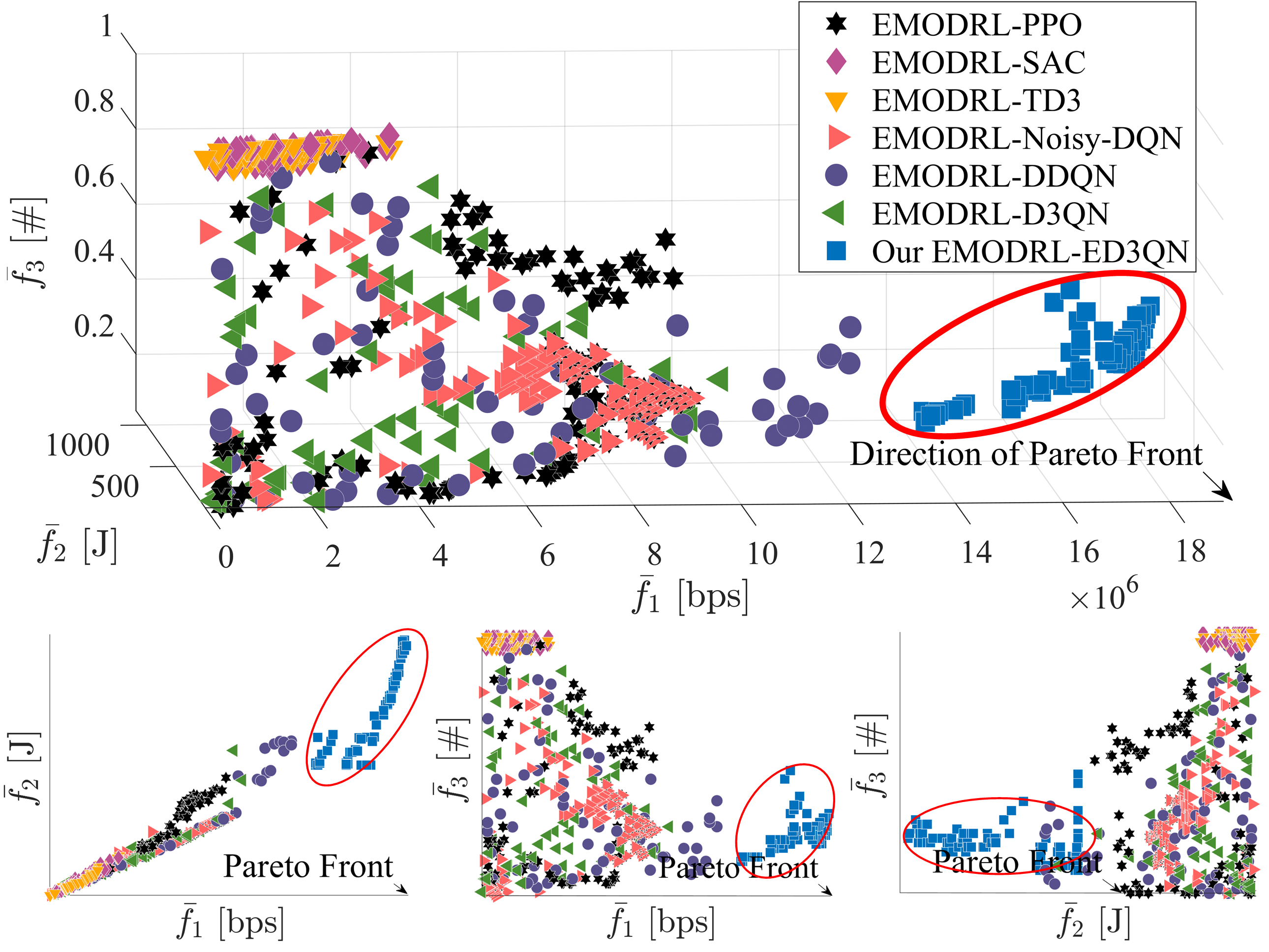
We first evaluate the trade-offs obtained by the proposed EMODRL-ED3QN in solving the formulated problem. As shown in Fig. 5, we show the trade-offs among the considered three objectives obtained by multiple EMODRL baselines. As can be seen, all these algorithms obtain a set of Pareto policies with wide coverage among the considered three objectives. Thus, the considered EMODRL framework is effective and can obtain multiple policies that weigh each other. Moreover, EMODRL-ED3QN, EMODRL-Noisy-DQN, and EMODRL-DDQN outperform other comparison algorithms. This is because the three algorithms are offline reinforcement learning methods, which may save more periodic information in their replay buffer, thereby facilitating the learning of the periodicity of the considered system. Additionally, we can see that the proposed EMODRL-ED3QN outmatches other baselines. The reason is that the proposed legitimate action select method can well-balance the exploration and exploitation of the algorithms. Moreover, the structure of the selected D3QN is also the most suitable for the designed MOMDP and legitimate action select method, and thus enables the algorithm to approach optimal performance closely.
Second, we select one policy from the Pareto policy set of each algorithm for further comparisons and analyses. In most cases, the uplink achievable rate from the terrestrial terminals to LEO satellites is the most concerned optimization objective. As such, we choose the policy with the best optimization objective 1 from the Pareto policy set as the final policy. In this case, the numerical results in terms of the considered optimization objectives are shown in Table I. As can be seen, the proposed EMODRL-ED3QN achieves a similar objective 1 and much lower objectives 2 and 3 with the ARGP policy. This demonstrates that the proposed EMODRL-ED3QN uses lower energy consumption and satellite switching numbers to obtain a nearly optimal uplink rate. Moreover, compared with other comparison policies, EMODRL-ED3QN has a better balance among the three optimization objectives. Note that although EMODRL-PPO, EMODRL-TD3, and EMODRL-SAC achieve better optimization objectives 2 and 3, their optimization objective 1 is inadequate, making them unsuitable for terrestrial-to-satellite communication scenarios. Therefore, we can illustrate that EMODRL-ED3QN is most suitable for the considered scenario and can mitigate the ping-pong handover issue.
| Method | [bps] | [J] | [] |
|---|---|---|---|
| ARGP | |||
| EMODRL-PPO | |||
| EMODRL-SAC | |||
| EMODRL-TD3 | |||
| EMODRL-Noisy-DQN | |||
| EMODRL-DDQN | |||
| EMODRL-D3QN | |||
| Our EMODRL-ED3QN |
VI-B3 Policy Evaluations
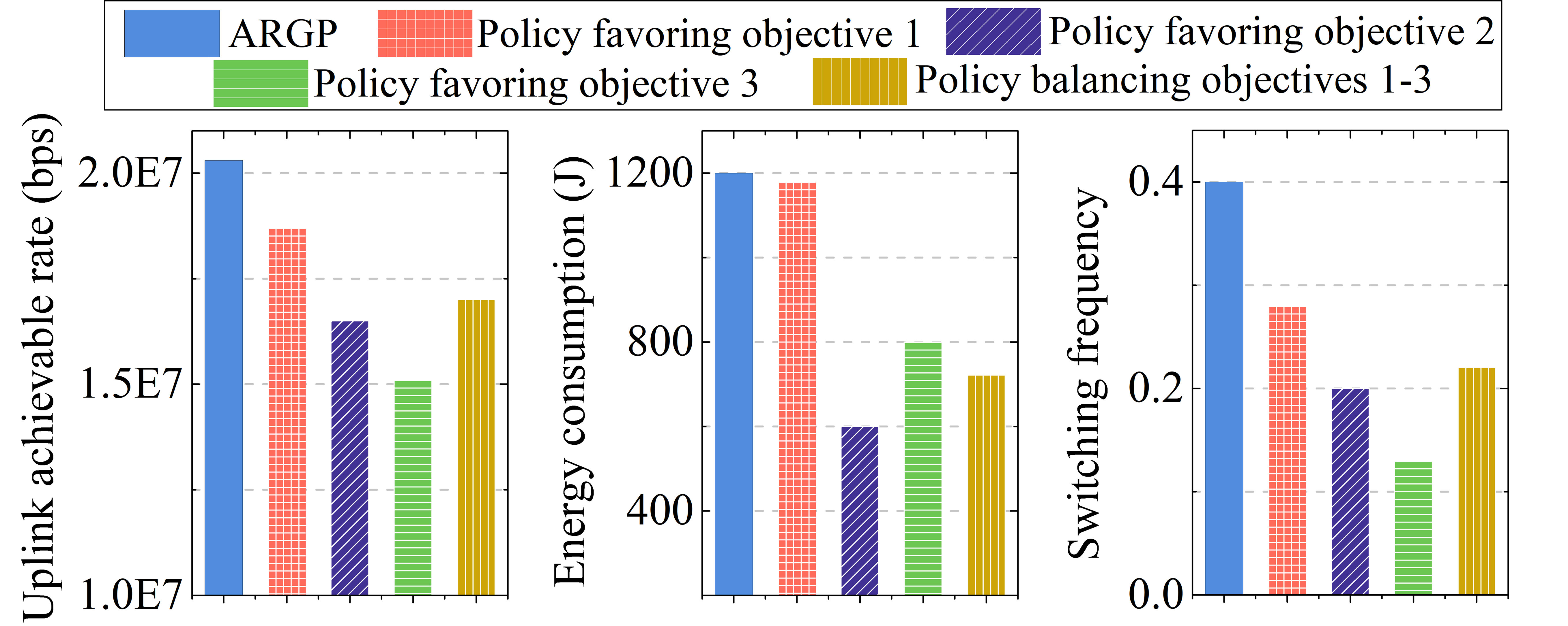
We first select different trade-off policies from the Pareto policy archive of EMODRL-ED3QN to illustrate the diversity performance of the obtained policy set. Specifically, we select four different trade-off policies which are policy favoring objective 1, policy favoring objective 2, policy favoring objective 3, and policy balancing objectives 1, 2, and 3, and the optimization objective values of these policies are shown in Fig. 7. It can be seen that the four policies all have obvious differences and show different objective tendencies when solving the formulated problem. In addition, these policies all achieve slightly weaker objective 1 but much better objectives 2 and 3 than ARGP. These results show that the policy set obtained by EMODRL-ED3QN has strong diversity.
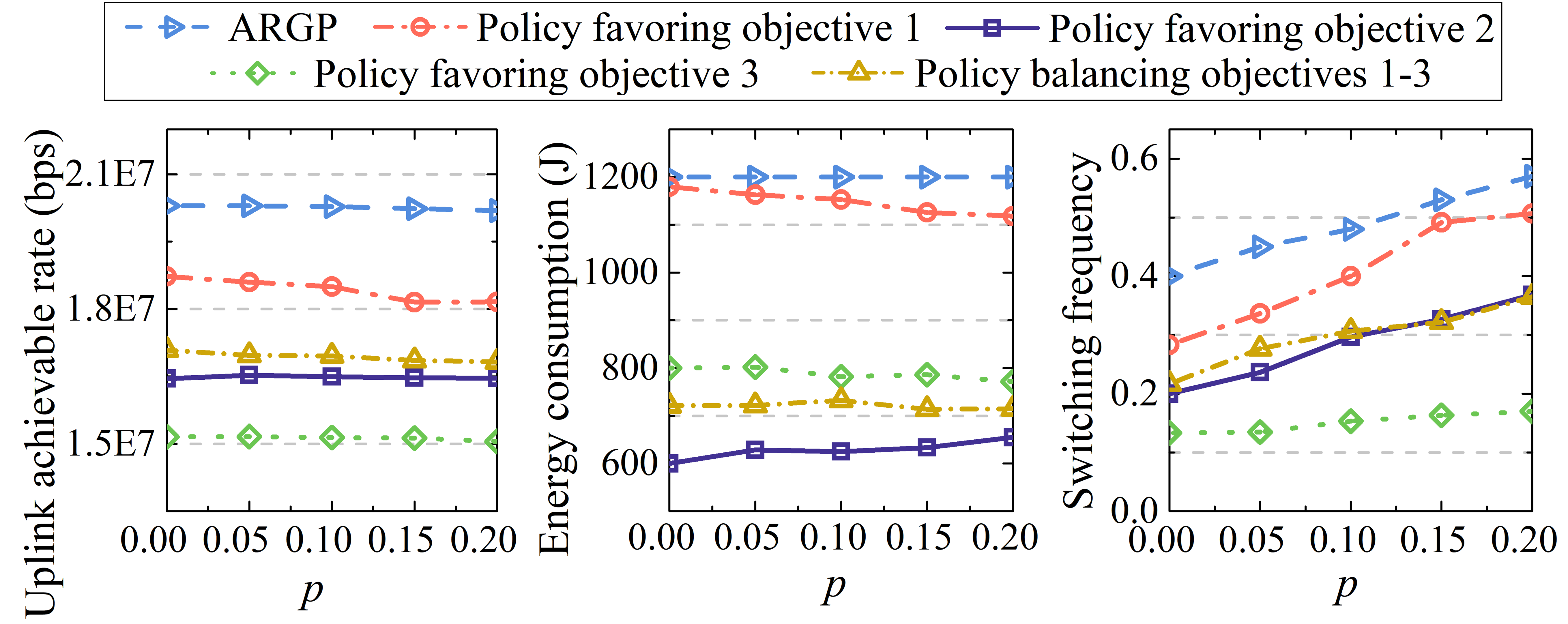
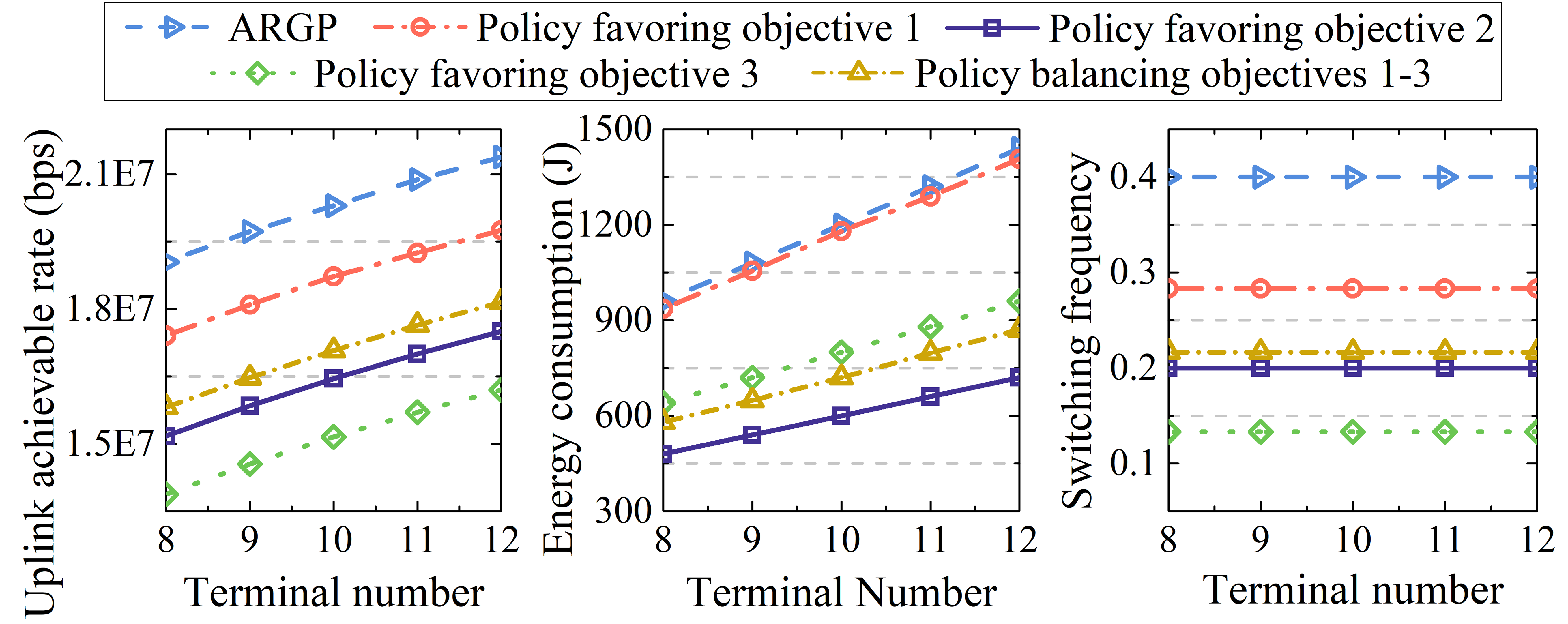
Then, we evaluate the impacts of scenario changes on the policies obtained by the proposed EMODRL-ED3QN. Specifically, the satellite unavailable probability may have a significant effect on these policies. Thus, we depict the changes in the three optimization objectives with satellite unavailability probability in Fig. 6(a). We can observe that the policies still show different objective tendencies and no significant deterioration occurred compared with ARGP. Moreover, as aforementioned, we seek to propose a method in which one-time training can accommodate various terminal numbers. Fig. 6(b) shows the performance of these trained policies changed with the terminal numbers. As can be seen, the policies still show obvious objective tendencies and achieve good performance. The reason is that the proposed legitimate action select method can enable EMODRL-ED3QN to fully explore and utilize the high-value action space and obtain more valuable trade-off policies. Thus, one-time training of the EMODRL-ED3QN can obtain multiple trade-off policies with portability.
VI-B4 Ablation Simulations
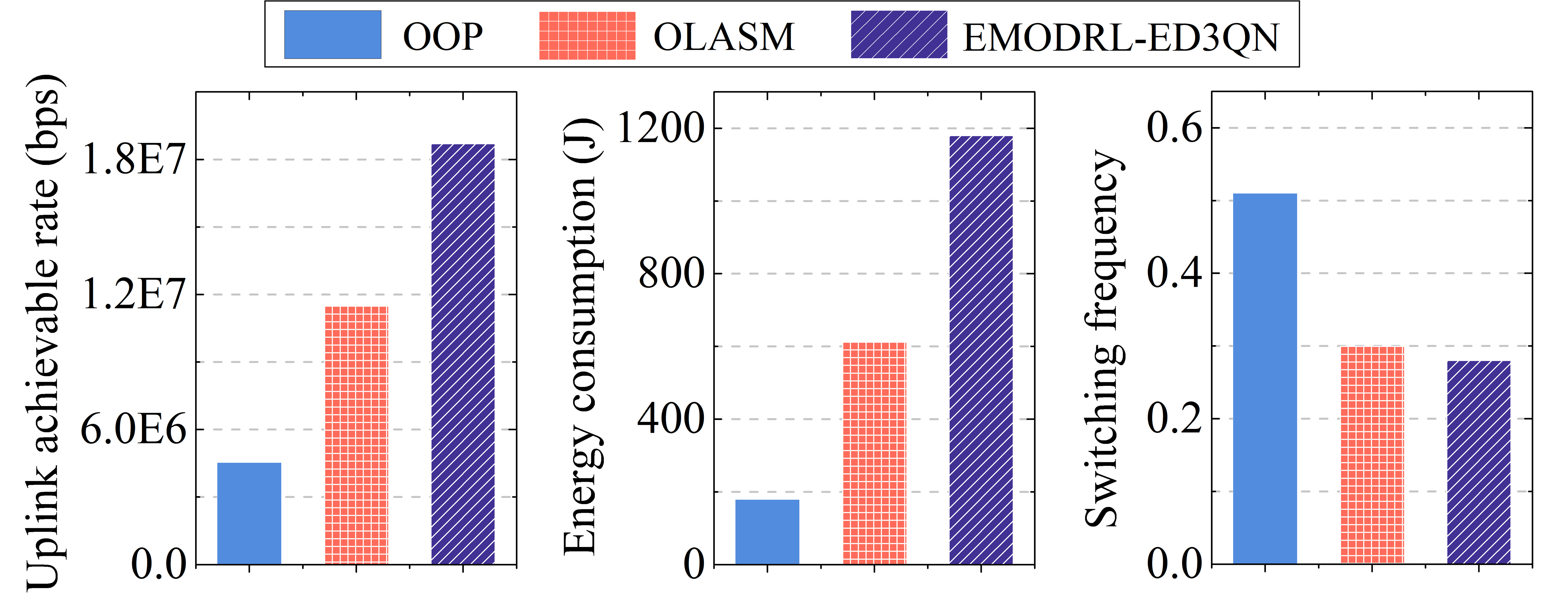
Ablation simulations are conducted to illustrate the effectiveness of the proposed enhanced methods. Specifically, we consider two strategies that are optimization without optimized (OOP) and optimization without legitimate action select method (OLASM). In OOP, the transmit power of each terrestrial terminal is not optimized and randomly generated. In OLASM, the proposed legitimate action select method is not considered. Accordingly, the comparison results are shown in Fig. 8. As can be seen, the proposed EMODRL-ED3QN is significantly better than other ablated strategies. This shows that the proposed enhanced methods are effective and can boost the training performance of the traditional DRL algorithm in such scenarios.
VII Conclusion
This paper investigated a DCB-based joint switching and beamforming terminal-to-satellite uplink communication system. Specifically, we used the low transmission performance terminals as a virtual antenna array to enhance terminal-to-satellite uplink achievable rates and duration. In this system, we formulated a long-term optimization problem to improve the total uplink achievable rate, total energy consumption of terminals, and the number of satellite switches simultaneously. Following this, the problem is reformulated as an action space-reduced and more universal MOMDP to enhance its portability. Then, we proposed the EMODRL-ED3QN to obtain multiple policies that represent different trade-offs among multiple objectives to accommodate diverse scenarios. Simulation results demonstrated that EMODRL-ED3QN outmatches various baselines and obtains a wide-coverage Pareto policy set with strong usability, in which the policies achieve near-optimal uplink achievable rates with low switching frequency.
References
- [1] J. Heo, S. Sung, H. Lee, I. Hwang, and D. Hong, “Mimo satellite communication systems: A survey from the PHY layer perspective,” IEEE Commun. Surv. Tutorials, vol. 25, no. 3, pp. 1543–1570, 2023.
- [2] S. Mahboob and L. Liu, “Revolutionizing future connectivity: A contemporary survey on AI-empowered satellite-based non-terrestrial networks in 6G,” IEEE Commun. Surv. Tutorials, pp. 1–1, 2024.
- [3] D. Zhou, M. Sheng, J. Li, and Z. Han, “Aerospace integrated networks innovation for empowering 6G: A survey and future challenges,” IEEE Commun. Surv. Tutorials, vol. 25, no. 2, pp. 975–1019, 2023.
- [4] M. Luglio, M. Marchese, F. Patrone, C. Roseti, and F. Zampognaro, “Performance evaluation of a satellite communication-based MEC architecture for IoT applications,” IEEE Trans. Aerosp. Electron. Syst., vol. 58, no. 5, pp. 3775–3785, Oct. 2022.
- [5] S. Ma, Y. C. Chou, H. Zhao, L. Chen, X. Ma, and J. Liu, “Network characteristics of LEO satellite constellations: A starlink-based measurement from end users,” in Proc. IEEE INFOCOM. IEEE, 2023.
- [6] 3GPP Technical Report 38.821, “Solutions for NR to support non-terrestrial networks (NTN) (Release 16),” Dec. 2019.
- [7] Y. Cao, S.-Y. Lien, Y.-C. Liang, D. Niyato, and X. Shen, “Collaborative computing in non-terrestrial networks: A multi-time-scale deep reinforcement learning approach,” IEEE Trans. Wireless Commun., 2023.
- [8] F. Wang, D. Jiang, Z. Wang, J. Chen, and T. Q. S. Quek, “Seamless handover in LEO based non-terrestrial networks: Service continuity and optimization,” IEEE Trans. Commun., vol. 71, no. 2, pp. 1008–1023, 2023.
- [9] Y. Yang, J. Cao, R. Ma, L. Cheng, L. Chen, B. Niu, and H. Li, “FHAP: fast handover authentication protocol for high-speed mobile terminals in 5G satellite-terrestrial-integrated networks,” IEEE Internet Things J., vol. 10, no. 15, pp. 13 959–13 973, 2023.
- [10] Z. Xu, Y. Gao, G. Chen, R. Fernandez, V. Basavarajappa, and R. Tafazolli, “Enhancement of satellite-to-phone link budget: An approach using distributed beamforming,” IEEE Veh. Technol. Mag., vol. 18, no. 4, pp. 85–93, 2023.
- [11] H. Jung, S. Ko, and I. Lee, “Secure transmission using linearly distributed virtual antenna array with element position perturbations,” IEEE Trans. Veh. Technol., vol. 70, no. 1, pp. 474–489, 2021.
- [12] W. U. Khan, Z. Ali, E. Lagunas, A. Mahmood, M. Asif, A. Ihsan, S. Chatzinotas, B. Ottersten, and O. A. Dobre, “Rate splitting multiple access for next generation cognitive radio enabled LEO satellite networks,” IEEE Trans. Wireless Commun., vol. 22, no. 11, pp. 8423–8435, Nov. 2023.
- [13] C. Ding, J.-B. Wang, M. Cheng, M. Lin, and J. Cheng, “Dynamic transmission and computation resource optimization for dense LEO satellite assisted mobile-edge computing,” IEEE Trans. Commun., vol. 71, no. 5, pp. 3087–3102, May 2023.
- [14] Y. Song, Y. Cao, Y. Hou, B. Cai, C. Wu, and Z. Sun, “A channel perceiving-based handover management in space-ground integrated information network,” IEEE Trans. Netw. Serv. Manage., pp. 1–1, 2023.
- [15] S. Jayaprakasam, S. K. A. Rahim, and C. Y. Leow, “Distributed and collaborative beamforming in wireless sensor networks: Classifications, trends, and research directions,” IEEE Commun. Surv. Tutorials, vol. 19, no. 4, pp. 2092–2116, 2017.
- [16] A. Wang, Y. Wang, G. Sun, J. Li, S. Liang, and Y. Liu, “Uplink data transmission based on collaborative beamforming in UAV-assisted MWSNs,” in Proc. IEEE GLOBECOM, 2021.
- [17] Y. Zhang, Y. Liu, G. Sun, J. Li, and A. Wang, “Multi-objective optimization for joint UAV-AGV collaborative beamforming,” in Proc. IEEE SMC, 2022, pp. 150–157.
- [18] G. Sun, J. Li, A. Wang, Q. Wu, Z. Sun, and Y. Liu, “Secure and energy-efficient UAV relay communications exploiting collaborative beamforming,” IEEE Trans. Commun., vol. 70, no. 8, pp. 5401–5416, 2022.
- [19] J. Li, G. Sun, H. Kang, A. Wang, S. Liang, Y. Liu, and Y. Zhang, “Multi-objective optimization approaches for physical layer secure communications based on collaborative beamforming in UAV networks,” IEEE/ACM Trans. Netw., vol. 31, no. 4, pp. 1902–1917, 2023.
- [20] J. Li, G. Sun, L. Duan, and Q. Wu, “Multi-objective optimization for UAV swarm-assisted IoT with virtual antenna arrays,” IEEE Trans. Mob. Comput., pp. 1–18, 2023.
- [21] Y. Rahmat-Samii and A. C. Densmore, “Technology trends and challenges of antennas for satellite communication systems,” IEEE Trans. Antennas Propag., vol. 63, no. 4, pp. 1191–1204, Apr. 2015.
- [22] A. Shahraki, A. Taherkordi, O. Haugen, and F. Eliassen, “A survey and future directions on clustering: From WSNs to IoT and modern networking paradigms,” IEEE Trans. Netw. Serv. Manage., vol. 18, no. 2, pp. 2242–2274, Jun. 2021.
- [23] L. Xu, R. Collier, and G. M. P. O’Hare, “A survey of clustering techniques in WSNs and consideration of the challenges of applying such to 5G IoT scenarios,” IEEE Internet Things J., vol. 4, no. 5, pp. 1229–1249, Oct. 2017.
- [24] O. Montenbruck, E. Gill, and F. Lutze, “Satellite orbits: Models, methods, and applications,” Applied Mechanics Reviews, vol. 55, no. 2, Mar. 2002.
- [25] R. Deng, B. Di, H. Zhang, L. Kuang, and L. Song, “Ultra-dense LEO satellite constellations: How many LEO satellites do we need?” IEEE Trans. Wirel. Commun., vol. 20, no. 8, pp. 4843–4857, 2021.
- [26] J. Feng, Y. Nimmagadda, Y. Lu, B. Jung, D. Peroulis, and Y. C. Hu, “Analysis of energy consumption on data sharing in beamforming for wireless sensor networks,” in Proc. IEEE ICCCN, 2010.
- [27] J. Feng, Y. Lu, B. Jung, D. Peroulis, and Y. C. Hu, “Energy-efficient data dissemination using beamforming in wireless sensor networks,” ACM Trans. Sens. Networks, vol. 9, no. 3, pp. 31:1–31:30, 2013.
- [28] S. Mohanti, C. Bocanegra, S. G. Sanchez, K. Alemdar, and K. R. Chowdhury, “SABRE: swarm-based aerial beamforming radios: Experimentation and emulation,” IEEE Trans. Wirel. Commun., vol. 21, no. 9, pp. 7460–7475, 2022.
- [29] K. Alemdar, D. Varshey, S. Mohanti, U. Muncuk, and K. R. Chowdhury, “Rfclock: timing, phase and frequency synchronization for distributed wireless networks,” in Proc. ACM MobiCom, 2021, pp. 15–27.
- [30] J. Shi, Z. Li, J. Hu, Z. Tie, S. Li, W. Liang, and Z. Ding, “OTFS enabled LEO satellite communications: A promising solution to severe doppler effects,” IEEE Network, pp. 1–7, 2023.
- [31] T. Feng, L. Xie, J. Yao, and J. Xu, “UAV-enabled data collection for wireless sensor networks with distributed beamforming,” IEEE Trans. Wirel. Commun., vol. 21, no. 2, pp. 1347–1361, 2022.
- [32] I. Ahmad, C. Sung, D. Kramarev, G. Lechner, H. Suzuki, and I. Grivell, “Outage probability and ergodic capacity of distributed transmit beamforming with imperfect CSI,” IEEE Trans. Veh. Technol., vol. 71, no. 3, pp. 3008–3019, 2022.
- [33] Y. Zeng and R. Zhang, “Optimized training design for wireless energy transfer,” IEEE Trans. Commun., vol. 63, no. 2, pp. 536–550, 2015.
- [34] J. Du, C. Jiang, J. Wang, Y. Ren, S. Yu, and Z. Han, “Resource allocation in space multiaccess systems,” IEEE Trans. Aerosp. Electron. Syst., vol. 53, no. 2, pp. 598–618, Apr. 2017.
- [35] W. Lin, Z. Deng, Q. Fang, N. Li, and K. Han, “A new satellite communication bandwidth allocation combined services model and network performance optimization: New satellite communication bandwidth allocation,” Int. J. Satell. Comm. N., vol. 35, no. 3, pp. 263–277, 2016.
- [36] N. Zhao, Y. Pei, Y.-C. Liang, and D. Niyato, “Deep reinforcement learning-based contract incentive mechanism for joint sensing and computation in mobile crowdsourcing networks,” IEEE Internet Things J., pp. 1–1, 2023.
- [37] R. S. Sutton, Reinforcement learning: An introduction, A. Barto, Ed. The MIT Press, 2020.
- [38] T. Ban, “An autonomous transmission scheme using dueling DQN for D2D communication networks,” IEEE Trans. Veh. Technol., vol. 69, no. 12, pp. 16 348–16 352, 2020.
- [39] F. Song, H. Xing, X. Wang, S. Luo, P. Dai, Z. Xiao, and B. Zhao, “Evolutionary multi-objective reinforcement learning based trajectory control and task offloading in UAV-assisted mobile edge computing,” IEEE Trans. Mob. Comput., vol. 22, no. 12, pp. 7387–7405, 2023.
- [40] J. Xu, Y. Tian, P. Ma, D. Rus, S. Sueda, and W. Matusik, “Prediction-guided multi-objective reinforcement learning for continuous robot control,” in Proc. ICML, vol. 119, 2020, pp. 10 607–10 616.
- [41] N. Okati, T. Riihonen, D. Korpi, I. Angervuori, and R. Wichman, “Downlink coverage and rate analysis of low earth orbit satellite constellations using stochastic geometry,” IEEE Trans. Commun., vol. 68, no. 8, pp. 5120–5134, 2020.
- [42] H. Van Hasselt, A. Guez, and D. Silver, “Deep reinforcement learning with double q-learning,” Proc. AAAI, vol. 30, no. 1, 2016.
- [43] J. Schulman, F. Wolski, P. Dhariwal, A. Radford, and O. Klimov, “Proximal policy optimization algorithms,” CoRR, 2017.
- [44] D. Domínguez-Barbero, J. García-González, and M. A. Sanz-Bobi, “Twin-delayed deep deterministic policy gradient algorithm for the energy management of microgrids,” Eng. Appl. Artif. Intell., vol. 125, p. 106693, 2023.
- [45] T. Haarnoja, A. Zhou, P. Abbeel, and S. Levine, “Soft actor-critic: Off-policy maximum entropy deep reinforcement learning with a stochastic actor,” in Proc. ICML, vol. 80, 2018, pp. 1856–1865.