\titlehead

Clustering based Multiple Anchors HDMR \authorheadM. Xiong, L. Chen, J. Ming, X. Pan, & X. Yan \corrauthor[2]Ju Ming \corremail[email protected]

\dataO

mm/dd/yyyy \dataFmm/dd/yyyy

Clustering based Multiple Anchors High-Dimensional Model Representation

Meixin Xiong Liuhong Chen Xingchen Pan Xinyu Yan School of Computer Science and Mathematics, Fujian University of Technology, Fuzhou, Fujian, 350118, China School of Mathematics and Statistics, Huazhong University of Science and Technology, Wuhan, Hubei, 430074, China Science College, Guizhou Institute of Technology, Guiyang 550000, Guizhou

Abstract

In this work, a cut high-dimensional model representation (cut-HDMR) expansion based on multiple anchors is constructed via the clustering method. Specifically, a set of random input realizations is drawn from the parameter space and grouped by the centroidal Voronoi tessellation (CVT) method. Then for each cluster, the centroid is set as the reference, thereby the corresponding zeroth-order term can be determined directly. While for non-zero order terms of each cut-HDMR, a set of discrete points is selected for each input component, and the Lagrange interpolation method is applied. For a new input, the cut-HDMR corresponding to the nearest centroid is used to compute its response. Numerical experiments with high-dimensional integral and elliptic stochastic partial differential equation as backgrounds show that the CVT based multiple anchors cut-HDMR can alleviate the negative impact of a single inappropriate anchor point, and has higher accuracy than the average of several expansions.

keywords:

high-dimensional model representation, clustering method, centroidal Voronoi tessellation, multiple anchors model, Lagrange interpolation method, nearest principle

^†^†volume: Volume x, Issue x, 2023

1 Introduction

High-dimensional model representation (HDMR) [1, 2, 3], also known as analysis of variance (ANOVA), describes the mapping relationship between high-dimensional input and model output through a multivariate function with hierarchical structure. This hierarchical expansion is composed of a constant function, several univariate functions, bivariate functions, etc., which respectively represent the impact of the corresponding input variables on the output. In spite of the finite expansion, HDMR in many cases would provide an accurate expression for the target system, and this expansion is usually truncated into a lower-order representation with given accuracy in practical applications [4, 5, 6, 7, 8]. In addition to establishing low-cost surrogate models for high-dimensional complex systems, HDMR expansion can also be used as a quantitative model assessment tool for sensitivity analysis and reliability analysis [9, 10, 11, 12, 13, 14, 15].

There are two main types of HDMR: ANOVA-HDMR and cut-HDMR [4, 16, 1, 17]. The statistical significance of the former makes it very important in the field of sensitivity analysis. Unfortunately, each expansion term involves the multiple-dimension integration over the input subspace, which resulted in the limited use of ANOVA-HDMR for high-dimensional problem, this dilemma can be avoided by using random sampling HDMR (RS-HDMR) techniques [18, 19, 20], i.e. by employing the Monte Carlo (MC) simulation to approximate these integrations. However, the required sample size increases exponentially with the order of truncated expression and the dimension of input space, and computing a large number of samples from complex system is also a nearly burden. To overcome such challenges, cut-HDMR, also referred to as anchored-ANOVA expansion, uses Dirac measure to given a cheap and readily available rough estimate of the involved high-dimensional integration, and thus the corresponding approximation error mainly depends on the choice of the reference points, i.e., anchors. Due to the fact that the cut-HDMR expansion represents the objective function precisely by a linear combination of component functions defined along cut lines, planes and hyperplanes passing through a reference point, cut-HDMR is more attractive in practical applications. The existing anchor selection strategies include drawn randomly from parameter space, the center of random input space, the input vector corresponding to the mean of response [7, 8], the centroid of sparse quadrature grids [16], and dimension weighting based on the quasi-MC method [21], etc. Except for the single anchor technique, the multiple anchors cut-HDMR has been developed and used to eliminate the unimportant terms in the expansion [22, 1].

Several novel forms have been derived from the traditional HDMR. For example, ANOVA-HDMR based on cut-HDMR expansion was proposed for global sensitivity analysis, which can not only alleviate the high computational cost of ANOVA-HDMR, but also handle the problem involving the statistics, e.g. expected value and variance, of objective function that is unable to generate by cut-HDMR [6]. In addition, classical metamodeling techniques are combined with HDMR and used in engineering design and optimization. Shan and Wang integrated radial basis function with HDMR, termed RBF-HDMR, for dealing with high dimensional, expensive, and black-box problems [23]. Then, Cai and Liu et al. used adaptive methods to improve the RBF-HDMR [24, 25]. Yue at al. used polynomial chaos expansion and HDMR to build an adaptive model to provide simple and explicit approximations for high-dimensional systems [17]. Anand et al. coupled proper orthogonal decomposition with HDMR to produce a novel, effecient and cheaper reconstruction strategy [26]. Tang et al. employed Kriging-based cut-HDMR technique to improve the performance of metamodel-assisted optimization [27], then this method was developed by Ji et al. and used for interval investigation of uncertainty problems [28]. Recently, this method has been enhanced and applied to various optimization problems [29, 30, 31]. More combinations of HDMR expansions and other methods, such as support vector regression, Gaussian process regression and principal component analysis, can be seen in [32, 33, 34, 35, 36]. Moreover, different HDMR expansions for high dimensional problems have been compared by Chen et al. [37, 38]. The accuracy of cut-HDMR is often improved by using multiple anchors. Li et al. proposed Multi-Cut-HDMR, which constructs several truncated expansions at different reference points and uses the distances to the anchors to define the weights [1]. Labovsky and Gunzburger directly make the weights equal [22]. More variants of multiple anchors model can be found in [39, 40].

In this work, we no longer consider the traditional single anchor HDMR expansion, but the multiple anchors model with clustering technique. Centroidal Voronoi tessellation (CVT) clustering, also known as $K$ -means, can be used in data compression, quadrature, distribution of resources, model order reduction and other fields [41, 42, 43]. Karcılı and Tunga combined it with HDMR to provide an efficient image retrieval method [44]. But here, based on the relationship between cut-HDMR expansion and Taylor series, the CVT clustering method which minimizes the sum of variances within the classes is used to provide anchor points for cut-HDMR expansions. By selecting each centroid as the anchor, the corresponding cut-HDMR expansion can be established, where the non-zero order terms are approximated by the Lagrange interpolation method. Therefore, several independent expressions will be obtained. The response of a new input is not approximated by the average of multiple expressions as in [22], but is calculated from the cut-HDMR expansion associated with the nearest centroid. We denote the method of combining cut-HDMR and CVT clustering to construct multiple anchor points expansion as the CVT-HDMR. Numerical experiments show that our proposed method outperforms the average of several cut-HDMR expansions. In addition, the CVT-HDMR expansion is more accurate than the traditional single anchor cut-HDMR expansion based on the parameter space center and sparse grids center respectively.

The rest of this paper is organized as follows. In section 2, we introduce the traditional cut-HDMR expansion, its relationship with the Taylor series, and the Lagrange interpolation method for approximating the non-zero order terms of cut-HDMR expansion. In section 3, the CVT clustering method is described, then the details of CVT-HDMR is given in Algorithm 1. The effectiveness of our proposed method is verified in section 4. Finally, some conclusions are given in section 5.

2 Anchor based HDMR

Consider the following system

u=f(\bm{\xi}),

(1)

where $\bm{\xi}=[\xi_{1},\xi_{2},\ldots,\xi_{p}]^{\top}\in\bm{\Gamma}\subset\mathbb{R}^{p}$ is random input vector with given probability density function $\pi(\bm{\xi})$ , $u\in\mathbb{R}^{m}$ is the output of system, and $f:\mathbb{R}^{p}\rightarrow\mathbb{R}^{m}$ is a mapping from input to output. Suppose that the components of $\bm{\xi}$ are independent and identically distributed (i.i.d.) with ranges $\Gamma_{i}$ and densities $\pi_{i}(\xi_{i})$ for $i=1,2,\ldots,p$ , i.e.,

\xi_{i}\in\Gamma_{i},\qquad\bm{\Gamma}=\prod_{i=1}^{p}\Gamma_{i},\qquad\pi(\bm{\xi})=\prod_{i=1}^{p}\pi_{i}(\xi_{i}).

(2)

Here, independence ensure $\pi(\bm{\xi})$ can be written as a product of marginal densities, and identical distribution is made only to simplify notation. Denote $\mathbf{i}_{s}=\{i_{1},i_{2},\ldots,i_{s}\}\subseteq\{1,2,\ldots,p\}$ as a multi-index with cardinality $s>0$ , the subset of parameters is written as $\bm{\xi}_{\mathbf{i}_{s}}=[\xi_{i_{1}},\xi_{i_{2}},\ldots,\xi_{i_{s}}]^{\top}$ , parameter set $\bm{\xi}_{\sim\mathbf{i}_{s}}$ satisfies $\bm{\xi}_{\sim\mathbf{i}_{s}}\cap\bm{\xi}_{\mathbf{i}_{s}}=\emptyset$ and $\bm{\xi}_{\sim\mathbf{i}_{s}}\cup\bm{\xi}_{\mathbf{i}_{s}}=\bm{\xi}$ , subspaces $\bm{\Gamma}_{\mathbf{i}_{s}}$ and $\bm{\Gamma}_{\sim\mathbf{i}_{s}}$ are defined as $\bm{\Gamma}_{\mathbf{i}_{s}}=\prod_{i\in\mathbf{i}_{s}}\Gamma_{i}$ and $\bm{\Gamma}_{\sim\mathbf{i}_{s}}=\prod_{i\notin\mathbf{i}_{s}}\Gamma_{i}$ respectively.

Next, the traditional cut-HDMR expansion, its relationship with the Taylor series, and the Lagrange interpolation method are described in detail.

2.1 HDMR and anchor method

Using HDMR, the response $f(\bm{\xi})$ can be written as the following hierarchical structure

f(\bm{\xi})=f_{0}+\sum_{i=1}^{p}f_{i}(\xi_{i})+\sum_{1\leq i<j\leq p}f_{ij}(\xi_{i},\xi_{j})+\ldots+f_{12\ldots p}(\xi_{1},\xi_{2},\ldots,\xi_{p}).

(3)

Different component functions $f_{i}(\xi_{i}),f_{ij}(\xi_{i},\xi_{j})$ and higher-order terms lead to different expression (3). In order to get a unique representation, additional structure is imposed as following minimization problem [2]

\min\int_{\bm{\Gamma}}\Big{[}f(\bm{\xi})-\Big{(}f_{0}+\sum_{i=1}^{p}f_{i}(\xi_{i})+\sum_{1\leq i<j\leq p}f_{ij}(\xi_{i},\xi_{j})+\ldots+f_{12\ldots p}(\xi_{1},\xi_{2},\ldots,\xi_{p})\Big{)}\Big{]}^{2}\pi(\bm{\xi})d\bm{\xi}

(4)

subject to

\int_{\Gamma_{i}}f_{\mathbf{i}_{s}}(\bm{\xi}_{\mathbf{i}_{s}})\pi_{i}(\xi_{i})d\xi_{i}=0

(5)

for any $\mathbf{i}_{s}\subseteq\{1,2,\ldots,p\}$ and $i\in\mathbf{i}_{s}$ . The constrain condition (5) makes the terms in (3) satisfy orthogonality

\int_{\bm{\Gamma}}f_{\mathbf{i}_{s}}(\bm{\xi}_{\mathbf{i}_{s}})f_{\mathbf{i}_{k}}(\bm{\xi}_{\mathbf{i}_{k}})\pi(\bm{\xi})d\bm{\xi}=0,\qquad\mathbf{i}_{s}\neq\mathbf{i}_{k}.

(6)

Then the terms in expansion (3) can be determined by

	$\displaystyle f_{0}=\int_{\bm{\Gamma}}f(\bm{\xi})\pi(\bm{\xi})d\bm{\xi},$		(7)
	$\displaystyle f_{\mathbf{i}_{s}}(\bm{\xi}_{\mathbf{i}_{s}})=\int_{\bm{\Gamma}_{\sim\mathbf{i}_{s}}}f(\bm{\xi})\pi(\bm{\xi}_{\sim\mathbf{i}_{s}})d\bm{\xi}_{\sim\mathbf{i}_{s}}-\sum_{\mathbf{i}_{k}\subset\mathbf{i}_{s}}f_{\mathbf{i}_{k}}(\bm{\xi}_{\mathbf{i}_{k}})-f_{0},\qquad 0<s\leq p.$		(8)

It can be noted from (7) and (8) that $f_{0}$ is the expectation of function $f(\bm{\xi})$ , and $f_{\mathbf{i}_{s}}(\bm{\xi}_{\mathbf{i}_{s}})$ involves the corresponding conditional expectation. Their statistical significance is crucial for global sensitivity analysis.

The integrals in formulas (7) and (8) are intractable for high-dimensional problems. To overcome this challenge, Dirac measure based cut-HDMR is applied in this work. For a given anchor (or reference) point $\bar{\bm{\xi}}=[\bar{\xi}_{1},\bar{\xi}_{2},\ldots,\bar{\xi}_{p}]^{\top}\in\bm{\Gamma}$ , it is known from the independence hypothesis that the Lebesgue measure $\pi(\bm{\xi})d\bm{\xi}$ satisfies

\pi(\bm{\xi})d\bm{\xi}=\delta(\bm{\xi}-\bar{\bm{\xi}})d\bm{\xi}=\prod_{i=1}^{p}\delta(\xi_{i}-\bar{\xi}_{i})d\xi_{i}.

(9)

Then the component functions can be represented as

	$\displaystyle f_{0}=f(\bar{\bm{\xi}}),$		(10)
	$\displaystyle f_{\mathbf{i}_{s}}(\bm{\xi}_{\mathbf{i}_{s}})=f(\bm{\xi})\|_{\bm{\xi}=\bar{\bm{\xi}}\setminus\bm{\xi}_{\mathbf{i}_{s}}}-\sum_{\mathbf{i}_{k}\subset\mathbf{i}_{s}}f_{\mathbf{i}_{k}}(\bm{\xi}_{\mathbf{i}_{k}})-f_{0},\qquad 0<s\leq p,$		(11)

where $\bm{\xi}=\bar{\bm{\xi}}\setminus\bm{\xi}_{\mathbf{i}_{s}}$ denotes that the components of $\bm{\xi}$ are equal to anchor point $\bar{\bm{\xi}}$ except for those having indices belonging to $\mathbf{i}_{s}$ , that is,

\bm{\xi}=\bar{\bm{\xi}}\setminus\bm{\xi}_{\mathbf{i}_{s}}=[\bar{\xi}_{1},\ldots,\bar{\xi}_{i_{1}-1},\xi_{i_{1}},\bar{\xi}_{i_{1}+1},\ldots,\bar{\xi}_{i_{s}-1},\xi_{i_{s}},\bar{\xi}_{i_{s}+1},\ldots,\bar{\xi}_{p}]^{\top}.

(12)

Therefore, the zeroth-, first-, and second-order terms take the forms

	$\displaystyle f_{0}=f(\bar{\xi}_{1},,\ldots,\bar{\xi}_{p}),$		(13)
	$\displaystyle f_{i}(\xi_{i})=f(\bar{\xi}_{1},\ldots,\bar{\xi}_{i-1},\xi_{i},\bar{\xi}_{i+1},\ldots,\bar{\xi}_{p})-f_{0},$		(14)
	$\displaystyle f_{ij}(\xi_{i},\xi_{j})=f(\bar{\xi}_{1},\ldots,\bar{\xi}_{i-1},\xi_{i},\bar{\xi}_{i+1},\ldots,\bar{\xi}_{j-1},\xi_{j},\bar{\xi}_{j+1},\ldots,\bar{\xi}_{p})-f_{i}(\xi_{i})-f_{j}(\xi_{j})-f_{0},$		(15)

and higher-order terms are defined in analogous manner. Echoing formulas (5) and (6), the terms in the cut-HDMR expansion satisfy

f_{\mathbf{i}_{s}}(\bm{\xi}_{\mathbf{i}_{s}})|_{\xi_{i}=\bar{\xi}_{i}}=0,\qquad i\in\mathbf{i}_{s},

(16)

and orthogonality

f_{\mathbf{i}_{s}}(\bm{\xi}_{\mathbf{i}_{s}})f_{\mathbf{i}_{k}}(\bm{\xi}_{\mathbf{i}_{k}})|_{\xi_{i}=\bar{\xi}_{i}}=0,\qquad i\in\mathbf{i}_{s}\cup\mathbf{i}_{k},\ \mathbf{i}_{s}\neq\mathbf{i}_{k}.

(17)

Clearly, the zeroth-order term in cut-HDMR is the system response at anchor point $\bar{\bm{\xi}}$ , the first- and second-order terms involve the lines and planes passing through the anchor, respectively. Similarly, higher-order terms are hyperplanes that pass through the given point. Although the component functions of cut-HDMR do not have the statistical interpretations as (7)-(8), the low computational cost makes it more practical and attractive in science and engineering.

Compared to formula (3), the lower order HDMR expansion can usually provide a good approximation for the objective function. The truncated HDMR with order $r$ has form

f^{(r)}(\bm{\xi})=f_{0}+\sum_{s=1}^{r}\sum_{\mathbf{i}_{s}}f_{\mathbf{i}_{s}}(\bm{\xi}_{\mathbf{i}_{s}}),\qquad 1\leq r\leq p.

(18)

Interestingly, for a given function $f(\bm{\xi})$ and reference point $\bar{\bm{\xi}}$ , in addition to using HDMR, function $f(\bm{\xi})$ can also be expressed by the Taylor series when it is differentiable. The correspondence between the two representations is discussed below.

2.2 Cut-HDMR expansion and Taylor series

Here, we introduce the relationship between the Taylor series and the cut-HDMR expansion. The Taylor series of differentiable function $f(\bm{\xi})$ at reference point $\bar{\bm{\xi}}$ is

	$\displaystyle f(\bm{\xi})=f(\bar{\bm{\xi}})$	$\displaystyle+\sum_{i=1}^{p}\frac{\partial f(\bar{\bm{\xi}})}{\partial\xi_{i}}(\xi_{i}-\bar{\xi}_{i})+\sum_{i_{1},i_{2}=1}^{p}\frac{1}{2!}\frac{\partial^{2}f(\bar{\bm{\xi}})}{\partial\xi_{i_{1}}\partial\xi_{i_{2}}}(\xi_{i_{1}}-\bar{\xi}_{i_{1}})(\xi_{i_{2}}-\bar{\xi}_{i_{2}})+\cdots$
		$\displaystyle+\sum_{i_{1},\cdots,i_{s}=1}^{p}\frac{1}{s!}\frac{\partial^{s}f(\bar{\bm{\xi}})}{\partial\xi_{i_{1}}\cdots\partial\xi_{i_{s}}}(\xi_{i_{1}}-\bar{\xi}_{i_{1}})\cdots(\xi_{i_{s}}-\bar{\xi}_{i_{s}})+\cdots.$		(19)

Obviously, the constant term in the cut-HDMR expansion is consistent with that in the Taylor series, i.e. $f_{0}=f(\bar{\bm{\xi}})$ . For $i=1,2,\ldots,p$ , substituting $\bm{\xi}=\bar{\bm{\xi}}\setminus\xi_{i}$ into (2.2) and subtracting $f(\bar{\bm{\xi}})$ from both sides can give

	$\displaystyle f_{i}(\xi_{i})$	$\displaystyle=f(\bm{\xi})\|_{\bm{\xi}=\bar{\bm{\xi}}\setminus\xi_{i}}-f_{0}$
		$\displaystyle=\frac{\partial f(\bar{\bm{\xi}})}{\partial\xi_{i}}(\xi_{i}-\bar{\xi}_{i})+\frac{1}{2!}\frac{\partial^{2}f(\bar{\bm{\xi}})}{\partial\xi_{i}^{2}}(\xi_{i}-\bar{\xi}_{i})^{2}+\cdots+\frac{1}{s!}\frac{\partial^{s}f(\bar{\bm{\xi}})}{\partial\xi_{i}^{s}}(\xi_{i}-\bar{\xi}_{i})^{s}+\cdots.$		(20)

It can be seen from (2.2) that the first-order term $f_{i}(\xi_{i})$ of the cut-HDMR expansion is the sum of the Taylor series terms which only contain variable $\xi_{i}$ . Similarly, for $1\leq i<j\leq p$ , the component function $f_{ij}(\xi_{i},\xi_{j})$ is the sum of the Taylor series terms involving both only variables $\xi_{i}$ and $\xi_{j}$ , i.e.,

	$\displaystyle f_{ij}(\xi_{i},\xi_{j})=$	$\displaystyle\frac{1}{2!}\frac{\partial^{2}f(\bar{\bm{\xi}})}{\partial\xi_{i}\partial\xi_{j}}(\xi_{i}-\bar{\xi}_{i})(\xi_{j}-\bar{\xi}_{j})$
		$\displaystyle+\frac{1}{3!}\left[\frac{\partial^{3}f(\bar{\bm{\xi}})}{\partial\xi_{i}^{2}\partial\xi_{j}}(\xi_{i}-\bar{\xi}_{i})^{2}(\xi_{j}-\bar{\xi}_{j})+\frac{\partial^{3}f(\bar{\bm{\xi}})}{\partial\xi_{i}\partial\xi_{j}^{2}}(\xi_{i}-\bar{\xi}_{i})(\xi_{j}-\bar{\xi}_{j})^{2}\right]+\cdots.$		(21)

Therefore, the non-zero order terms in the cut-HDMR expansion have the following mathematical explanations

f_{\mathbf{i}_{s}}(\bm{\xi}_{\mathbf{i}_{s}})=\sum_{k=s}^{\infty}\frac{1}{k!}\sum_{\begin{subarray}{c}|\mathbf{j}_{s}|=k\\ j_{1},\cdots,j_{s}>0\end{subarray}}\frac{\partial^{k}f(\bm{\xi})}{\partial\xi_{i_{1}}^{j_{1}}\cdots\partial\xi_{i_{s}}^{j_{s}}}(\xi_{i_{1}}-\bar{\xi}_{i_{1}})^{j_{1}}\cdots(\xi_{i_{s}}-\bar{\xi}_{i_{s}})^{j_{s}},

(22)

where $1\leq s\leq p$ , multi-index set $\mathbf{i}_{s}$ satisfies $1\leq i_{1}<\cdots<i_{s}\leq p$ , $\mathbf{j}_{s}=\{j_{1},j_{2},\ldots,j_{s}\}$ is positive integer set with order $|\mathbf{j}_{s}|=j_{1}+\cdots+j_{s}$ .

Lemma 2.1 ([45]).

There exist a constant $c\in(0,1)$ and vector $\bm{z}=\bar{\bm{\xi}}+c(\bm{\xi}-\bar{\bm{\xi}})$ , such that the remainder of $r$ order Taylor series of differentiable function $f(\bm{\xi})$ can be written as

	$\displaystyle R_{r}(\bm{\xi}-\bar{\bm{\xi}},\bar{\bm{\xi}})$	$\displaystyle=\sum_{s=r+1}^{\infty}\sum_{i_{1},\cdots,i_{s}=1}^{p}\frac{1}{s!}\frac{\partial^{s}f(\bar{\bm{\xi}})}{\partial\xi_{i_{1}}\cdots\partial\xi_{i_{s}}}(\xi_{i_{1}}-\bar{\xi}_{i_{1}})\cdots(\xi_{i_{s}}-\bar{\xi}_{i_{s}})$
		$\displaystyle=\frac{1}{(r+1)!}\sum_{i_{1},\cdots,i_{r+1}=1}^{p}\frac{\partial^{r+1}f(\bm{z})}{\partial\xi_{i_{1}}\cdots\partial\xi_{i_{r+1}}}(\xi_{i_{1}}-\bar{\xi}_{i_{1}})\cdots(\xi_{i_{r+1}}-\bar{\xi}_{i_{r+1}}).$		(23)

If all $(r+1)$ -th order partial derivatives of function $f$ are bounded in magnitude by constant $M>0$ , i.e.,

\Big{|}\frac{\partial^{r+1}f(\bm{z})}{\partial\xi_{i_{1}}\cdots\partial\xi_{i_{r+1}}}\Big{|}\leq M

(24)

holds, then $R_{r}(\bm{\xi}-\bar{\bm{\xi}},\bar{\bm{\xi}})$ tends to 0 when $\bm{\xi}\rightarrow\bar{\bm{\xi}}$ and

\Big{|}R_{r}(\bm{\xi}-\bar{\bm{\xi}},\bar{\bm{\xi}})\Big{|}\leq\frac{M}{(r+1)!}\|\bm{\xi}-\bar{\bm{\xi}}\|^{r+1},

(25)

where

\|\bm{\xi}-\bar{\bm{\xi}}\|=|\xi_{1}-\bar{\xi}_{1}|+|\xi_{2}-\bar{\xi}_{2}|+\cdots+|\xi_{p}-\bar{\xi}_{p}|.

(26)

Lemma 2.1 states that the error of truncated Taylor series depends not only on the truncation number $r$ , but also on the smoothness of function $f(\bm{\xi})$ and the distance from the reference point $\bar{\bm{\xi}}$ . The following Corollary 2.2 can be easily derived from formulas (3), (2.2) and (22).

Corollary 2.2.

For a differentiable function $f(\bm{\xi})$ with support $\bm{\Gamma}\subset\mathbb{R}^{p}$ , given the reference point $\bar{\bm{\xi}}\in\bm{\Gamma}$ and the truncation number $r$ , $1\leq r\leq p$ , the truncated cut-HDMR expansion is more accurate than the truncated Taylor series.

Remark 2.3.

From the above discussion and remainder term (25), it can be found that the accuracy of truncated cut-HDMR depends on the distance to the reference point. In order to obtain high-precision cut-HDMR, a suitable strategy for selecting anchors is the clustering method, which can control the distance within the class.

2.3 Lagrange interpolation method for component functions

If the anchor point $\bar{\bm{\xi}}$ is selected, the zeroth-order term of cut-HDMR can be obtained directly by calculating the system with input $\bar{\bm{\xi}}$ . In order to get the $s$ th-order term $f_{\mathbf{i}_{s}}(\bm{\xi}_{\mathbf{i}_{s}})$ , functions $f(\bm{\xi})|_{\bm{\xi}=\bar{\bm{\xi}}\setminus\bm{\xi}_{\mathbf{i}_{s}}}$ and $f_{\mathbf{i}_{k}}(\bm{\xi}_{\mathbf{i}_{k}})$ need to be determined, where $\mathbf{i}_{k}\subset\mathbf{i}_{s}$ . It can be seen from (12) that $f(\bm{\xi})|_{\bm{\xi}=\bar{\bm{\xi}}\setminus\bm{\xi}_{\mathbf{i}_{s}}}$ is a function with respect to variables $\bm{\xi}_{\mathbf{i}_{s}}$ . To obtain its approximate expression, the Lagrange interpolation method is considered here.

For $i=1,2,\ldots,p$ , given a set of discrete points $\{\xi_{i}^{k}\}_{k=1}^{K_{i}}\subset\Gamma_{i}$ with size $K_{i}$ . Then the function $f(\bm{\xi})|_{\bm{\xi}=\bar{\bm{\xi}}\setminus\bm{\xi}_{\mathbf{i}_{s}}}$ can be approximated by $\prod_{j=1}^{s}K_{i_{j}}$ interpolation nodes spanned by discrete points in the directions $(i_{1},i_{2},\ldots,i_{s})$ as

\widehat{f}(\bm{\xi})|_{\bm{\xi}=\bar{\bm{\xi}}\setminus\bm{\xi}_{\mathbf{i}_{s}}}=\sum_{k_{1}=1}^{K_{i_{1}}}\ldots\sum_{k_{s}=1}^{K_{i_{s}}}L_{k_{1}}(\xi_{i_{1}})\ldots L_{k_{s}}(\xi_{i_{s}})f(\bm{\xi})|_{\bm{\xi}=\bar{\bm{\xi}}\setminus\{\xi_{i_{1}}^{k_{1}},\ldots,\xi_{i_{s}}^{k_{s}}\}},

(27)

where $L_{k_{j}}(\xi_{i_{j}})$ , $j=1,2,\ldots,s$ , is one-dimensional Lagrange interpolation polynomial and takes the form

L_{k_{j}}(\xi_{i_{j}})=\prod_{q=1,q\neq k_{j}}^{K_{i_{j}}}\frac{\xi_{i_{j}}-\xi_{i_{j}}^{q}}{\xi_{i_{j}}^{k_{j}}-\xi_{i_{j}}^{q}},\qquad j=1,2,\ldots,s,

(28)

node $\bm{\xi}=\bar{\bm{\xi}}\setminus\{\xi_{i_{1}}^{k_{1}},\ldots,\xi_{i_{s}}^{k_{s}}\}$ denotes the components of $\bm{\xi}$ are equal to discrete points $\{\xi_{i_{1}}^{k_{1}},\ldots,\xi_{i_{s}}^{k_{s}}\}$ when the indices belonging to $\mathbf{i}_{s}$ , and the rest are consistent with the anchor $\bar{\bm{\xi}}$ , i.e.,

\bm{\xi}=\bar{\bm{\xi}}\setminus\{\xi_{i_{1}}^{k_{1}},\ldots,\xi_{i_{s}}^{k_{s}}\}=[\bar{\xi}_{1},\ldots,\bar{\xi}_{i_{1}-1},\xi_{i_{1}}^{k_{1}},\bar{\xi}_{i_{1}+1},\ldots,\bar{\xi}_{i_{s}-1},\xi_{i_{s}}^{k_{s}},\bar{\xi}_{i_{s}+1},\ldots,\bar{\xi}_{p}]^{\top}.

(29)

Substituting (27) into the recursive formula (11) can provide the explicit approximations for the cut-HDMR expression terms. For example, the first-order term $f_{i}(\xi_{i})$ can be approximated as

\widehat{f}_{i}(\xi_{i})=\sum_{k=1}^{K_{i}}L_{k}(\xi_{i})f(\bm{\xi})|_{\bm{\xi}=\bar{\bm{\xi}}\setminus\xi_{i}^{k}}-f_{0},\qquad i=1,2,\ldots,p,

(30)

and the approximate second-order term $\widehat{f}_{ij}(\xi_{i},\xi_{j})$ can be written as

\widehat{f}_{ij}(\xi_{i},\xi_{j})=\sum_{k=1}^{K_{i}}\sum_{n=1}^{K_{j}}L_{k}(\xi_{i})L_{n}(\xi_{j})f(\bm{\xi})|_{\bm{\xi}=\bar{\bm{\xi}}\setminus\{\xi_{i}^{k},\xi_{j}^{n}\}}-\widehat{f}_{i}(\xi_{i})-\widehat{f}_{j}(\xi_{j})-f_{0},\qquad 1\leq i<j\leq p.

(31)

Similarly, the Lagrange interpolation expressions for higher-order terms can be given. Note that using the interpolation method to approximate all terms requires a total of $\prod_{i=1}^{p}K_{i}$ models to be evaluated.

3 Select anchor points by clustering

The choice of anchor point is critical because it affects the accuracy of cut-HDMR expansion. Existing choices include drawn randomly from parameter space, the center of random input space, the input vector corresponding to the mean of response, etc. These are all single anchor methods. In order to possibly alleviate the negative impact of a single inappropriate anchor point on the model, the cut-HDMR based on multiple anchor points have been proposed. Labovsky and Gunzburger [22] used the average of several cut-HDMR expansions based on different anchor points to approximate system response, and then used the model to identify important parameters. Since the average value cannot exceed the best result of its components, the preference is to choose the most appropriate one to approximate the response of a given input.

According to Remark 2.3, the CVT clustering centroids of random input space are set as anchors to minimize the sum of distances between the random input samples and the nearest anchor point. The cut-HDMR expansion can be established for each centroid. The closer to the reference point, the higher the accuracy of truncated cut-HDMR approximation. Based on this idea, the nearest principle is used to assign an approximate representation to the new simulation. That is, the cut-HDMR expansion corresponding to the nearest centroid is applied to evaluate the system for a given input. Next, the CVT clustering method and the clustering based cut-HDMR are described in detail.

3.1 CVT clustering method

By Remark 2.3 and the nearest principle, multiple anchors are desired to be as dispersed as possible in the parameter space $\bm{\Gamma}$ , so they are set as the centroids of the CVT clustering in this work. CVT clustering, also known as $K$ -means in statistics, uses distance as a metric to divide the given space or sample set into several clusters with equal variance, and each centroid is usually applied to characterize the corresponding cluster.

Given a positive integer $L$ , a set of generators $\{\bm{z}_{l}\}_{l=1}^{L}\subset\bm{\Gamma}$ , and a set of random input realizations $X=\{\bm{\xi}_{i}\}_{i=1}^{N}$ with size $N$ , which drawn from space $\bm{\Gamma}$ according to the probability density function $\pi(\bm{\xi})$ . Then the Voronoi set corresponding to generator $\bm{z}_{l}$ is defined by

X_{l}=\{\bm{\xi}\in X\mid\|\bm{\xi}-\bm{z}_{l}\|_{2}\leq\|\bm{\xi}-\bm{z}_{j}\|_{2}\text{ for }1\leq j\leq L,\ j\neq l\},\quad l=1,2,\ldots L,

(32)

where $L\leq N$ and $\|\cdot\|_{2}$ represents Euclidean $\ell_{2}$ -norm. If the equal sign in (32) holds, the sample $\bm{\xi}$ is assigned to $X_{l}$ or $X_{j}$ randomly so that the set $\{X_{l}\}_{l=1}^{L}$ satisfies $X_{l}\cap X_{j}=\emptyset$ for $l\neq j$ , and $\cup_{l=1}^{L}X_{l}=X$ . Then $\{X_{l}\}_{l=1}^{L}$ is called a Voronoi diagram or Voronoi tessellation of data set $X$ , and the Voronoi tessellation energy of generator $\bm{z}_{l}$ is defined as

E_{VT}(X_{l},\bm{z}_{l})=\sum_{\bm{\xi}\in X_{l}}\|\bm{\xi}-\bm{z}_{l}\|_{2}^{2},\qquad l=1,2,\ldots L.

(33)

Further, the total energy of set $X$ with generators $\{\bm{z}_{l}\}_{l=1}^{L}$ is given by

E_{\text{total}}(\{X_{l}\}_{l=1}^{L},\{\bm{z}_{l}\}_{l=1}^{L})=\sum_{l=1}^{L}E_{VT}(X_{l},\bm{z}_{l}).

(34)

Denote the cardinality of Voronoi set $X_{l}$ as $n_{l}$ for $l=1,2,\ldots,L$ , then the cluster centroid can be defined as

\bar{\bm{\xi}}_{l}=\frac{1}{n_{l}}\sum_{\bm{\xi}\in X_{l}}\bm{\xi},\qquad l=1,2,\ldots L,

(35)

where $\bar{\bm{\xi}}_{l}=[\bar{\xi}_{1}^{(l)},\bar{\xi}_{2}^{(l)},\ldots,\bar{\xi}_{p}^{(l)}]^{\top}$ . If $\bm{z}_{l}=\bar{\bm{\xi}}_{l}$ for $l=1,2,\ldots,L$ , then $\left(\{X_{l}\}_{l=1}^{L},\{\bar{\bm{\xi}}_{l}\}_{l=1}^{L}\right)$ is called a CVT of data set $X$ . Clearly, $E_{VT}(X_{l},\bm{z}_{l})$ is proportional to the variance of set $X_{l}$ when $\bm{z}_{l}=\bar{\bm{\xi}}_{l}$ , and the construction of CVT is a process of energy minimization.

The representative algorithms for constructing CVT include MacQueen’s method and Lloyd’s method [46, 47]. The former is a probabilistic algorithm, while the latter belongs to deterministic algorithm. Here, the Lloyd’s method based on Voronoi tessellation and centroids iteration is adopted.

3.2 Clustering based cut-HDMR

In our work, the centroids $\{\bar{\bm{\xi}}_{l}\}_{l=1}^{L}$ of CVT clustering are used as the reference points of cut-HDMR expansions to establish a multiple anchors model. For $l=1,2,\ldots,L$ , let

\widehat{f}^{(l)}(\bm{\xi})=f_{0}^{(l)}+\sum_{i=1}^{p}\widehat{f}_{i}^{(l)}(\xi_{i})+\sum_{1\leq i<j\leq p}\widehat{f}_{ij}^{(l)}(\xi_{i},\xi_{j})+\ldots+\widehat{f}^{(l)}_{12\ldots p}(\xi_{1},\xi_{2},\ldots,\xi_{p})

(36)

be the $l$ -th cut-HDMR expression generated with centroid $\bar{\bm{\xi}}_{l}$ , where $f_{0}^{(l)}=f(\bar{\bm{\xi}}_{l})$ , non-zero order terms are approximated by Lagrange interpolation method as introduced in section 2.3. To mitigate the effect of anchor location, Labovsky and Gunzburger in [22] proposed to approximate the response using the average of several cut-HDMR, i.e. $\frac{1}{L}\sum_{l=1}^{L}\widehat{f}^{(l)}(\bm{\xi})$ . But here, for a new random input $\bm{\xi}$ , the expansion corresponding to the closest centroid is chosen to calculate the response, i.e.,

u=\widehat{f}^{(l)}(\bm{\xi})\quad\text{ if }\quad\bm{\xi}\in X_{l}.

(37)

For $l=1,2,\ldots,L$ and $i=1,2,\ldots,p$ , denote $K_{i}^{l}$ as the size of discrete point set in $i$ -th direction for constructing function $\widehat{f}^{(l)}(\bm{\xi})$ . Therefore, in order to obtain expansions $\widehat{f}^{(1)}(\bm{\xi}),\widehat{f}^{(2)}(\bm{\xi}),\ldots$ , and $\widehat{f}^{(L)}(\bm{\xi})$ , the total number of models need to be evaluated is

\sum_{l=1}^{L}\prod_{i=1}^{p}K_{i}^{l}.

(38)

For saving calculation cost, the coordinates of anchor points are also included in the corresponding discrete point set.

In practice, low-order HDMR expansions typically provide accurate approximations for a given function. Therefore, the following truncated form with order $r$ is considered in (37)

\widehat{f}^{(l,r)}(\bm{\xi})=f_{0}^{(l)}+\sum_{s=1}^{r}\sum_{\mathbf{i}_{s}}\widehat{f}_{\mathbf{i}_{s}}^{(l)}(\bm{\xi}_{\mathbf{i}_{s}}),\qquad l=1,2,\ldots,L,

(39)

where positive integer $r\leq p$ . Then the computational cost of constructing $L$ truncated expansions using the Lagrange interpolation method is proportional to

\sum_{l=1}^{L}\left[1+\sum_{s=1}^{r}\sum_{1\leq i_{1}<\cdots<i_{s}\leq p}(K_{i_{1}}^{l}-1)\cdots(K_{i_{s}}^{l}-1)\right],

(40)

which is much less than (38) when $r<p$ .

From formula (29), it can be observed that the nodes $\bm{\xi}=\bar{\bm{\xi}}\setminus\{\xi_{i_{1}}^{k_{1}},\ldots,\xi_{i_{s}}^{k_{s}}\}$ used in the Lagrange interpolation only take different values when the indices belonging to set $\mathbf{i}_{s}$ , and the rest are consistent with the anchor $\bar{\bm{\xi}}$ . Therefore, it is not necessary to set the same discrete nodes for different anchor points, because the total number of models required to be evaluated does not decrease. That is, each anchor can have its own interpolation node set. For anchor $\bar{\bm{\xi}}_{l}$ , $l=1,2,\ldots,L$ , the discrete points $Y_{i}^{l}=\{\xi_{i}^{(l),k}\}_{k=1}^{K_{i}^{l}}$ in the $i$ -th direction are selected as follows:

i)

denote the minimum and maximum values in the $i$ -th direction of set $X$ are $a_{i}$ and $b_{i}$ , respectively. Let $Y_{i}^{l}=\{a_{i},\bar{\xi}_{i}^{(l)},b_{i}\}$ ;
ii)

the midpoint of adjacent nodes with the largest interval in $Y_{i}^{l}$ is also selected and incorporated into $Y_{i}^{l}$ , then rearrange the set by value. Continue selecting the midpoint until the size of set $Y_{i}^{l}$ is equal to $K_{i}^{l}$ .

Note that the nearest centroid principle is used to calculate the response of a new input here. Therefore, for each anchor $\bar{\bm{\xi}}_{l}$ , the corresponding interpolation node set does not necessarily cover the entire parameter space $\bm{\Gamma}$ , and it can exist in the cluster $X_{l}$ as much as possible. When the size of node set is large enough that the interpolation error can be ignored, these two selection methods have little effect on the model accuracy.

The CVT based multiple anchor points cut-HDMR (CVT-HDMR) expansion is described in Algorithm 1, and the following theorem gives the approximate error of $r$ order truncated representation.

Input: input set

X=\{\bm{\xi}_{i}\}_{i=1}^{N}

, cluster number

L

, generators

\{\bm{z}_{l}\}_{l=1}^{L}

, truncated HDMR order

r<p

;

Output: CVT-HDMR approximate response of

\bm{\xi}

;

2Determine the Voronoi tessellations

\{X_{l}\}_{l=1}^{L}

corresponding to generators

\{\bm{z}_{l}\}_{l=1}^{L}

as defined in (32);

3Compute the cluster centroid

\bar{\bm{\xi}}_{l}

for

l=1,2,\ldots,L

as defined in (35);

4If

\bm{z}_{l}=\bar{\bm{\xi}}_{l}

for

l=1,2,\ldots,L

, then select

\{\bar{\bm{\xi}}_{l}\}_{l=1}^{L}

as anchors and go to step 4; otherwise, let

\bm{z}_{l}=\bar{\bm{\xi}}_{l}

for

l=1,2,\ldots,L

and return to step 1;

5for $l=1,2,\ldots,L$ do

6 Generate the zeroth-order term

f_{0}^{(l)}

by calculating the response of anchor point

\bar{\bm{\xi}}_{l}

7 for $i=1,2,\ldots,p$ do

8 Select a set of discrete point

Y_{i}^{l}=\{\xi_{i}^{(l),k}\}_{k=1}^{K_{i}^{l}}

;

9 end for

11 for $s=1,2\ldots,r$ do

12 Calculate the responses of inputs

\big{\{}\bar{\bm{\xi}}_{l}\setminus\{\xi_{i_{1}}^{(l),k_{i_{1}}},\cdots,\xi_{i_{s}}^{(l),k_{i_{s}}}\}\big{\}}_{k_{i_{1}}=1,\cdots,k_{i_{s}}=1}^{K_{i_{1}}^{l},\cdots,K_{i_{s}}^{l}}

for any index set

\mathbf{i}_{s}=\{i_{1},\ldots,i_{s}\}\subseteq\{1,2,\ldots,p\}

, then use the Lagrange interpolation method can obtain

s

th-order term

\widehat{f}^{(l)}_{\mathbf{i}_{s}}(\bm{\xi}_{\mathbf{i}_{s}})

;

13 end for

15 The truncated cut-HDMR expansion corresponding to

\bar{\bm{\xi}}_{l}

can be represented as

\widehat{f}^{(l,r)}(\bm{\xi})=f_{0}^{(l)}+\sum_{s=1}^{r}\sum_{\mathbf{i}_{s}}\widehat{f}_{\mathbf{i}_{s}}^{(l)}(\bm{\xi}_{\mathbf{i}_{s}}).

16 end for

The CVT-HDMR approximate response of input

\bm{\xi}

\widehat{u}^{L,r}=\sum_{l=1}^{L}w_{l}\widehat{f}^{(l,r)}(\bm{\xi}),

where

w_{l}=\left\{\begin{array}[]{ll}1,&\quad\bm{\xi}\in X_{l},\\ 0,&\quad\text{otherwise}.\end{array}\right.

Algorithm 1 CVT based multiple anchor points cut-HDMR (CVT-HDMR)

Theorem 3.1.

If $\{K_{i}^{l}\}$ and $\{n_{l}\}_{l=1}^{L}$ are large enough that the interpolation errors of non-zero order terms $\{\widehat{f}^{(l)}_{\mathbf{i}_{s}}(\bm{\xi}_{s})\}$ are negligible, and $\int_{X_{l}}g(\bm{\xi})\pi(\bm{\xi})d\bm{\xi}=\frac{1}{n_{l}}\sum_{i=1}^{n_{l}}g(\bm{\xi}_{i})$ holds for a given function $g$ , then there are constants $M_{s}>0$ for $s\in[r+1,p]$ such that the approximate error of $r$ order truncated CVT-HDMR $\widehat{f}^{(l,r)}(\bm{\xi})$ with cluster number $L$ satisfies

\int_{\bm{\Gamma}}\left[f(\bm{\xi})-\widehat{f}^{(l,r)}(\bm{\xi})\right]^{2}\pi(\bm{\xi})d\bm{\xi}\leq(p-r)\sum_{s=r+1}^{p}\left[\frac{M_{s}p!}{(s!)^{2}(p-s)!s^{s/2}}\right]^{2}\sum_{l=1}^{L}\frac{1}{n_{l}}\Big{(}E_{VT}(X_{l},\bar{\bm{\xi}}_{l})\Big{)}^{s},

(41)

where $p$ is the dimension of random input $\bm{\xi}$ , $\left(\{X_{l}\}_{l=1}^{L},\{\bar{\bm{\xi}}_{l}\}_{l=1}^{L}\right)$ is a CVT of input space $\bm{\Gamma}$ , $n_{l}$ denotes the cardinality of set $X_{l}$ , $E_{VT}(X_{l},\bar{\bm{\xi}}_{l})$ represents the Voronoi tessellation energy corresponding to centroid $\bar{\bm{\xi}_{l}}$ , and indicator $l$ in $\widehat{f}^{(l,r)}(\bm{\xi})$ is determined by nearest centroid.

Proof 3.2.

If the Lagrange interpolation errors of non-zero order terms are negligible, i.e. $\widehat{f}^{(l)}_{\mathbf{i}_{s}}(\bm{\xi}_{\mathbf{i}_{s}})=f^{(l)}_{\mathbf{i}_{s}}(\bm{\xi}_{\mathbf{i}_{s}})$ for $s=1,2,\cdots,p$ , then similar to the remainder (2.1) of Taylor series, there exist a constant $c\in(0,1)$ and vector $\bm{z}=\bar{\bm{\xi}}_{l}+c(\bm{\xi}-\bar{\bm{\xi}}_{l})$ such that the term $\widehat{f}^{(l)}_{\mathbf{i}_{s}}(\bm{\xi}_{\mathbf{i}_{s}})$ with form (22) satisfies

\widehat{f}^{(l)}_{\mathbf{i}_{s}}(\bm{\xi}_{\mathbf{i}_{s}})=\frac{1}{s!}\frac{\partial^{s}f(\bm{z})}{\partial\xi_{i_{1}}\cdots\partial\xi_{i_{s}}}\left(\xi_{i_{1}}-\bar{\xi}^{(l)}_{i_{1}}\right)\cdots\left(\xi_{i_{s}}-\bar{\xi}^{(l)}_{i_{s}}\right),\qquad s=1,2,\cdots,p.

If all $s$ th-order partial derivatives of function $f$ are bounded by constant $M_{s}>0$ , i.e.,

\Big{|}\frac{\partial^{s}f(\bm{z})}{\partial\xi_{i_{1}}\cdots\partial\xi_{i_{s}}}\Big{|}\leq M_{s},\qquad\mathbf{i}_{s}\subseteq\{1,2\cdots,p\}.

Then using the geometric mean less than the quadratic mean can obtain

	$\displaystyle\big{\|}f(\bm{\xi})-\widehat{f}^{(l,r)}(\bm{\xi})\big{\|}=$	$\displaystyle\Bigg{\|}\sum_{s=r+1}^{p}\sum_{\mathbf{i}_{s}}\widehat{f}^{(l)}_{\mathbf{i}_{s}}(\bm{\xi}_{\mathbf{i}_{s}})\Bigg{\|}$
	$\displaystyle=$	$\displaystyle\Bigg{\|}\sum_{s=r+1}^{p}\sum_{\mathbf{i}_{s}}\frac{1}{s!}\frac{\partial^{s}f(\bm{z})}{\partial\xi_{i_{1}}\cdots\partial\xi_{i_{s}}}\left(\xi_{i_{1}}-\bar{\xi}^{(l)}_{i_{1}}\right)\cdots\left(\xi_{i_{s}}-\bar{\xi}^{(l)}_{i_{s}}\right)\Bigg{\|}$
	$\displaystyle\leq$	$\displaystyle\sum_{s=r+1}^{p}\sum_{\mathbf{i}_{s}}\frac{M_{s}}{s!}\Big{\|}\left(\xi_{i_{1}}-\bar{\xi}^{(l)}_{i_{1}}\right)\cdots\left(\xi_{i_{s}}-\bar{\xi}^{(l)}_{i_{s}}\right)\Big{\|}$
	$\displaystyle\leq$	$\displaystyle\sum_{s=r+1}^{p}\sum_{\mathbf{i}_{s}}\frac{M_{s}}{s!}\left[\frac{\left(\xi_{i_{1}}-\bar{\xi}^{(l)}_{i_{1}}\right)^{2}+\cdots+\left(\xi_{i_{s}}-\bar{\xi}^{(l)}_{i_{s}}\right)^{2}}{s}\right]^{s/2}\left(\text{geometric mean}\leq\text{quadratic mean}\right)$
	$\displaystyle=$	$\displaystyle\sum_{s=r+1}^{p}\sum_{\mathbf{i}_{s}}\frac{M_{s}}{s!s^{s/2}}\\|\bm{\xi}_{\mathbf{i}_{s}}-\bar{\bm{\xi}}_{\mathbf{i}_{s}}^{(l)}\\|_{2}^{s}$
	$\displaystyle\leq$	$\displaystyle\sum_{s=r+1}^{p}\sum_{\mathbf{i}_{s}}\frac{M_{s}}{s!s^{s/2}}\\|\bm{\xi}-\bar{\bm{\xi}}_{l}\\|_{2}^{s}$
	$\displaystyle=$	$\displaystyle\sum_{s=r+1}^{p}\frac{M_{s}p!}{(s!)^{2}(p-s)!s^{s/2}}\big{\\|}\bm{\xi}-\bar{\bm{\xi}}_{l}\big{\\|}^{s}_{2}.$

Further, from the CVT $\left(\{X_{l}\}_{l=1}^{L},\{\bar{\bm{\xi}}_{l}\}_{l=1}^{L}\right)$ of input space $\bm{\Gamma}$ , and the relationship between arithmetic mean and quadratic mean can get

	$\displaystyle\int_{\bm{\Gamma}}\left[f(\bm{\xi})-\widehat{f}^{(l,r)}(\bm{\xi})\right]^{2}\pi(\bm{\xi})d\bm{\xi}=$	$\displaystyle\sum_{l=1}^{L}\int_{X_{l}}\left[\sum_{s=r+1}^{p}\frac{M_{s}p!}{(s!)^{2}(p-s)!s^{s/2}}\big{\\|}\bm{\xi}-\bar{\bm{\xi}}_{l}\big{\\|}^{s}_{2}\right]^{2}\pi(\bm{\xi})d\bm{\xi}$
	$\displaystyle\leq$	$\displaystyle\sum_{l=1}^{L}\int_{X_{l}}(p-r)\sum_{s=r+1}^{p}\left[\frac{M_{s}p!}{(s!)^{2}(p-s)!s^{s/2}}\big{\\|}\bm{\xi}-\bar{\bm{\xi}}_{l}\big{\\|}^{s}_{2}\right]^{2}\pi(\bm{\xi})d\bm{\xi}$
		$\displaystyle\hskip 140.00021pt(\text{arithmetic mean}\leq\text{quadratic mean})$
	$\displaystyle=$	$\displaystyle(p-r)\sum_{s=r+1}^{p}\left[\frac{M_{s}p!}{(s!)^{2}(p-s)!s^{s/2}}\right]^{2}\sum_{l=1}^{L}\int_{X_{l}}\big{\\|}\bm{\xi}-\bar{\bm{\xi}}_{l}\big{\\|}^{2s}_{2}\pi(\bm{\xi})d\bm{\xi}$
	$\displaystyle=$	$\displaystyle(p-r)\sum_{s=r+1}^{p}\left[\frac{M_{s}p!}{(s!)^{2}(p-s)!s^{s/2}}\right]^{2}\sum_{l=1}^{L}\left(\frac{1}{n_{l}}\sum_{\bm{\xi}\in X_{l}}\big{\\|}\bm{\xi}-\bar{\bm{\xi}}_{l}\big{\\|}^{2s}_{2}\right)$
	$\displaystyle\leq$	$\displaystyle(p-r)\sum_{s=r+1}^{p}\left[\frac{M_{s}p!}{(s!)^{2}(p-s)!s^{s/2}}\right]^{2}\sum_{l=1}^{L}\frac{1}{n_{l}}\left(\sum_{\bm{\xi}\in X_{l}}\big{\\|}\bm{\xi}-\bar{\bm{\xi}}_{l}\big{\\|}^{2}_{2}\right)^{s}$
	$\displaystyle=$	$\displaystyle(p-r)\sum_{s=r+1}^{p}\left[\frac{M_{s}p!}{(s!)^{2}(p-s)!s^{s/2}}\right]^{2}\sum_{l=1}^{L}\frac{1}{n_{l}}\Big{(}E_{VT}(X_{l},\bar{\bm{\xi}}_{l})\Big{)}^{s}.$

This proof is completed.

Theorem 3.1 states that the approximate expression $\widehat{f}^{(l,r)}(\bm{\xi})$ has

\big{|}f(\bm{\xi})-\widehat{f}^{(l,r)}(\bm{\xi})\big{|}\rightarrow 0\qquad\text{ as }\qquad\bm{\xi}\rightarrow\bar{\bm{\xi}}_{l}.

(42)

Further, the distance between input $\bm{\xi}$ and the corresponding anchor $\bar{\bm{\xi}}_{l}$ can be effectively controlled by using the CVT clustering centroids and the nearest principle. And the global error bound can be expressed by CVT clustering energy $\{E_{VT}(X_{l},\bar{\bm{\xi}}_{l})\}_{l=1}^{L}$ .

Remark 3.3.

There are three main reasons why we consider using the nearest principle for the CVT clustering centroids rather than the average of several expansions in the multiple anchors model: i) the average value will not be better than the best one in the components, unless all components are equal; ii) the accuracy of cut-HDMR expansion depends on the distance from the anchor point, which can be known from Theorem 3.1 or its relationship with the Taylor series; iii) CVT method takes distance as the clustering measure to minimize the sum of variances within the classes. That is to say, with the CVT centroids as the anchor points, the nearest principle will minimize the sum of distances from a given sample set to the corresponding anchor point, thus controlling the approximate error of the CVT-HDMR expansion.

4 Numerical experiments

In our experiments, a high-dimensional function integral and an elliptic stochastic partial differential equation (SPDE) are used as research backgrounds to illustrate the performance of CVT-HDMR expansion, and the proposed method is compared with the traditional single anchor cut-HDMR and multiple anchors model proposed in [22]. In the following experiments, random point indicates that the anchor is randomly drawn from the given parameter space $\bm{\Gamma}$ , mean point denotes the anchor belongs to set $X$ and its response is closest to the mean of system output, CVT represents our CVT-HDMR expansion, and Ave-HDMR indicates the response is approximated by the average of multiple anchor points cut-HDMR, which is proposed by Labovsky and Gunzburger [22]. All computations were performed using MATLAB R2017a on a personal computer with 2.3 GHz CPU and 256 GB RAM.

4.1 Integration of high-dimensional function

Consider the quadrature test function [16]

u(\bm{\xi})=\left(1+\frac{1}{p}\right)^{p}\prod_{i=1}^{p}(\xi_{i})^{\frac{1}{p}}

(43)

with dimension $p=6$ . The input $\bm{\xi}$ belongs to $\bm{\Gamma}=[0,1]^{p}$ and satisfies the following uniform and standard beta distributions respectively, i.e.,

•

uniform: $\pi(\bm{\xi})=1$ ;
•

standard beta: $\pi(\bm{\xi};\alpha,\beta)=\prod_{i=1}^{p}\left[\xi_{i}^{\alpha-1}(1-\xi_{i})^{\beta-1}/B(\alpha,\beta)\right]$ ;

where $\alpha=0.9$ , $\beta=1.3$ and $B(\alpha,\beta)$ is the normalizing beta function. To measure the accuracy of the truncated CVT-HDMR expansion, define the relative error as

\epsilon=\frac{|\int_{\bm{\Gamma}}u(\bm{\xi})\pi(\bm{\xi})d\bm{\xi}-\int_{\bm{\Gamma}}\widehat{u}^{L,r}(\bm{\xi})\pi(\bm{\xi})d\bm{\xi}|}{|\int_{\bm{\Gamma}}u(\bm{\xi})\pi(\bm{\xi})d\bm{\xi}|},

(44)

where $\widehat{u}^{L,r}(\bm{\xi})$ is the $r$ th-order CVT-HDRM expansion with cluster number $L$ . Data set $X$ is composed of 20000 input samples.

It is easy to calculate the exact solution of integral $\int_{\bm{\Gamma}}u(\bm{\xi})\pi(\bm{\xi})d\bm{\xi}$ is 1 when $\bm{\xi}$ satisfies uniform distribution. For the standard beta distribution, the 6-dimensional 10-level sparse grid based on the 1-dimensional Gauss-Patterson quadrature rule [48, 49, 50] is used to compute the integral and as its exact solution. The integrals of cut-HDMR expansions based on different anchors are all calculated by 9-level sparse grids. Note that the test function $u(\bm{\xi})$ is explicit, so no interpolation is involved.

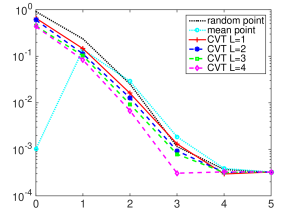
Table 1 gives the total CVT clustering energy of data set $X$ composed of 20000 samples. As the cluster number increases, the energy decreases gradually. The relative errors of quadrature test function approximated by the cut-HDMR expansions based on different anchors are listed in Table 2, and the results are visually shown in Figure 1. Although these approximation errors are almost equal when $r=5$ , they are different for lower order truncations. Obviously, it can not guarantee the accuracy of cut-HDMR expansion when the anchor is selected from parameter space randomly. Mean points with $r=0$ are well done for these two cases, because their zeroth-order terms are close to the expectations of function $u$ . Therefore, increasing the terms will lead to poor approximations until the expansions are sufficiently accurate. Note that the anchor point corresponding to $L=1$ in our model is close to the centroid of sparse grid proposed in [16], which is the center of input space $\bm{\Gamma}$ under uniform distribution. Compared with the above classical single anchor cut-HDMR expansions, our multiple anchors CVT-HDMR model can provide higher accuracy, and gradually improve with the increase of $L$ . This is consistent with the theoretical results described in section 3.2. The distance between input $\bm{\xi}$ and the anchor $\bar{\bm{\xi}}_{l}$ decreases with the increase of cluster number, resulting in smaller and smaller approximate errors.

Table 1: The total clustering energy

E_{\text{total}}

of 20000 input samples by the CVT method for different

L

and different distributions.

$L$	1	2	3	4
$E_{\text{total}}^{\text{Unif}}\times 10^{3}$	9.9845	8.7224	7.9745	7.3553
$E_{\text{total}}^{\text{Beta}}\times 10^{3}$	9.9722	8.7307	7.9489	7.3634

Table 2: The relative errors

\epsilon(\times 10^{-1})

of quadrature test function with different distributions computed using the cut-HDMR expansion for different anchors and truncation number

r

		Uniform					Standard beta
$r$		1	2	3	4	5	1	2	3	4	5
random point		1.6773	0.1725	0.0048	0.0027	0.0026	2.3651	0.2526	0.0115	0.0037	0.0032
mean point		0.2367	0.0174	0.0033	0.0026	0.0026	1.3908	0.2899	0.0186	0.0039	0.0032
CVT	$L=1$	0.2542	0.0158	0.0022	0.0026	0.0026	1.4592	0.1606	0.0131	0.0030	0.0033
	$L=2$	0.1835	0.0143	0.0022	0.0026	0.0026	1.1248	0.1273	0.0093	0.0032	0.0032
	$L=3$	0.2539	0.0108	0.0019	0.0026	0.0026	1.0249	0.0932	0.0079	0.0032	0.0032
	$L=4$	0.1935	0.0079	0.0025	0.0026	0.0026	0.8343	0.0677	0.0031	0.0033	0.0032

Refer to caption — Figure 1: The relative errors of quadrature test function computed using the cut-HDMR expansion with different anchors: (a) uniform distribution; (b) standard beta distribution.

4.2 Elliptic SPDE with Gaussian distributed variables

Next, using an elliptic SPDE with Gaussian distributed random variables to verify the effectiveness of our method.

\left\{\begin{array}[]{rll}-\nabla\cdot(a(\mathbf{x};\omega)\nabla u(\mathbf{x};\omega))&=\mathbf{f}(\mathbf{x}),&\quad\mathbf{x}\in D,\\ u(\mathbf{x};\omega)&=0,&\quad\mathbf{x}\in\partial D,\\ \end{array}\right.

(45)

where $D=[0,1]^{2}$ , source term $\mathbf{f}(\mathbf{x})$ is given by

\mathbf{f}(\mathbf{x})=4+\sin(2\pi x)\sin(4\pi y),

(46)

and diffusion function $a(\mathbf{x};\omega)$ satisfies

a(\mathbf{x};\omega)=\frac{1}{10}\exp\left(1.2\sum_{i=1}^{p}\sqrt{\lambda_{i}}\vartheta_{i}(\mathbf{x})\xi_{i}(\omega)\right).

(47)

Here, $\{\lambda_{i},\vartheta_{i}(\mathbf{x})\}$ is eigenpair of covariance function

Cov_{a}(\mathbf{x},\mathbf{x}^{\prime})=\exp\left(-\frac{\|\mathbf{x}-\mathbf{x}^{\prime}\|_{2}^{2}}{0.5}\right),

(48)

the dimension of random input $\bm{\xi}$ is $p=5$ , and parameter $\xi_{i}\sim\mathcal{N}(0,1)$ for $i=1,2,\ldots,p$ .

In our computation, the discrete solution $u$ is generated by the finite element method with mesh size $2^{-6}$ , i.e. $m=4225$ . The error measures are defined as

\mathcal{E}=\mathbb{E}\left[\frac{\|u(\bm{\xi})-\widehat{u}^{L,r}(\bm{\xi})\|_{2}^{2}}{\|u(\bm{\xi})\|_{2}^{2}}\right]\quad\text{ and }\quad\mathcal{V}=Var\left[\frac{\|u(\bm{\xi})-\widehat{u}^{L,r}(\bm{\xi})\|_{2}^{2}}{\|u(\bm{\xi})\|_{2}^{2}}\right],

(49)

where $\mathbb{E}[\cdot]$ and $Var[\cdot]$ denote the expectation and variance, respectively. These error statistics are estimated by the Monte Carlo method with 5000 samples. Here, the size of data set $X$ is set to $N=5000$ , the truncated order of HDMR expansion is $r=2$ , and the number of discrete points in each direction is equal to $K=7$ . Then $S_{K}=1+p(K-1)+\frac{p(p-1)(K-1)^{2}}{2}$ simulations are needed for constructing a cut-HDMR, and the total evaluations for building the CVT-HDMR is $S_{T}=LS_{K}$ . Therefore, there should not be too many anchors in our model for complex problems.

4.2.1 Construction of CVT-HDMR expansion

Table 3 lists the CVT clustering energy of data set $X$ composed of 5000 samples, which decreases with the increase of cluster number $L$ . Figure LABEL:eg2_F_C0 displays the diffusion functions associated with all CVT clustering centroids $\{\bar{\bm{\xi}}_{l}\}_{l=1}^{L}$ for different $L$ , and they have obvious differences. Table 4 gives the total number of simulations used for constructing the CVT-HDMR expansion. As $L$ increases, the sample size required to construct our model increases linearly. In our computational, the data needed for the single anchor cut-HDMR based on random point and mean point are consistent with $L=1$ in CVT-HDMR, both of which are 391. Note that the random input $\bm{\xi}$ satisfies Gaussian distribution, so the sparse grid centroid is equivalent to the center of parameter space $\bm{\Gamma}$ , and can be approximated by the anchor point of CVT-HDMR at $L=1$ .

Table 3: The total clustering energy

E_{\text{total}}

of set

X

by the CVT method for different

L

$L$	1	2	3	4
$E_{\text{total}}\times 10^{4}$	2.4713	2.1361	1.9083	1.7370

Table 4: The total number of simulations

S_{T}

for constructing the CVT-HDMR with different

L

and

K=7

$L$	1	2	3	4
$S_{T}$	391	782	1173	1564

4.2.2 Effectiveness of CVT-HDMR

In our calculations, the discrete point set is chosen in the entire parameter space $\bm{\Gamma}$ in order to compare with other models first. Table 5 lists the error estimate of traditional single anchor cut-HDMR based on each centroid $\bar{\bm{\xi}}_{l}$ , which is generated by CVT clustering method. The results show that the accuracy of cut-HDMR expansions obtained from different anchor points will vary greatly, which intuitively indicates the importance of anchor point location. In order to mitigate the negative effect of “poor” anchor, the multiple anchors model is proposed. Table 6 gives the error estimations of CVT-HDMR and Ave-HDMR under the same construction cost. Compared with the results in Table 5, the detrimental effects of improper anchors can be balanced by averaging several cut-HDMR expressions, but its accuracy does not exceed the best one among the selected anchors for a given $L$ . While our model have a significant improvement. The accuracy of CVT-HDMR increases with the increase of cluster number when $1\leq L\leq 3$ . It can be seen from the variances that the stability is also guaranteed. Although the errors corresponding to $L=4$ is slightly larger than that of $L=3$ , the results are acceptable. The main reasons for this phenomenon are that the data set $X$ is limited, and the sample points on the interfaces will increase with the increase of $L$ . Here, the multiple anchors models are also compared with the single anchor expansion based on the mean point. Clearly, the mean point is not appropriate as the anchor in this experiment. A realization of elliptic SPDE and its approximation errors associated with different methods and different $L$ are shown in Figures 3 and 4, respectively.

Table 5: Error estimates of single anchor cut-HDMR based on

\bar{\bm{\xi}}_{l}

for different

L

and

K=7

$L$	1	2		3			4
anchor	$\bar{\bm{\xi}}_{1}$	$\bar{\bm{\xi}}_{1}$	$\bar{\bm{\xi}}_{2}$	$\bar{\bm{\xi}}_{1}$	$\bar{\bm{\xi}}_{2}$	$\bar{\bm{\xi}}_{3}$	$\bar{\bm{\xi}}_{1}$	$\bar{\bm{\xi}}_{2}$	$\bar{\bm{\xi}}_{3}$	$\bar{\bm{\xi}}_{4}$
$\mathcal{E}\times 10^{-3}$	0.4870	1.6299	0.3636	1.9776	0.3002	1.6136	1.9376	0.3129	0.6407	2.6331
$\mathcal{V}\times 10^{-4}$	0.1000	0.9609	0.0645	1.5619	0.0198	1.2544	1.3267	0.0218	0.1750	3.0557

Table 6: Error estimates of single anchor cut-HDMR based on mean point, multiple anchors models CVT-HDMR and Ave-HDMR for different

L

and

K=7

	CVT-HDMR			Ave-HDMR			mean point
$L$	2	3	4	2	3	4	-
$\mathcal{E}\times 10^{-3}$	0.3760	0.2212	0.2426	0.6631	0.6427	0.6041	0.9913
$\mathcal{V}\times 10^{-4}$	0.0766	0.0197	0.0424	0.1715	0.1574	0.1374	0.3704

In order to compare with other methods in the above experiments, the discrete point set $\{Y_{i}^{l}\}_{i=1}^{p}$ used to construct the expansion $\widehat{f}^{(l,r)}(\bm{\xi})$ covers the whole parameter space $\bm{\Gamma}$ for $l=1,2,\ldots,L$ . But for our model, the points $\{Y_{i}^{l}\}_{i=1}^{p}$ only need to cover the Voronoi set $X_{l}$ . Table 7 gives the error estimates of the CVT-HDMR expansion, where $a_{i}$ and $b_{i}$ in point set $Y_{i}^{l}$ are the minimum and maximum values of the $i$ -th direction of set $X_{l}$ , respectively. Compared with Table 6, it can be observed that when the offline cost of model construction is equal, higher accuracy can be obtained by using the interpolation nodes covering the corresponding area since the interpolation error is reduced. This further verifies the proposed method is better than the Ave-HDMR expansion.

Table 7: Error estimates of CVT-HDMR, where discrete points cover the corresponding Voronoi set and

K=7

$L$	2	3	4
$\mathcal{E}\times 10^{-3}$	0.2627	0.1747	0.2022
$\mathcal{V}\times 10^{-4}$	0.0272	0.0095	0.0322

A single simulation of elliptic SPDE (45) using the finite element method with mesh size $h=2^{-6}$ takes 0.6082 seconds, while our CVT-HDMR expansion takes only 0.1132 seconds to obtain an accurate approximation of the response. The construction of HDMR in the offline stage is expensive, but it can be balanced by the fast calculation in online stage. Therefore, this method can be used for problems that require a lot of repeated calculations.

5 Conclusions

Based on the CVT clustering method, we provide a construction strategy for the multiple anchors cut-HDMR expansion, which applies the centroids as the anchors to establish the corresponding expansions, and then uses the nearest principle to generate the approximate response of the given input. Numerical experiments show that the CVT-HDMR method is more accurate and stable than the single anchor model and the average of several cut-HDMR expansions. However, with the increase of the cluster number $L$ , the construction cost of the CVT-HDMR increases linearly, and the number of samples on the interface also increases, which affects the accuracy of the CVT-HDMR expansion. Therefore, it is necessary to study the appropriate cluster number for this multiple anchors model. In addition, the specific application of the CVT-HDMR expansion is also a subject worth studying in the future.

References

[1] Li, G., Rosenthal, C., and Rabitz, H., High dimensional model representations, J. Phys. Chem. A, 105(33), 2001.
[2] Rabitz, H. and Aliş, Ö.F., General foundations of high-dimensional model representations, J. Math. Chem., 25(2):197–233, 1999.
[3] Sobol’, I.M., Sensitivity estimates for nonlinear mathematical models, Math. Modeling Comput. Experiment, 1(4):407–414 (1995), 1993.
[4] Cao, Y., Chen, Z., and Gunzburger, M., ANOVA expansions and efficient sampling methods for parameter dependent nonlinear PDEs., Int. J. Numer. Anal. Model., 6(2):256–273, 2009.
[5] Rabitz, H., Aliş, Ö.F., Shorter, J., and Shim, K., Efficient input-output model representations, Comput. Phys. Commun., 117(1-2):11–20, 1999.
[6] Smith, R.C., Uncertainty Quantification: Theory, Implementation, and Applications, Vol. 12, SIAM, 2013.
[7] Sobol’, I.M., Theorems and examples on high dimensional model representation, Reliab. Eng. Syst. Saf., 79(2):187–193, 2003.
[8] Wang, X., On the approximation error in high dimensional model representation, In 2008 Winter Simulation Conference, pp. 453–462. IEEE, 2008.
[9] Cheng, K., Lu, Z., Ling, C., and Zhou, S., Surrogate-assisted global sensitivity analysis: an overview, Struct. Multidiscip. Optim., 61(3):1187–1213, 2020.
[10] Chowdhury, R., Rao, B., and Prasad, A.M., High-dimensional model representation for structural reliability analysis, Commun. Numer. Methods Eng., 25(4):301–337, 2009.
[11] Chowdhury, R. and Rao, B., Hybrid high dimensional model representation for reliability analysis, Comput. Meth. Appl. Mech. Eng., 198(5-8):753–765, 2009.
[12] Huang, H., Wang, H., Gu, J., and Wu, Y., High-dimensional model representation-based global sensitivity analysis and the design of a novel thermal management system for lithium-ion batteries, Energy Conv. Manag., 190:54–72, 2019.
[13] Kubicek, M., Minisci, E., and Cisternino, M., High dimensional sensitivity analysis using surrogate modeling and high dimensional model representation, Int. J. Uncertain. Quantif., 5(5), 2015.
[14] Li, D., Tang, H., Xue, S., and Guo, X., Reliability analysis of nonlinear dynamic system with epistemic uncertainties using hybrid Kriging-HDMR, Probab. Eng. Mech., 58:103001, 2019.
[15] Wang, H., Chen, L., Ye, F., and Chen, L., Global sensitivity analysis for fiber reinforced composite fiber path based on D-MORPH-HDMR algorithm, Struct. Multidiscip. Optim., 56(3):697–712, 2017.
[16] Gao, Z. and Hesthaven, J.S., On ANOVA expansions and strategies for choosing the anchor point, Appl. Math. Comput., 217(7):3274–3285, 2010.
[17] Yue, X., Zhang, J., Gong, W., Luo, M., and Duan, L., An adaptive PCE-HDMR metamodeling approach for high-dimensional problems, Struct. Multidiscip. Optim., 64(1):141–162, 2021.
[18] Li, G., Wang, S.W., and Rabitz, H., Practical approaches to construct RS-HDMR component functions, J. Phys. Chem. A, 106(37):8721–8733, 2002.
[19] Li, G., Hu, J., Wang, S.W., Georgopoulos, P.G., Schoendorf, J., and Rabitz, H., Random sampling-high dimensional model representation (RS-HDMR) and orthogonality of its different order component functions, J. Phys. Chem. A, 110(7):2474–2485, 2006.
[20] Mukhopadhyay, T., Dey, T., Chowdhury, R., Chakrabarti, A., and Adhikari, S., Optimum design of FRP bridge deck: an efficient RS-HDMR based approach, Struct. Multidiscip. Optim., 52(3):459–477, 2015.
[21] Zhang, Z., Choi, M., and Karniadakis, G.E. Anchor points matter in ANOVA decomposition. In Spectral and High Order Methods for Partial Differential Equations, pp. 347–355. Springer, 2011.
[22] Labovsky, A. and Gunzburger, M., An efficient and accurate method for the identification of the most influential random parameters appearing in the input data for PDEs, SIAM-ASA J. Uncertain. Quantif., 2(1):82–105, 2014.
[23] Shan, S. and Wang, G.G., Metamodeling for high dimensional simulation-based design problems, J. Mech. Des., 132(5), 2010.
[24] Cai, X., Qiu, H., Gao, L., Yang, P., and Shao, X., An enhanced RBF-HDMR integrated with an adaptive sampling method for approximating high dimensional problems in engineering design, Struct. Multidiscip. Optim., 53(6):1209–1229, 2016.
[25] Liu, H., Hervas, J.R., Ong, Y.S., Cai, J., and Wang, Y., An adaptive RBF-HDMR modeling approach under limited computational budget, Struct. Multidiscip. Optim., 57(3):1233–1250, 2018.
[26] Anand, V., Patnaik, B.S.V., and Rao, B.N., Efficient Extraction of Vortex Structures by Coupling Proper Orthogonal Decomposition (POD) and High–Dimensional Model Representation (HDMR) Techniques, Numer Heat Tranf. B-Fundam., 61(3):229–257, 2012.
[27] Tang, L., Wang, H., and Li, G., Advanced high strength steel springback optimization by projection-based heuristic global search algorithm, Mater. Des., 43:426–437, 2013.
[28] Ji, L., Chen, G., Qian, L., Ma, J., and Tang, J., An iterative interval analysis method based on Kriging-HDMR for uncertainty problems, Acta Mech. Sin., 38(7):1–13, 2022.
[29] Chen, L., Li, E., and Wang, H., Time-based reflow soldering optimization by using adaptive Kriging-HDMR method, Solder. Surf. Mt. Technol., 28(2):101–113, 2016.
[30] Li, E. and Wang, H., An alternative adaptive differential evolutionary algorithm assisted by expected improvement criterion and cut-HDMR expansion and its application in time-based sheet forming design, Adv. Eng. Softw., 97:96–107, 2016.
[31] Li, E., Ye, F., and Wang, H., Alternative Kriging-HDMR optimization method with expected improvement sampling strategy, Eng. Comput., 2017.
[32] Hajikolaei, K.H. and Gary Wang, G., High dimensional model representation with principal component analysis, J. Mech. Des., 136(1):011003, 2014.
[33] Haji Hajikolaei, K., Cheng, G.H., and Wang, G.G., Optimization on metamodeling-supported iterative decomposition, J. Mech. Des., 138(2):021401, 2016.
[34] Huang, Z., Qiu, H., Zhao, M., Cai, X., and Gao, L., An adaptive SVR-HDMR model for approximating high dimensional problems, Eng. Comput., 32(3):643–667, 2015.
[35] Li, G., Xing, X., Welsh, W., and Rabitz, H., High dimensional model representation constructed by support vector regression. I. Independent variables with known probability distributions, J. Math. Chem, 55(1):278–303, 2017.
[36] Ren, O., Boussaidi, M.A., Voytsekhovsky, D., Ihara, M., and Manzhos, S., Random sampling high dimensional model representation gaussian process regression (RS-HDMR-GPR) for representing multidimensional functions with machine-learned lower-dimensional terms allowing insight with a general method, Comput. Phys. Commun., 271:108220, 2022.
[37] Chen, L., Wang, H., Ye, F., and Hu, W., Comparative study of HDMRs and other popular metamodeling techniques for high dimensional problems, Struct. Multidiscip. Optim., 59(1):21–42, 2019.
[38] Chen, L., Wang, H., Fan, Y., and Hu, W., Correction to: Comparative study of HDMRs and other popular metamodeling techniques for high dimensional problems, Struct. Multidiscip. Optim., 61(1):433–435, 2020.
[39] Baran, M. and Bieniasz, L.K., Experiments with an adaptive multicut-HDMR map generation for slowly varying continuous multivariate functions, Appl. Math. Comput., 258:206–219, 2015.
[40] Li, G., Schoendorf, J., Ho, T.S., and Rabitz, H., Multicut-hdmr with an application to an ionospheric model, J. Comput. Chem., 25(9):1149–1156, 2004.
[41] Du, Q., Faber, V., and Gunzburger, M., Centroidal Voronoi tessellations: Applications and algorithms, SIAM Rev., 41(4):637–676, 1999.
[42] Du, Q., Emelianenko, M., and Ju, L., Convergence of the Lloyd algorithm for computing centroidal Voronoi tessellations, SIAM J. Numer. Anal., 44(1):102–119, 2006.
[43] Burkardt, J., Gunzburger, M., and Lee, H.C., Centroidal Voronoi tessellation-based reduced-order modeling of complex systems, SIAM J. Sci. Comput., 28(2):459–484, 2006.
[44] Karcılı, A. and Tunga, B., Content based image retrieval using HDMR constant term based clustering, In International Conference on Mathematics and its Applications in Science and Engineering, pp. 35–45. Springer, 2022.
[45] Davis, P.J., Interpolation and approximation, Courier Corporation, 1975.
[46] Lloyd, S., Least squares quantization in PCM, IEEE Trans. Inf. Theory, 28(2):129–137, 1982.
[47] MacQueen, J., Some methods for classification and analysis of multivariate observations, In Proc. Fifth Berkeley Sympos. Math. Statist. and Probability (Berkeley, Calif., 1965/66), Vol. I: Statistics, pp. 281–297. Univ. California Press, Berkeley, Calif., 1967.
[48] Heiss, F. and Winschel, V., Likelihood approximation by numerical integration on sparse grids, J. Econom., 144(1):62–80, 2008.
[49] Patterson, T.N., The optimum addition of points to quadrature formulae, Math. Comput., 22(104):847–856, 1968.
[50] Petras, K., Smolyak cubature of given polynomial degree with few nodes for increasing dimension, Numer. Math., 93(4):729–753, 2003.