sublue \addauthorcymagenta \addauthornkred
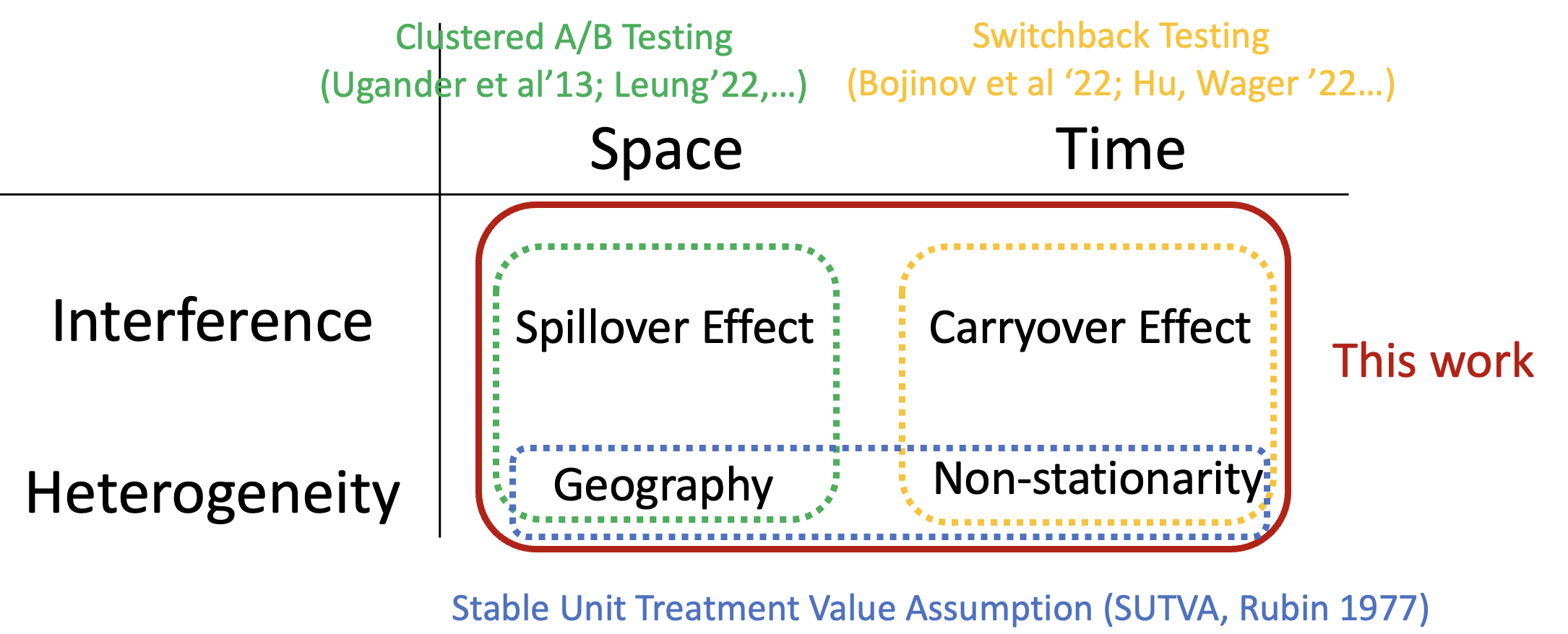
Clustered Switchback Designs for
Experimentation Under Spatio-temporal Interference
Abstract
We consider experimentation in the presence of non-stationarity, inter-unit (spatial) interference, and carry-over effects (temporal interference), where we wish to estimate the global average treatment effect (GATE), the difference between average outcomes having exposed all units at all times to treatment or to control. We suppose spatial interference is described by a graph, where a unit’s outcome depends on its neighborhood’s treatments, and that temporal interference is described by an MDP, where the transition kernel under either treatment (action) satisfies a rapid mixing condition. We propose a clustered switchback design, where units are grouped into clusters and time steps are grouped into blocks, and each whole cluster-block combination is assigned a single random treatment. Under this design, we show that for graphs that admit good clustering, a truncated Horvitz-Thompson estimator achieves a mean squared error (MSE), matching the lower bound up to logarithmic terms for sparse graphs. Our results simultaneously generalize the results from Hu and Wager (2022); Ugander et al. (2013) and Leung (2022). Simulation studies validate the favorable performance of our approach.
1 Introduction
| Prior Work | #individuals | #rounds | Interference Graph | Clustering | MSE |
|---|---|---|---|---|---|
| Hu and Wager (2022) | singleton | n/a | |||
| Ugander and Yin (2023) | -restricted growth graphs | -net | |||
| Leung (2022) | Intersection graph of balls | uniform |
Randomized experimentation, or A/B testing, is \cyreplacea broadly deployed learning tool in online commerce that is simple to execute.widely used to estimate causal effects on online platforms. Basic strategies involve partitioning the experimental units (e.g., individuals or time periods) into two groups randomly, and assigning one group to treatment and the other to control. A key challenge in modern A/B testing is interference: From two-sided markets to social networks, interference between individuals complicates experimentation and makes it difficult to estimate the true effect of a treatment.
The spillover effect in experimentation has been extensively studied (Manski, 2013; Aronow et al., 2017; Li et al., 2021; Ugander et al., 2013; Sussman and Airoldi, 2017; Toulis and Kao, 2013; Basse and Airoldi, 2018; Cai et al., 2015; Gui et al., 2015; Eckles et al., 2017a; Chin, 2019). Most of these works assume \cyeditneighborhood interference, where the spillover effect is \cyeditconstrained to the direct neighborhood of an individual as given by an interference graph. Under this assumption, Ugander et al. (2013) proposed a clustering-based design, and showed that if the growth rate of neighborhoods is bounded, then the Horvitz-Thompson (HT) estimator achieves a mean squared error (MSE) of where is the maximum degree. Later, Ugander and Yin (2023) showed that by introducing randomness into the clustering, the dependence on can be improved to polynomial. \cyreplaceAnother example is spatial interference. Leung (2022) considered the geometric graph induced by an almost uniformly spaced point set in the plane and assumed that the level of interference between two individuals decays with their (spatial) distance.As there are many settings in which interference extends beyond direct neighbors, Leung (2022) considers a relaxed assumption in which the interference is not restricted to direct neighbors, but decays as a function of the spatial distance between individuals with respect to an embedding of the individuals in Euclidean space.
Orthogonal to the spillover effect, the carryover effect (or temporal interference), where past treatments may affect future outcomes, has also been extensively studied. Bojinov et al. (2023) considers \cyedita simple model in which the temporal interference \cyeditis bounded by a fixed window length. Other works model temporal interference that arises from the Markovian evolution of states, \cyeditwhich allows for interference effects that can persist across long time horizons (Glynn et al., 2020; Farias et al., 2022; Hu and Wager, 2022; Johari et al., 2022; Shi et al., 2023). A \cyeditcommonly used approach in practice is to deploy switchback experiments: The exposure of the entire system (viewed as a single experimental unit) \cyreplaceto a single treatment at a time, interchangeably switching the treatment between the two options over interspersed blocks of time.alternates randomly between treatment and control for sufficiently long contiguous blocks of time such that the temporal interference around the switching points does not dominate. \cydeleteMoreover, despite the literature on Markovian switchback models, the minimax MSE rate for the case remains unknown. \cyeditUnder a switchback design, Hu and Wager (2022) showed that a MSE rate can be achieved, assuming that the Markov chains have mixing time .
While the prior studies either focused on only network interference or only temporal interference, there are many practical settings in which both types of interference are present, such as online platforms, healthcare systems, or ride-sharing networks. In these environments, an individual’s outcome may depend not only on who else is treated nearby but also on how the individual’s “state” has evolved over time, making it essential to develop methodologies that can handle both dimensions jointly.
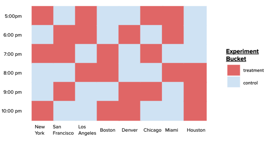
To address this, clustered switchback experiments have become widely adopted in industry. The idea is to partition both the space (e.g., by geographics or a social network) and time into discrete blocks, and then randomize at the level of space-time clusters (i.e., product set of spatial and temporal blocks). For example, DoorDash randomizes promotions at the region-hour level (see Fig. 1). This allows practitioners to mitigate interference within clusters while preserving statistical power and operational feasibility.
Despite its practical popularity, the theoretical foundations of this approach remain underexplored. On the surface, handling spatio-temporal interference seems straightforward, considering that (i) time can be regarded as an additional “dimension”, and (ii) these two types of interference have been well explored separately. However, in most work on network interference, the potential outcomes \cyeditconditioned on the treatment assignments are assumed to be independent (e.g., Ugander et al. (2013); Leung (2022)). In a Markovian setting, this assumption breaks down, since \cyreplacepast treatments may affect future outcomes throughpast outcomes are correlated to future outcomes even conditioned on the treatments due to state evolution.
We consider experimentation with spatio-temporal interference on a model that encapsulates both (i) the network interference between individuals by a given interference graph, and (ii) the temporal interference \cyreplaceby associating a state to each individual that evolves in a Markovian fashion independently.that arises from Markovian state evolutions. We assume that the outcome and state evolution of each individual depends solely on the treatments of their immediate neighborhood (including themselves), \cyeditand that the state evolutions are independent across individuals conditioned on the treatments.
1.1 Our Contributions
Our main theorem states that a truncated HT estimator achieves an MSE of times a \cyreplacesome combinatorial parameters that involve and the interference graph ; see Theorem 1.graph clustering-dependent quantity which is for low-degree graphs for good clusterings, e.g., growth restricted graphs (Ugander et al., 2013) or spatially derived graphs (Leung, 2022). This result bridges the literature on experimentation with spatial/network interference and temporal interference by extending the following results:
- 1.
-
2.
Network interference. Assuming that the interference graph satisfies the -restricted growth condition (defined in Section 4), Ugander et al. (2013) showed that the HT estimator achieves an MSE of for with a suitable partition (graph clustering), where is the maximum degree. Moreover, by introducing randomness into the clustering, Ugander and Yin (2023) improved the exponential dependence on to polynomial, achieving a MSE. Our Corollary 4 generalizes this to in the presence of Markovian temporal interference.
| Interference Graph | (Spatio-) Clustering | MSE | Reference |
|---|---|---|---|
| No edges (i.e., no interference) | one node per cluster | Corollary 1 | |
| Singleton (i.e., pure switchback) | n/a | Corollary 2 | |
| Maximum Degree | arbitrary | Corollary 3 | |
| -Restricted Growth | -hop-random | Corollary 4 | |
| Intersection graph of radius- balls | uniform | Corollary 5 |
We state our results under the -fractional neighborhood exposure (-FNE) as introduced in Ugander et al. (2013); Eckles et al. (2017b), generalizing beyond the “exact” (i.e., ) neighborhood interference assumption. We summarize our results (with for simplicity) in Table 2.
We emphasize that our setting, even for , can not be reduced to that of Leung 2022. Essentially, this is because their independence assumptions no longer holds here. We will provide more details in a dedicated discussion section Section 3.2.
1.2 Related Work
Violation of SUTVA. Experimentation is a broadly deployed learning tool in e-commerce that is simple to execute (Kohavi and Thomke, 2017; Thomke, 2020; Larsen et al., 2023). As a key challenge, the violation of the so-called Stable Unit Treatment Value Assumption (SUTVA) has been viewed as problematic in online platforms (Blake and Coey, 2014).
Many existing works that tackle this problem assume that interference is summarized by a low-dimensional exposure mapping and that individuals are individually randomized into treatment or control by Bernoulli randomization (Manski, 2013; Toulis and Kao, 2013; Aronow et al., 2017; Basse et al., 2019; Forastiere et al., 2021). Some work departed from unit-level randomization and introduced cluster dependence in unit-level assignments in order to improve estimator precision, including Ugander et al. 2013; Jagadeesan et al. 2020; Leung 2022, 2023, just to name a few.
There is another line of work that considers the temporal interference (or carryover effect). Some works consider a fixed bound on the persistence of temporal interference (e.g., Bojinov et al. (2023)), while other works considered temporal interference arising from the Markovian evolution of states (Glynn et al., 2020; Farias et al., 2022; Johari et al., 2022; Shi et al., 2023; Hu and Wager, 2022; Li and Wager, 2022; Li et al., 2023). Apart from being limited to the single-individual setting, many of these works differ from ours either by (i) focusing on alternative objectives, such as stationary outcome Glynn et al. (2020), or (ii) imposing additional assumptions, like observability of the states Farias et al. (2022).
Spatio-temporal Interference. Although extensively studied separately and recognized for its practical significance, experimentation under spatio-temporal interference has received relatively limited attention previously. Recently, Ni et al. (2023) attempted to address this problem, but their carryover effect is confined to one period. \cydeletesee their Assumption 2. Another closely related work is Li and Wager 2022. Similar to our work, they specified the spatial interference using an interference graph and modeled temporal interference by assigning an MDP to each individual. In our model, the transition probability depends on the states of all neighbors (in the interference graph). In contrast, their evolution depends on the sum of the outcome of direct neighbors. Moreover, our work focuses on ATE estimation for a fixed, unknown environment, whereas they focus on the large sample asymptotics and mean-field properties. Wang (2021) studied direct treatment effects for panel data under spatiotemporal interference, but focused on asymptotic properties instead of finite-sample bounds.
Off-Policy Evaluation (OPE) Since we model temporal interference using an MDP, our work is naturally related to reinforcement learning (RL). In fact, our result on ATE estimation can be rephrased as OPE (Jiang and Li, 2016; Thomas and Brunskill, 2016) in a multi-agent MDP: Given a behavioral policy from which the data is generated, we aim to evaluate the mean reward of a target policy. The ATE in our work is essentially the difference in the mean reward between two target policies (all-1 and all-0 policies), and the behavioral policy is given by clustered randomization. However, these works usually require certain states to be observable, which is not needed in our work. Moreover, these works usually impose certain assumptions on the non-stationarity, which we allow to be completely arbitrary. Finally, we focus on rather general data-generating policies (beyond fixed-treatment policies) and estimands (beyond ATE), compromising the strengths of the results.
2 Model Setup and Experiment Design
2.1 Formulation
Consider a horizon with rounds and individuals, where each individual is randomly assigned to treatment (“1”) or control (“0”) at each time. We model the interference between individuals using an interference graph where and each node represents an individual. Formally, the treatment assignment is given by a binary matrix . \cydeleteAlthough it may sometimes be reasonable to assign the treatments in each round adaptively, We focus on non-adaptive designs where is drawn at the beginning and hence is independent of all other variables, including the individuals’ states and outcomes.
To model temporal interference, we assign each individual a state at time that evolves independently in a Markovian fashion. The transition kernel is a function of the treatments of and its direct neighbors in at time , which we refer to as the \cyeditinterference neighborhood of , denoted . The state at time , , is drawn from a distribution . We allow to vary arbitrarily across different combinations of and .
An observed outcome is generated as a function of (i) the unit’s state and (ii) the treatments of itself and its neighbors, according to
where has mean zero. The \cyeditconditional mean outcome is determined by , which we call the outcome function. The model dynamics are thus specified by the sequence
We emphasize that we do not assume observation of the state variables.
Given the observations (consisting solely of ), our objective is to estimate the difference between the \cyeditcounterfactual outcomes under continuous deployment of treatment and treatment , averaged over all individuals and rounds, referred to as the Global Average Treatment Effect.
Definition 1 (Global Average Treatment Effect).
Let be any distribution over , and denote by . The global average treatment effect (GATE) is
If the Markov chains are rapid-mixing (defined soon), then “matters” only by a lower-order term compared to the MSE (see Proposition 1), and we will thus suppress . We also want to point out that our results still hold if “” and “” are replaced with an arbitrary pair of fixed treatment sequences.
2.2 Assumptions
A key assumption as introduced in Hu and Wager (2022) that allows for estimation despite temporal interference is rapid mixing:
Assumption 1 (Rapid Mixing).
There exists a constant such that for any , , and distributions over , we have
As a convenient consequence, the initial state distribution does not matter much.
Proposition 1 (Initial State Doesn’t Matter).
For any distributions over , we have
| (1) |
Consequently,
The above implies that the error caused by misspecifying the initial distribution is , and thus it contributes only a term to the MSE. This is of lower order compared to our MSE bound, which scales as , as we will soon see.
We assume that the mean-zero noise \cyreplaceindependenthave zero cross-correlation and bounded \cyreplacecorrelationvariance:
Assumption 2 (Uncorrelated Noise).
Write . There is a constant s.t. for all , , we have
We state our results under the -Fractional Neighborhood Exposure (-FNE) mapping as introduced in Ugander et al. (2013); Eckles et al. (2017a); the neighborhood interference assumption is the special case when . For concreteness, the reader may assume without losing sight of the main ideas.
Assumption 3 (-FNE).
For any and s.t. , we have
2.3 Design and Estimator
We focus on \cyeditclustered switchback designs, which specify a distribution for sampling the treatment vector given a fixed clustering over the network.
Definition 2 (Clusters).
A family of subsets of is a clustering (or partition) if and for any . Each set is called a cluster.
We independently assign treatments to the cluster-timeblock product sets uniformly.
Definition 3 (Clustered Switchback Design).
Let be a clustering for . Uniformly partition into timeblocks of length (except the last one). For each block and , draw independently. Set for .
We consider a class of Horvitz-Thompson (HT) Horvitz and Thompson (1952) style estimators under a misspecified radius- exposure mapping, similar to that of Aronow et al. (2017); Leung (2022); Sävje (2024).
Definition 4 (Radius- Truncated Horvitz-Thompson (HT) Estimator).
For any radius , define the radius- truncated exposure mapping as
for any and . Define the exposure probability as
Denote
for , and . The Radius- Truncated Horvitz-Thompson estimator is given by
Note that as in previous literature, and are not independent, as they both depend on the treatments in the rounds before . The truncated HT estimator was proposed in the spatial interference setting (Leung, 2022), and utilizes the framework of misspecified exposure mappings introduced by Aronow et al. (2017); Sävje (2023).
Remark 1.
The radius- truncated exposure mapping is misspecified in the time dimension, since the treatments from could still impact the outcome at time through the correlation of the state distributions. The “true exposure mapping” is instead
However, the associated true exposure probability is exponentially low in , and thus by truncating the neighborhood in the time dimension, the misspecified exposure mapping enjoys a much higher exposure probability. This leads to a natural bias-variance tradeoff in the performance of the truncated Horvitz-Thompson estimator with respect to the choice of . Moreover, it serves as a good approximation of , as the rapid-mixing property implies that the correlation across long time scales is weak, and thus limits the impact that treatments from a long time ago can have on the current outcome.∎
2.4 Dependence Graph
The following will be useful when stating our results in the general form.
Definition 5 (Dependence Graph).
Given a partition of , the dependence graph is where for any (possibly identical), we include an edge in (and denote ) if there is a cluster s.t. and
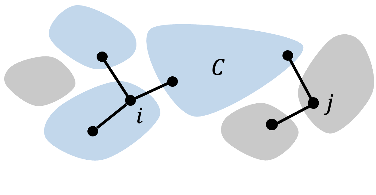
The reader should not confuse dependence graph with interference graph. The former is, in fact, always a supergraph of the latter. For example, if each cluster in is a singleton, then the dependence graph is the second power of the interference graph.
The dependence graph has the following useful property: If , then do not intersect any common cluster, and hence their outcomes and exposure mappings are independent.
Lemma 1 (Independence for Far-apart Individuals).
Fix a partition and . Suppose and . Then, for any , we have .
This result is the consequence of the following facts: (1) only depends on the treatments of the clusters that intersect , (2) implies where denotes the collection of clusters that intersects, and (3) the treatments are independently assigned to each cluster.
3 Main Results
3.1 MSE Upper Bound
Proposition 2 (Bias of the HT estimator).
For any , we have
The is reminiscent of the decaying interference assumption in Leung 2022 (albeit on distributions rather than realizations), which inspires us to consider a truncated HT estimator as considered therein. However, their analysis is not readily applicable to our Markovian setting, since their potential outcomes are deterministic.
Definition 6 (Cluster Degree).
Given a clustering of , for each we define
Recall that if where is the set of edges of the independence graph induced by .
Proposition 3 (Variance of the HT estimator).
Fix a clustering of and any . Denote Then,
In Section 4 we will further simplify the above by considering natural classes of graphs.
Taken together, we deduce that for any fixed , we have:
Theorem 1 (MSE Upper Bound).
Suppose , then
We will soon see that for “sparse” graphs or geometric graphs, the summation becomes , and thus the MSE becomes .
3.2 Discussions
We address some questions that the readers may have at this point.
1. Can we reduce to Leung (2022)? We emphasize that our Theorem 1 is not implied by Leung 2022. While the rapid mixing property implies that the temporal interference decays exponentially across time, which seems to align with Assumption 3 from Leung 2022, they critically assume that
which does not hold in our setting - the outcomes in our Markovian setting are not independent (albeit having weak covariance) over time, even conditioned on treatment assignment.
2. Comparison with Hu and Wager (2022). Independently, Hu and Wager (2022) obtained a MSE for , using a bias-corrected estimator which is similar to our HT estimator with . Our analysis is more general as it handles cases where . This is a significant distinction since, in practice, the block length is “externally” chosen, say, by an online platform, government, or nature, e.g., or .
Proposition 3 provides insights on how to select the best specific to this . For example, consider and . Then, Propositions 2 and 3 combined lead to an MSE of if
3.3 Practical Concern: Small Exposure Probability.
So far, we have stated our Theorem 1 in terms of the minimal exposure probabilities . Intuitively, smaller values of these probabilities lead to higher variance and worse MSE bounds. We next present lower bounds on these probabilities in (as in the -FNE, see 3).
Proposition 4 (Lower Bound of Exposure Probabilities).
Denote the entropy function . Then,
To see the intuition, consider and . For simplicity, assume that all clusters intersecting have the same cardinality. Then, the exposure mapping equals if at least of these clusters are assigned . Thus, the exposure probability is
Therefore, there is a probability (multiplying by two to account for both and ) that we will keep each data point. More generally, by Stirling’s formula, for any s.t. is an integer,
It follows that
Remark 2.
It is straightforward to verify that with (i.e., “exact” neighborhood condition), we have
for each . In particular, if , the above becomes . However, this probability may be too low to be considered practical. For example, if for most units , we will use only of the data. Proposition 4 improves the exposure probability (for ) due to the term in the exponent.
4 Implications on Special Clusterings
Let us simplify Theorem 1 for specific clusterings. Unless stated otherwise, we take and to highlight the key parameters.
Corollary 1 (No Interference).
Suppose the interference graph has no edge. Then, for the clustering , where each cluster is a singleton set, and , we have
The following holds for any interference graph.
Corollary 2 (Pure Switchback).
Consider the clustering where all individuals are in one cluster. For , we have
Remark 3.
As we recall from Definition 3, our block-based randomized design coincides with the switchback design in Hu and Wager 2022 when : Partition the time horizon into blocks and assign a random treatment independently to each block. \cydeletethroughout to each vertex independently. Hu and Wager (2022) analyzed aWhen , our model and design coincide with Hu and Wager 2022. They focus on a class of difference-in-mean (DIM) estimators which compute the difference in average outcomes between blocks assigned to treatment vs control, ignoring data from time points that are too close to the boundary (referred to as the burn-in period\cydelete and denoted ). While they show that the vanilla DIM estimators are limited to an MSE of , our results show that the truncated Horvitz-Thompson estimator obtains the optimal MSE, \cyeditmatching the improved rate of their concurrent bias-corrected estimator.∎
Now, we consider graphs with bounded degree.
Corollary 3 (Bounded-degree Graphs).
Let be the maximum degree of . Then, for the partition and ,
The above bound has an unfavorable exponential dependence in . This motivated Ugander et al. (2013) to introduce the following condition which assumes that the number of -hop neighbors of each node is dominated by a geometric sequence with a common ratio . Denote by the hop distance.
Definition 7 (Restricted Growth Coefficient).
A graph has a restricted growth coefficient (RGC) of , if
Example. An -spider graph consists of a root node attached to paths, each of length . Then, the graph has an RGC of . Another example is a social network that is globally sparse but locally dense. ∎
Ugander and Yin (2023) showed that in a -RGC graph, under their randomized group cluster randomization (RGCR), the exposure probability of each unit is at least for (see their Theorem 4.2). As a result, the MSE of the HT estimator is polynomial in and . By considering the product of their pure-spatio design and a uniform partition of the time horizon, it is straightforward to generalize their result as:
Theorem 2 (Ugander and Yin (2023), Generalized).
Using a 1-hop-max random clustering on a -RGC graph, then for any and , we have
Combining with Theorem 1, we obtain the following.
Corollary 4 (Restricted-Growth Graphs).
Suppose satisfies the -RGC and has maximum degree . Then, using the 1-hop-max random clustering in Ugander and Yin (2023), with , we have
Remark 4.
When , this matches Theorem 4.7 of Ugander and Yin 2023. Moreover, the above is stronger than Corollary 3 if . For example, for the spider graph, we have , so the MSE improves exponentially in . ∎
Now we consider spatially derived graphs. Suppose that the units are embedded into a lattice. We assume that the transitions and outcomes at a node can interfere with nodes within a hop distance . In other words, we include an edge in the interference graph if .
We achieve a MSE as follows. Consider a natural clustering. For any , we denote by the uniform partition of the lattice into square-shaped clusters of size . Then:
Corollary 5 (-neighborhood Interference).
For , we have for any . Consequently, with and ,
To complement the above, we want to point out that it is not hard to show the following lower bound:
Theorem 3 (MSE Lower Bound).
For any , if the interference graph has no edges, then for any estimator under any (possibly adaptive) design.
While this shows that the dependence on is optimal, this lower bound unfortunately does not suggest what the optimal dependence on the problem dependent parameters is. It would be of value for future study to consider whether one could obtain tighter lower bounds that indicate the optimal dependence on the properties of the spatial and temporal interference.
5 Simulation Study
5.1 Single-unit Setting ()
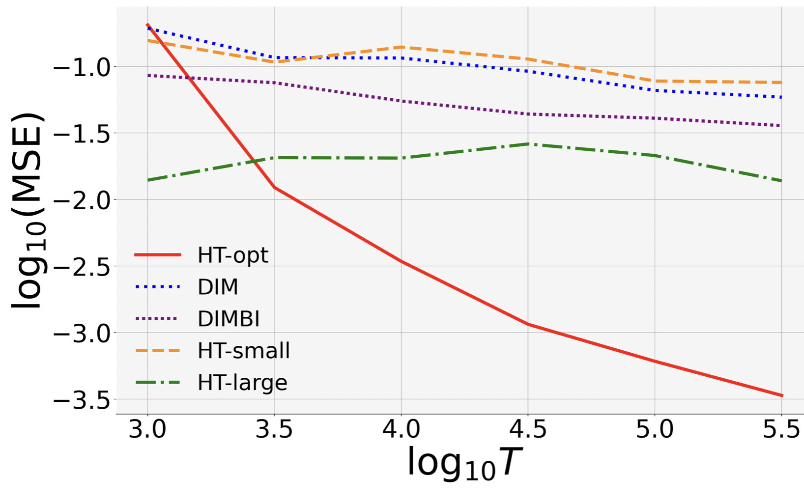
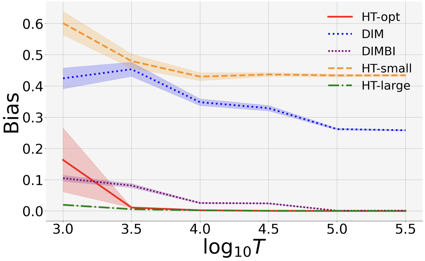
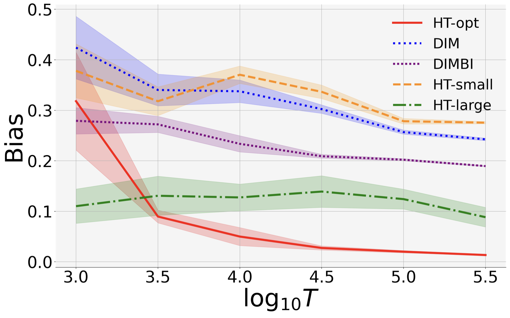
Our Theorem 1 states that the optimal MSE rate is achieved when the block length and HT radius are both . We next show the efficacy of this design-estimator combination through experiments.
Our MDP. The state evolves according to a clipped random walk with a stationary transition kernel. Specifically, the states are integers with an absolute value of at most . If we select treatment , we flip a coin with heads probability , and move up and down by one unit correspondingly, except at “boundary states” , where we stay put if the coin toss informs us to move outside. The reward function is non-stationary over time and depends only on the state. Specifically, letting be two sequences of real numbers, we define for each , and .
The DIMBI estimator. We will compare with the Difference-In-Means with Burn-In (DIMBI) estimator in Hu and Wager (2022), which discards the first (“burn-in”) observations in each block and calculates the difference in the mean outcomes in the remaining observations. Formally, let be the block length and be a treatment vector, for each we define
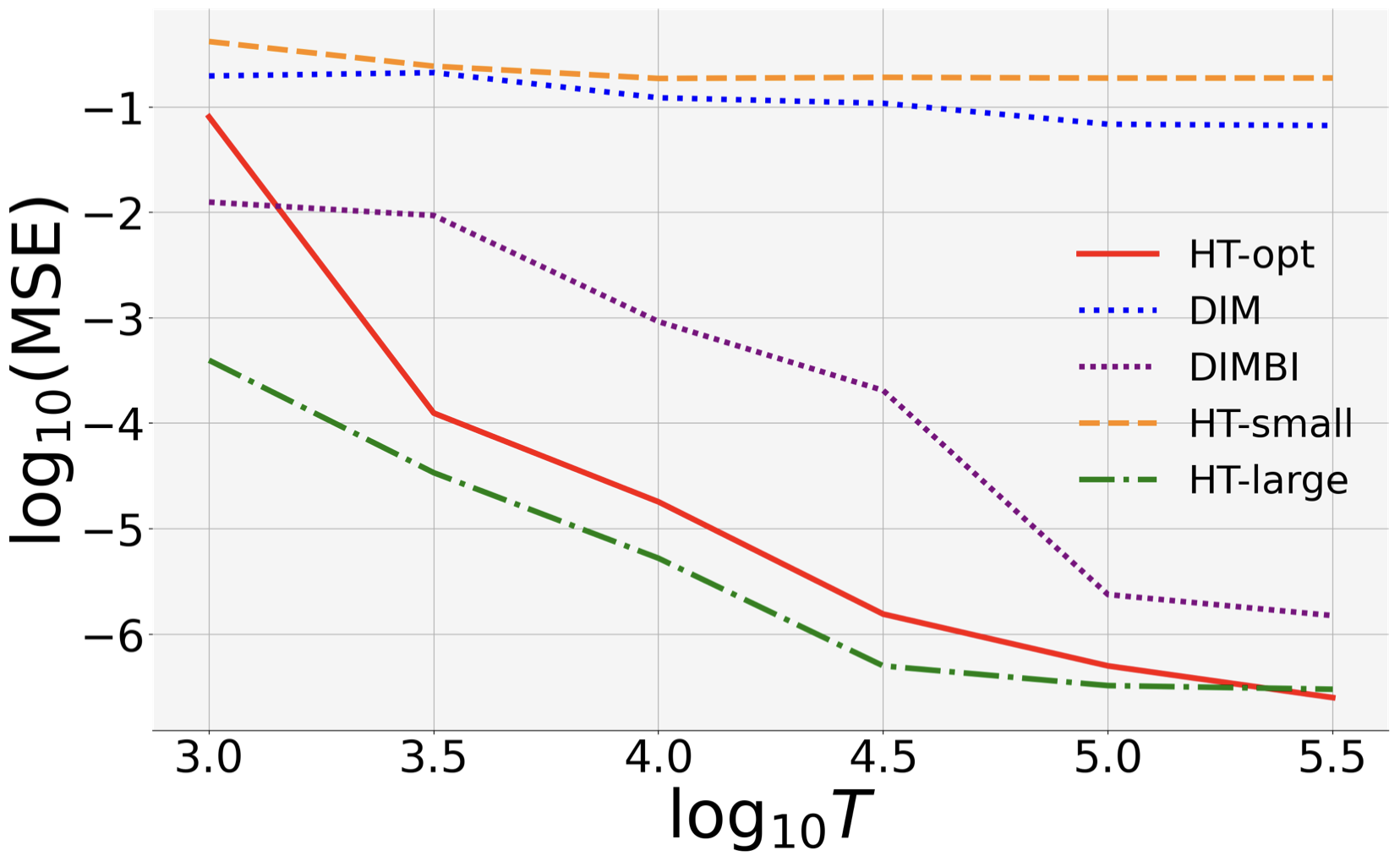
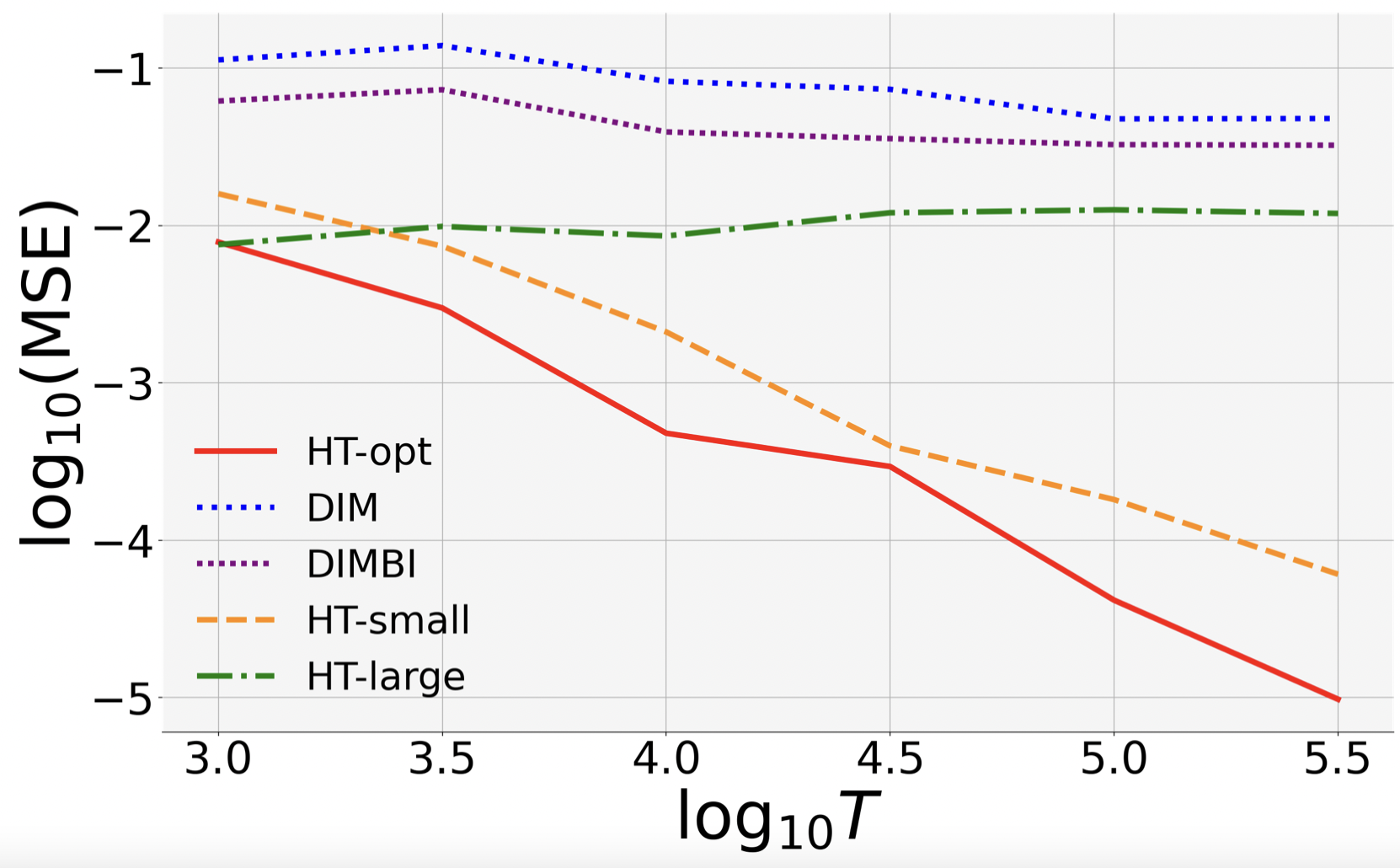
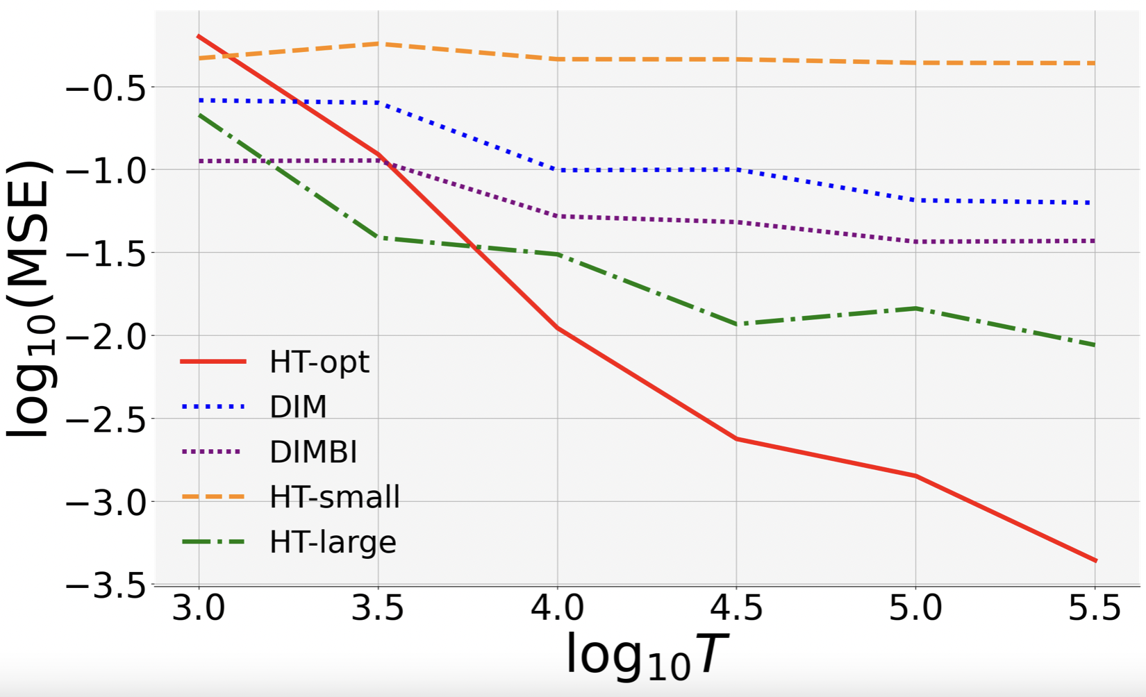
5.1.1 Benchmarks
We compare the MSE and bias of the following five design-estimator combinations.
Note that our MDP has , so we choose .
We will compare:
(1) HT-OPT: HT estimator with block length and radius ;
(2) DIM: difference-in-means estimator (i.e., DIMBI with burn-in ) and block length ,
(3) DIMBI: burn-in , block length ,
(4) HT-small: HT estimator under block length , and radius .
Here we do not choose since its exposure probability is too small and the estimator rarely produces meaningful results.
(5) HT-large: HT estimator with radius under large block length .
Randomly Generated Instances.
For , we randomly generate pairs of sequences as follows.
We consider both stationary and non-stationary setting:
(a) Stationary (Fig. 8 (a), (c)): Set and where i.i.d.
(b) Non-stationary: We introduce both large-scale and small-scale non-stationary.
We first generate a piecewise constant function (called the drift): Partition uniformly into pieces and generate the function values on each piece independently from .
Then, to generate local non-stationarity, we partition uniformly into pieces of lengths , and set if lies in the final fraction of this piece.
5.1.2 Results and Insights
For each instance and block length (), we draw treatment vectors. We visualize the MSE and bias.
The confidence intervals for bias are 95%.
We observe the following.
(a) MSE Rates. HT-opt has the lowest MSE in both statationary and non-stationary settings.
Moreover, its MSE curve in the log-log plots has a slope close to , which validates the theoretical MSE bound.
In contrast, HT-large and DIMBI both perform well in the stationary setting (with a slope close to ), but fail in the non-stationary setting.
(b) DIM(BI) Has Large Bias. DIMBI suffers large bias for both small and large .
This is because for small , DIMBI uses data before the chain mixes sufficiently (even in stationary environment), and therefore suffers large bias.
Large has decent performance when the environment is stationary, but suffers high bias in the presence of non-stationarity. This is because it discards data blindly, and may miss out useful signals in the beginning of a block.
(c) Large leads to high variance.
With large block length, the Markov chain can mix sufficiently and provide reliable data points.
However, the estimator may mistakenly view external non-stationarity as treatment effect.
For example, consider and , then ATE is .
If we have only two blocks, each assigned a distinct treatment (which occurs w.p. ).
Then, the estimated ATE is non-zero.
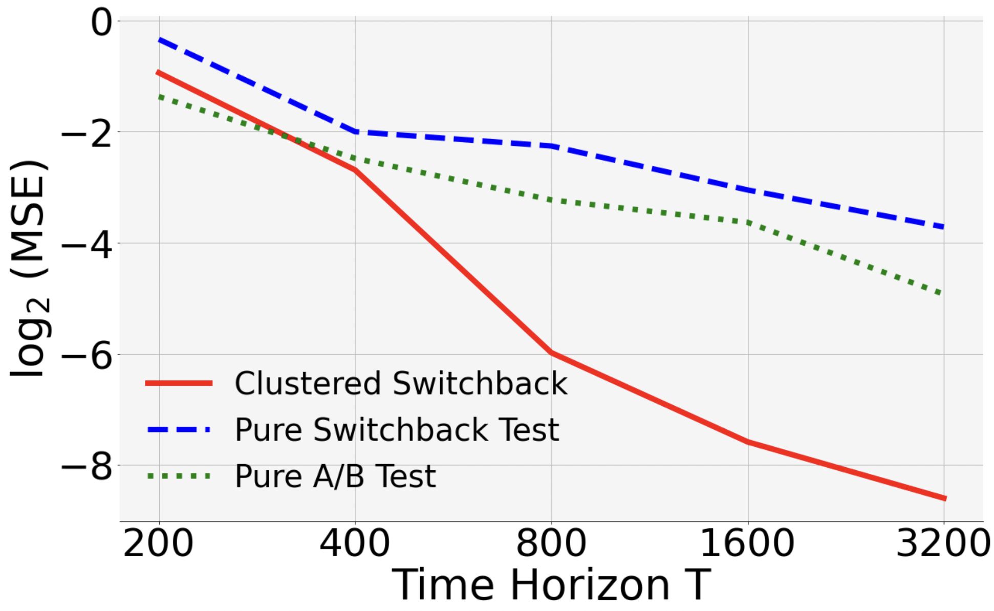
5.2 Multi-unit Setting (General )
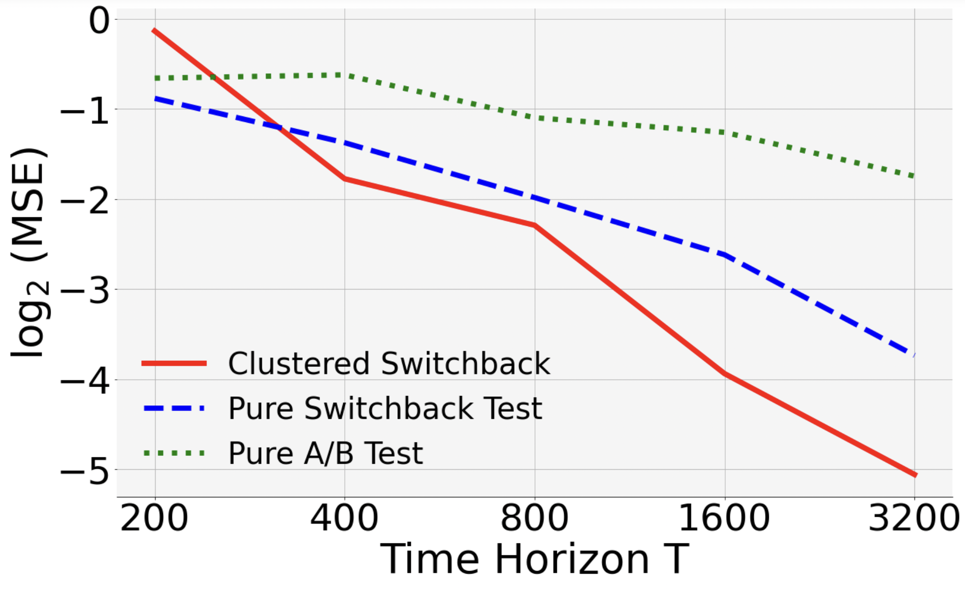
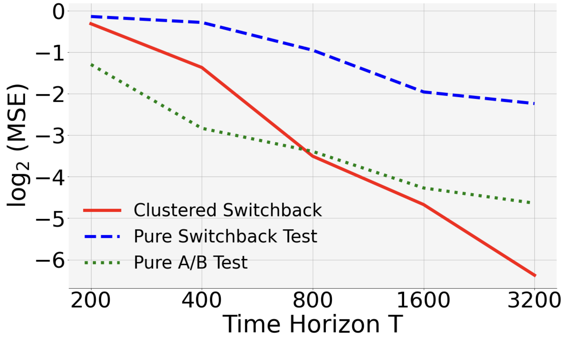
Next, we show that in the presence of both spatial and temporal interference, clustered switchback outperforms both “pure” switchback (i.e., only partition time) and “pure” A/B test (i.e., only partition space).
MDP. Suppose that units lie on an unweighted line graph. Each unit’s state follows the random walk capped at , similar to the single-user setting. To generate spatial interference, we assume that the move-up probability of at time is
In particular, if all -hop neighbors are assigned treatment (resp. 1), then (resp. ). In this setting, the exposure mapping for treatment is equal to if and only if all -hop neighbors are assigned in the previous rounds. As suggested by Corollary 5, we choose .
Reward Function. As in the single-user setting, we choose , where captures large-scale heterogeneity and models user features. To generate ’s, we partition uniformly into pieces of size . We generate the function value on each piece independently from . We also set where i.i.d.
Benchmarks. We partition the space-time into “boxes” of (spatial) width and (temporal) length . We will compare the performance of the HT estimator under the following designs.
(1) Pure Switchback Test: (rate optimal block length for switchback).
(2) Pure A/B Test: (rate optimal width for pure A/B test, see Corollary 5), .
(3) Clustered Switchback Test: (rate optimal width and length).
Discussion. For each , we randomly generated instances and treatment vectors. When , the MSE of clustered switchback decreases most rapidly. The slope of its curve in the log-log is , close to the theoretical value . It also outperforms the other two designs in the other two scenarios.
Finally, let us compare pure A/B with pure switchback. Theoretically, they have MSE rates of and . Consistent with this, our empirical study shows that the MSE of pure A/B test decreases slower than pure switchback when , and faster when .
We repeat the five-curve comparison for different choices of . Recall that in the main body we choose . We now choose and , respectively. As a key observation, we found that the performance of HT-small is heavily based on : It works well for small and not for large ones. This is because the mixing time is almost linear in , so for large , we need more time for the chain to mix sufficiently. But this is difficult for a small block length. In fact, the exposure probability is . So, when and , we have . This means that the exposure mapping discards most of the data points, leading to a high variance.
References
- Aronow et al. [2017] P. M. Aronow, C. Samii, et al. Estimating average causal effects under general interference, with application to a social network experiment. The Annals of Applied Statistics, 11(4):1912–1947, 2017.
- Basse and Airoldi [2018] G. W. Basse and E. M. Airoldi. Model-assisted design of experiments in the presence of network-correlated outcomes. Biometrika, 105(4):849–858, 2018.
- Basse et al. [2019] G. W. Basse, A. Feller, and P. Toulis. Randomization tests of causal effects under interference. Biometrika, 106(2):487–494, 2019.
- Blake and Coey [2014] T. Blake and D. Coey. Why marketplace experimentation is harder than it seems: The role of test-control interference. In Proceedings of the fifteenth ACM conference on Economics and computation, pages 567–582, 2014.
- Bojinov et al. [2023] I. Bojinov, D. Simchi-Levi, and J. Zhao. Design and analysis of switchback experiments. Management Science, 69(7):3759–3777, 2023.
- Cai et al. [2015] J. Cai, A. De Janvry, and E. Sadoulet. Social networks and the decision to insure. American Economic Journal: Applied Economics, 7(2):81–108, 2015.
- Chin [2019] A. Chin. Regression adjustments for estimating the global treatment effect in experiments with interference. Journal of Causal Inference, 7(2), 2019.
- Eckles et al. [2017a] D. Eckles, B. Karrer, and J. Ugander. Design and analysis of experiments in networks: Reducing bias from interference. Journal of Causal Inference, 5(1), 2017a.
- Eckles et al. [2017b] D. Eckles, B. Karrer, and J. Ugander. Design and analysis of experiments in networks: Reducing bias from interference. Journal of Causal Inference, 5(1):20150021, 2017b.
- Farias et al. [2022] V. Farias, A. Li, T. Peng, and A. Zheng. Markovian interference in experiments. Advances in Neural Information Processing Systems, 35:535–549, 2022.
- Forastiere et al. [2021] L. Forastiere, E. M. Airoldi, and F. Mealli. Identification and estimation of treatment and interference effects in observational studies on networks. Journal of the American Statistical Association, 116(534):901–918, 2021.
- Glynn et al. [2020] P. W. Glynn, R. Johari, and M. Rasouli. Adaptive experimental design with temporal interference: A maximum likelihood approach. Advances in Neural Information Processing Systems, 33:15054–15064, 2020.
- Gui et al. [2015] H. Gui, Y. Xu, A. Bhasin, and J. Han. Network a/b testing: From sampling to estimation. In Proceedings of the 24th International Conference on World Wide Web, pages 399–409. International World Wide Web Conferences Steering Committee, 2015.
- Horvitz and Thompson [1952] D. G. Horvitz and D. J. Thompson. A generalization of sampling without replacement from a finite universe. Journal of the American statistical Association, 47(260):663–685, 1952.
- Hu and Wager [2022] Y. Hu and S. Wager. Switchback experiments under geometric mixing. arXiv preprint arXiv:2209.00197, 2022.
- Jagadeesan et al. [2020] R. Jagadeesan, N. S. Pillai, and A. Volfovsky. Designs for estimating the treatment effect in networks with interference. 2020.
- Jiang and Li [2016] N. Jiang and L. Li. Doubly robust off-policy value evaluation for reinforcement learning. In International Conference on Machine Learning, pages 652–661. PMLR, 2016.
- Johari et al. [2022] R. Johari, H. Li, I. Liskovich, and G. Y. Weintraub. Experimental design in two-sided platforms: An analysis of bias. Management Science, 68(10):7069–7089, 2022.
- Kohavi and Thomke [2017] R. Kohavi and S. Thomke. The surprising power of online experiments. Harvard business review, 95(5):74–82, 2017.
- Larsen et al. [2023] N. Larsen, J. Stallrich, S. Sengupta, A. Deng, R. Kohavi, and N. T. Stevens. Statistical challenges in online controlled experiments: A review of a/b testing methodology. The American Statistician, pages 1–15, 2023.
- Leung [2022] M. P. Leung. Rate-optimal cluster-randomized designs for spatial interference. The Annals of Statistics, 50(5):3064–3087, 2022.
- Leung [2023] M. P. Leung. Network cluster-robust inference. Econometrica, 91(2):641–667, 2023.
- Li and Wager [2022] S. Li and S. Wager. Network interference in micro-randomized trials. arXiv preprint arXiv:2202.05356, 2022.
- Li et al. [2023] S. Li, R. Johari, X. Kuang, and S. Wager. Experimenting under stochastic congestion. arXiv preprint arXiv:2302.12093, 2023.
- Li et al. [2021] W. Li, D. L. Sussman, and E. D. Kolaczyk. Causal inference under network interference with noise. arXiv preprint arXiv:2105.04518, 2021.
- Manski [2013] C. F. Manski. Identification of treatment response with social interactions. The Econometrics Journal, 16(1):S1–S23, 2013.
- Ni et al. [2023] T. Ni, I. Bojinov, and J. Zhao. Design of panel experiments with spatial and temporal interference. Available at SSRN 4466598, 2023.
- Sävje [2023] F. Sävje. Causal inference with misspecified exposure mappings: separating definitions and assumptions. Biometrika, page asad019, 2023.
- Sävje [2024] F. Sävje. Causal inference with misspecified exposure mappings: separating definitions and assumptions. Biometrika, 111(1):1–15, 2024.
- Shi et al. [2023] C. Shi, X. Wang, S. Luo, H. Zhu, J. Ye, and R. Song. Dynamic causal effects evaluation in a/b testing with a reinforcement learning framework. Journal of the American Statistical Association, 118(543):2059–2071, 2023.
- Sneider and Tang [2019] C. S. Sneider and Y. Tang. Experiment rigor for switchback experiment analysis. 2019. URL https://careersatdoordash.com/blog/experiment-rigor-for-switchback-experiment-analysis/.
- Sussman and Airoldi [2017] D. L. Sussman and E. M. Airoldi. Elements of estimation theory for causal effects in the presence of network interference. arXiv preprint arXiv:1702.03578, 2017.
- Thomas and Brunskill [2016] P. Thomas and E. Brunskill. Data-efficient off-policy policy evaluation for reinforcement learning. In International Conference on Machine Learning, pages 2139–2148. PMLR, 2016.
- Thomke [2020] S. Thomke. Building a culture of experimentation. Harvard Business Review, 98(2):40–47, 2020.
- Toulis and Kao [2013] P. Toulis and E. Kao. Estimation of causal peer influence effects. In International conference on machine learning, pages 1489–1497. PMLR, 2013.
- Ugander and Yin [2023] J. Ugander and H. Yin. Randomized graph cluster randomization. Journal of Causal Inference, 11(1):20220014, 2023.
- Ugander et al. [2013] J. Ugander, B. Karrer, L. Backstrom, and J. Kleinberg. Graph cluster randomization: Network exposure to multiple universes. In Proceedings of the 19th ACM SIGKDD international conference on Knowledge discovery and data mining, pages 329–337, 2013.
- Wang [2021] Y. Wang. Causal inference with panel data under temporal and spatial interference. arXiv preprint arXiv:2106.15074, 2021.
Appendix A Omitted Proofs in Section 3
A.1 Proof of Theorem 3: MSE Lower Bound
Consider the following two instances . Suppose the interference graph has no edges (and hence there is no interference between isers). We also assume there is only one state and suppress in the notation. The outcomes follow Bernoulli distributions. In , we have for any and treatment . In , for any , the reward functions are given by
The ATE in these two instances are and respectively.
Now fix any design (i.e., random vector taking value in ). Let be the probability measures induced by the two instances, and be the marginal probability measures. Note that the outcomes distributions are Bernoulli, so for each . Therefore,
| (2) |
In particular, for , we have .
To conclude, consider any estimator and the event that . By Pinsker’s inequality,
Therefore, we have either or . Therefore, we have
| ∎ |
A.2 Proof of Corollary 1
Observe that for the singleton partition, if and only if . Moreover, since , the interval intersects at most two time blocks, so for any . This,
Therefore, by Theorem 1,
| ∎ |
A.3 Proof of Corollary 2
Since , the interval intersects at most two time blocks. This, for any . Therefore,
| ∎ |
A.4 Proof of Corollary 3
Note that for , the dependence graph is the second power111i.e., add an edge between two nodes if their hop distance is at most . of the interference graph. Since every node has a maximum degree , each node has degree no more than edges in the dependence graph. Moreover, since , the interval intersects at most two time blocks, and so each depends on at most cluster-blocks, so for any . Therefore,
| ∎ |
A.5 Proof of Corollary 5
To find , consider a unit with . Then, there exists such that and and hence lies in either or one of the eight clisters neighboring . Therefore,
| ∎ |
A.6 Proof of Proposition 4
Suppose intersects clusters (i.e., spatio-blocks) , and . Then,
Denote by the treatment assigned to . Recall that the -FNE requires that
| (3) |
for either or . Suppose ; the proof for is identical by symmetry. Then, Eq. 3 can be rewritten as
Since ’s are i.i.d. Bernoulli, we have
Since the interval intersects time blocks, the claim follows by taking
| ∎ |
Appendix B Bias Analysis: Proof of Proposition 2
For any event -measurable event , denote by , , , and probability, expectation, variance, and covariance conditioned on .
Next, we show that 1 implies a bound on how the law of under can vary as we vary . In particular, when is a singleton set, we use the subscript instead of .
Lemma 2 (Decaying Temporal Interference).
Consider any with and . Suppose are identical on . Then,
Proof.
For any , we denote and . Then, for any , by the Chapman–Kolmogorov equation,
This, if ,
where we ised in the second equality and 1 in the inequality. Applying the above for all , we conclude that
where the first inequality is becaise , and the last is becaise the TV distance is at most . ∎
Based on Lemma 2, we can establish the following bound.
Lemma 3 (Per-unit Bias).
For any , , and , we have
Proof.
For any , and , we have
Note that implies that on . Therefore, by Lemma 2 with , we obtain
and hence
| ∎ |
Now we are prepared to prove Proposition 2. Recall that and .
Proof of Proposition 2.
By Lemma 3,
| ∎ |
Appendix C Variance Analysis: Proof of Proposition 3
We start with a bound that holds for all pairs of units. Note that for any , since treatment and control are assigned with equal probabilities. We will this suppress in the notation.
Lemma 4 (Covariance Bound).
For any , and , we have
Proof.
Expanding the definition of , we have
| (4) |
where the last inequality is by the Cauchy-Schwarz inequality. Note that is binary and
we have
| ∎ |
The above bound alone is not sufficient for our analysis, as it does not take advantage of the rapid mixing property. In the rest of this section, we show that for any units that are far apart in time, the covariance of their HT terms decays exponentially in their temporal distance.
C.1 Covariance of Outcomes
We first show that if the realization of one random variable has little impact on the (conditional) distribution of another random variable, then they have low covariance.
Lemma 5 (Low Interference in Conditional Distribution Implies Low Covariance).
Let be two random variables and be real-valued functions defined on their respective realization spaces. If for some , we have
then,
Proof.
Denote by the probability measures of , , , and conditioned on , respectively. We then have
| ∎ |
Viewing as outcomes in different rounds, we ise the above to bound the covariance in the outcomes in terms of their temporal distance.
Lemma 6 (Covariance of Outcomes).
For any , and , we have
Proof.
Wlog assume . Recall that , so
The latter three terms are zero by the exogenois noise assumption (in terms of covariances). By Lemma 2 and the triangle inequality for , for any , we have
| (5) |
where denotes the Dirac distribution at , and the last inequality follows since the TV distance between any two distributions is at most .
Now, apply Lemma 5 with in the role of , with in the role of , with in the role of , with in the role of , and with in the role of . Noting that and combining with Section C.1, we conclude the statement. ∎
C.2 Covariance of HT terms
So far we have shown that the outcomes have low covariance if they are far apart in time. However, this does not immediately imply that the covariance between the HT terms is also low, since each HT term is a product of the outcome and the exposure mapping. To proceed, we need the following.
Lemma 7 (Bounding Covariance Using Conditional Covariance).
Let be independent Bernoulli random variables with means . Suppose are random variables s.t.
Then,
Proof.
Since are Bernoulli, we have
| (6) |
Note that and , so
and therefore
| ∎ |
We obtain the following bound by applying the above to the outcomes and exposure mappings in two rounds that are in different blocks and are further apart than (in time).
Lemma 8 (Covariance of Far-apart HT terms).
Suppose and satisfy and , then
Proof.
Observe that for any (possibly identical) , since lie in distinct blocks and are more than apart, we see that and are independent. This, by Lemma 7, we have
| (7) |
To bound the above, consider the event
so that by Lemma 6,
The conclision follows by summing over all four combinations of . ∎
Remark 5.
The restriction that are both farther than apart in time and lie in distinct blocks are both necessary for the above exponential covariance bound. As an example, fix a vertex and consider in the same block and suppose that they are at a distance away from the boundary of this block. Then, the exposure mappings and are the same, which we denote by . Then,
where . Therefore, we can choose the mean outcome function to be large so that the above does not decrease exponentially in .
C.3 Proof of Proposition 3
We are now ready to bound the variance. Write
| (8) |
We need two observations to decompose the above. First, by the definition of the dependence graph, if , then . This, for each , we may consider only the units with . Second, observe that if , then we can apply Lemma 8 to bound the covariance term exponentially in . Combining, we can decompose Eq. 8 into close-by (“C”) and far-apart (“F”) pairs as
| (9) |
where
and
To further analyze the above, fix any .
Part II: Bounding . By Lemma 8,
| (11) |
where the “2” in the inequality arises since may be either greater or smaller than .
Combining Sections C.3 and C.3, we conclude that
| ∎ |