icml

ClassContrast: Bridging the Spatial and Contextual Gaps for Node Representations

Md Joshem Uddin¹, Astrit Tola¹, Varin Sikand¹, Cuneyt Gurcan Akcora², Baris Coskunuzer¹

Abstract

Graph Neural Networks (GNNs) have revolutionized the domain of graph representation learning by utilizing neighborhood aggregation schemes in many popular architectures, such as message passing graph neural networks (MPGNNs). This scheme involves iteratively calculating a node’s representation vector by aggregating and transforming the representation vectors of its adjacent nodes. Despite their effectiveness, MPGNNs face significant issues, such as oversquashing, oversmoothing, and underreaching, which hamper their effectiveness. Additionally, the reliance of MPGNNs on the homophily assumption, where edges typically connect nodes with similar labels and features, limits their performance in heterophilic contexts, where connected nodes often have significant differences. This necessitates the development of models that can operate effectively in both homophilic and heterophilic settings.

In this paper, we propose a novel approach, ClassContrast, grounded in Energy Landscape Theory from Chemical Physics, to overcome these limitations. ClassContrast combines spatial and contextual information, leveraging a physics-inspired energy landscape to model node embeddings that are both discriminative and robust across homophilic and heterophilic settings. Our approach introduces contrast-based homophily matrices to enhance the understanding of class interactions and tendencies. Through extensive experiments, we demonstrate that ClassContrast outperforms traditional GNNs in node classification and link prediction tasks, proving its effectiveness and versatility in diverse real-world scenarios.

Code — https://anonymous.4open.science/r/CC-77A6/

1 Introduction

Over the past decade, GNNs have made a breakthrough in graph machine learning by adapting several deep learning models, originally developed for domains such as computer vision and natural language processing, to the graph setting (Section 2) . By using different approaches and architectures, GNNs produce powerful node embeddings by integrating neighborhood information with domain features. While recent GNN models consistently outperform the state-of-the-art (SOTA) results, in the seminal papers (Xu et al. 2019; Morris et al. 2019), the authors showed that the expressive power of message passing GNNs (MP-GNNs) is about the same as a well-known former method in graph representation learning, i.e. the Weisfeiler-Lehman algorithm (Shervashidze et al. 2011). Furthermore, recent studies show that GNNs suffer from significant challenges like oversquashing (Topping et al. 2021), oversmoothing (Oono and Suzuki 2020), and underreaching (Barceló et al. 2020).

Another major issue with MPGNNs is their reliance on the (useful) homophily assumption, where edges typically connect nodes sharing similar labels and node features networks (Sen et al. 2008). However, many real-world scenarios exhibit heterophilic behavior, such as in protein and web networks (Pei et al. 2019) where conventional GNNs (Hamilton et al. 2017; Veličković et al. 2018a) may experience significant performance degradation, sometimes even underperforming compared to a multilayer perceptron (MLP) (Zhu et al. 2020; Luan et al. 2022). Therefore, there is a pressing need to develop models that function effectively in both homophilic and heterophilic settings.

We hypothesize that the limitations in current methods arise from the ineffective utilization of two key types of information in graphs: spatial information, which captures the local neighborhood’s class distribution for each node, and contextual information, which assesses each node’s similarity or dissimilarity to class representatives within a latent space, incorporating information from relevant but distant nodes. To address this issue, we leverage Energy Landscape Theory (Wales 2002; Wales et al. 1998) from Chemical Physics, a framework used to describe and analyze the behavior of complex systems, such as protein folding (Plotkin and Onuchic 2002). This theory visualizes the potential energy of a system as a multidimensional landscape, with valleys and peaks representing states of different energies.

We apply this theory to model a node’s position within a network, aiming to understand how nodes form connections based on specific contextual influences encoded as node attributes. In ClassContrast, integrating spatial and contextual information is similar to navigating an energy landscape where each node’s embedding seeks a low-energy state that is both highly discriminative and informative. In a homophilic setting, this state ideally balances similarity to nodes within the same class (lowering energy) and dissimilarity to nodes in different classes (avoiding overly general local minima). In a heterophilic setting, the model uses both types of information to address the complexities of non-conforming node relationships, where nodes that are dissimilar may still be connected. The energy landscape model helps identify and strengthen valuable connections that cross traditional boundaries, enhancing the model’s classification accuracy in environments with non-standard “like-likes-like” patterns. This dual capability allows ClassContrast to generate robust embeddings that perform well across varied graph structures, regardless of network homophily or heterophily.

Overall, ClassContrast effectively integrates spatial and contextual information to produce robust node embeddings, demonstrating impressive performance in node classification and link prediction tasks.

Our contributions can be summarized as follows:

$\bullet$

We propose a physics-inspired approach, leveraging Energy Landscape Theory, to construct class-aware node representations.
$\bullet$

We introduce contrast-based homophily matrices that provide detailed insights into interactions and homophily tendencies among classes.
$\bullet$

Our ClassContrast framework combines spatial and contextual information, achieving highly competitive results with state-of-the-art GNNs in both node classification and link prediction tasks.
$\bullet$

Our experiments show that ClassContrast can be smoothly integrated with GNN models, boosting performance across both homophilic and heterophilic settings, proving its versatility across various real-world applications.

2 Related Work

Over the past decade, GNNs have dominated graph representation learning, especially excelling in node classification tasks (Xiao et al. 2022). After the success of Graph Convolutional Networks (GCN) (Kipf and Welling 2017), using a neighborhood aggregation strategy to perform convolution operations on graph, subsequent efforts focused on modifying, approximating, and extending the GCN approach, e.g., involving attention mechanisms (GAT) (Veličković et al. 2018a), sampling and aggregating information from a node’s local neighborhood (GraphSAGE) (Hamilton et al. 2017). However, a notable scalability challenge arose due to its dependence on knowing the full graph Laplacian during training. To address this limitation, numerous works emerged to enhance node classification based on GCN, such as methods , importance sampling node (FastGCN) (Chen, Ma, and Xiao 2018), adaptive layer-wise sampling with skip connections (ASGCN) (Huang et al. 2018), adapting deep layers to GCN architectures (deepGCN) (Li et al. 2019), incorporating node-feature convolutional layers (NFC-GCN) (Zhang et al. 2022).

Two fundamental shortcomings of MPGNNs are the loss of structural information within node neighborhoods and the difficulty in capturing long-range dependencies. To address these inherent issues, numerous studies conducted in the past few years have introduced various enhancements. These improvements encompass diverse aggregation schemes, such as skip connections(Chen et al. 2020), geometric methods(Pei et al. 2019), aiming to mitigate the risk of losing crucial information. Additionally, advancements like implicit hidden layers (Geng et al. 2021) and multiscale modeling (Liu et al. 2022) have been explored to augment the GNN’s capabilities.

Another major issue with MPGNNs is that they operate under the homophily assumption and exhibit poor performance in heterophilic networks (Zhu et al. 2020; Luan et al. 2023). Hence, in the past few years, various efforts have been undertaken to develop GNNs that function effectively in heterophilic settings (Pei et al. 2019; Lim et al. 2021a; Luan et al. 2022; Zheng et al. 2022; Xu et al. 2023).

However, to the best of our knowledge, no previous work has developed a systematic approach to analyze class-wise relations.

3 Energy Landscape Theory and Its Application to Node Representation

Energy Landscape Theory originates from the field of chemical physics (Wales 2002), where it is utilized to describe the potential energy of a molecular system as a multidimensional landscape. This landscape is characterized by a series of valleys and peaks, each representing different states of energy. Valleys correspond to stable states (or low-energy configurations) where a system tends to reside under normal conditions, while peaks represent high-energy states that are less likely to be occupied.

In the context of graph neural networks, we apply the principles of Energy Landscape Theory to the problem of node representation learning. Here, we envisage nodes as entities navigating through an ’energy landscape’ constructed from the network structure and node attributes (see Appendix E for connections to the Structural Balance Theory (Heider 1946) on social networks). This landscape is shaped by the distribution of node features and the topological arrangement of the graph, wherein each node seeks a position corresponding to a state of minimal energy. For example, a fundamental result in social networks states that nodes aim to close friendship triangles (Granovetter 1973) to achieve a lower state (and foster trust). The absence of closed triangles indicates higher energy states, which may signify weaker relationships or even potential animosity. Such relationships are studied in signed network analysis using balance and structural theories (Leskovec, Huttenlocher, and Kleinberg 2010). We analogously define energy states by the optimal embedding that reflects accurate class membership and distinctiveness from nodes of different classes, which we measure with a class-aware definition of homophily (see Section 4.4). This approach allows us to conceptualize the embedding process as a dynamic system where nodes move towards lower-energy configurations that represent stable, informative, and discriminative embeddings in the context of the given graph.

Why is Energy Landscape Approach Useful?

We posit that a graph exhibits not merely a singular energy peak or valley, but multiple such features shaped by group formation dynamics. Consequently, nodes may display either homophilous or heterophilous behaviors depending on their group affiliations within a single graph. This variability implies that node representation should not uniformly assume proximity of neighbors as a reliable descriptor of a node’s characteristics. For example, Zhu et al. report that “in the Chameleon dataset, intra-class similarity is generally higher than inter-class similarity so MLP works better than GCN” (Zhu et al. 2020). Therefore, message-passing-based schemes should be employed selectively, based primarily on the presence of demonstrable homophily within groups. In the absence of such homophily, the system should learn to model heterophilic behaviors effectively. To this end, we claim that our framework, ClassContrast, is capable of simultaneously modeling both homophilous and heterophilous behaviors, adapting its approach as necessary for different groups.

We begin by detailing ClassContrast, focusing on two primary objectives: the discovery of spatial and contextual information. The first objective is to extract information from the node’s neighborhood (spatial), while the second is to derive insights from the node’s domain attributes (contextual). Our framework is visualized in Figure 1.

4 ClassContrast Embeddings

Refer to caption — Figure 1: ClassContrast framework. Spatial and contextual embeddings are incorporated in class-aware contrast-based learning.

In the following discussion, we adhere to the notation $\mathcal{G}=(\mathcal{V},\mathcal{E},\mathcal{W},\mathcal{X})$ where $\mathcal{V}=\{v_{i}\}_{i=1}^{m}$ represents the vertices (nodes), $\mathcal{E}=\{e_{ij}\}$ represents edges, $\mathcal{W}=\{\omega_{ij}\subset\mathbb{R}^{+}\}$ represents edge weights, and $\mathcal{X}=\{X_{i}\}_{i=1}^{m}\subset\mathbb{R}^{n}$ represents node features. If no node features are provided, $\mathcal{X}=\emptyset$ . Consider a graph where nodes are categorized into $N$ classes. For each node $u$ , we aim to construct an embedding $\vec{\gamma}(u)$ of dimension $q\times N$ , where $q$ is determined by specifics of the graph such as its directedness, weighted nature, and the format of domain features.

Specifically, we generate spatial embeddings $\{\vec{\alpha}_{1}(u),\vec{\alpha}_{2}(u),\dots\}$ , derived from local neighborhood information, and contextual embeddings $\{\vec{\beta}_{1}(u),\vec{\beta}_{2}(u),\dots\}$ , derived from node properties specific to the domain. Each embedding, $\vec{\alpha}_{i}(u)$ and $\vec{\beta}_{j}(u)$ , is $N$ -dimensional, with one entry corresponding to each class (ClassContrast coordinates). These embeddings are then concatenated to form the final embedding $\vec{\gamma}(u)$ of size $q\times N$ . For simplicity, we focus on applications in an inductive setting. In Section C.2, we discuss adaptations of our methods to accommodate transductive settings.

4.1 Spatial Node Embedding

Spatial node embedding leverages the structure of a graph to measure the proximity of a node to various known classes within that graph. For each node $u$ in the graph $\mathcal{G}$ with vertices $\mathcal{V}$ , the $k$ -hop neighborhood of $u$ , denoted as $\mathcal{N}_{k}(u)$ , includes all vertices $v$ such that the shortest path distance $d(u,v)$ between $u$ and $v$ is at most $k$ hops: $\mathcal{N}_{k}(u)=\{v\in\mathcal{V}\mid d(u,v)\leq k\}$ . Here, $d(u,v)$ represents the shortest path length between $u$ and $v$ . If no path exists, then $d(u,v)=\infty$ . In the case of a directed graph $\mathcal{G}$ , edge directions are disregarded when calculating distances.

Assume that there are $N$ classes of nodes, represented as $\mathcal{C}_{1},\mathcal{C}_{2},\dots,\mathcal{C}_{N}$ . Let $\mathcal{V}_{\text{train}}$ be the set of nodes with known labels in the training dataset.

The feature vector $\vec{\alpha}_{k}(u)$ for node $u$ is initialized as the distribution of class occurrences: $\vec{\alpha}_{k}(u)=[a_{k1},a_{k2},\dots,a_{kN}]$ where $a_{kj}$ counts how many neighbors of $u$ belong to class $\mathcal{C}_{j}$ within the k-hop neighborhood intersecting with $\mathcal{V}_{\text{train}}$ : $a_{kj}=|\{v\in\mathcal{C}_{j}\mid v\in\mathcal{N}_{k}(u)\cap\mathcal{V}_{\text{train}}\}|$ . Consider the toy example of Figure 2(a), where the (k=1)-hop neighborhood of node $u$ contains node $z$ from class $1$ and node $y$ from class $2$ . As a result, $\vec{\alpha}_{1}(u)=[1\ 1\ 0]$ . We extend the spatial embeddings to directed and weighted graph cases by incorporating edge directions and weights in additional dimensions (see Appendix Section C.3) for the definitions.

4.2 Contextual Node Embedding

Inspired by Energy Landscapes, contextual node embeddings utilize the attribute space to measure the distance of a node to known classes. In social networks, node attributes might include user-specific details (Mislove et al. 2007), while in citation networks, they often involve the presence or absence of certain keywords (Tang et al. 2008). These attributes are crucial for predicting node behavior as they provide intrinsic information about the nodes themselves. Hence, we develop a general and versatile approach to effectively utilize this information in node classification task.

We use the term contextual node embeddings to highlight the importance of context within the graph structure, beyond isolated node attributes. Unlike attribute embeddings, which embed node characteristics directly, contextual node embeddings integrate the node’s attributes and its relational and structural position in the graph. This is crucial in scenarios where class behavior and node features interact, such as an article’s topic influencing its citation links.

A real-life context example.

Consider the CORA dataset where publications that are frequently cited by other papers, especially by those within the same class (topic), may be considered authoritative in their field. An embedding that captures this citation context can differentiate between a highly influential paper and one that is similarly cited (by papers from other classes) but less authoritative.

In contextual embeddings we identify two cases on attribute availability and quality. First, attributes may already be available in high quality vectors, such as word embeddings (e.g., word2vec (Mikolov et al. 2013a, b)). We directly integrate these vectors without additional processing, as detailed in Appendix D. When node attributes are available but unprocessed, we define an attribute vector $\mathcal{X}(u)$ for each node $u$ , which maps nodes to an $n$ -dimensional real vector space. For each class $\mathcal{C}_{j}$ , we identify a cluster of points $\mathcal{Z}_{j}=\{\mathcal{X}(u)\mid u\in\mathcal{C}_{j}\}$ and establish a representative landmark $\xi_{j}$ in $\mathbb{R}^{n}$ for this cluster.

Definition 4.1 (Class Landmark).

Given a node class $\mathcal{C}_{j}$ and its corresponding cluster of node embeddings $\mathcal{Z}_{j}$ , the landmark $\xi_{j}$ is computed as the centroid of the points in $\mathcal{Z}_{j}$ , normalized by the number of nodes in $\mathcal{C}_{j}$ : $\xi_{j}=\frac{1}{|\mathcal{C}_{j}|}\sum_{u\in\mathcal{C}_{j}}\mathcal{X}(u).$

Definition 4.2 (Distances to Class Landmarks).

Let $\mathbf{d}$ be a metric that measures the distance in $\mathbb{R}^{n}$ . For a node $u$ with an embedding $\mathcal{X}(u)$ , the distance to the class landmark $\xi_{j}$ is defined as: $d_{j}=\mathbf{d}(\mathcal{X}(u),\xi_{j})$ for each class $\mathcal{C}_{j}$ . These distances $d_{j}$ help in assessing how similar or distinct the node is from each class represented by the landmarks.

Definition 4.3 (Contextual Embedding).

Given a node $u$ and a set of class landmarks $\{\xi_{j}\}\subseteq\mathbb{R}^{n}$ , one for each class $\mathcal{C}_{j}$ , the contextual embedding of node $u$ is defined by a vector of distances from the node’s embedding to each class landmark: $\vec{\beta}(u)=[d_{1},d_{2},d_{3},\dots,d_{N}]$ where $d_{j}=\mathbf{d}(\mathcal{X}(u),\xi_{j})$ for each class $\mathcal{C}_{j}$ (see Figure 2(b)). This vector $\vec{\beta}(u)$ encapsulates the node’s position relative to each class within the attribute space.

Landmark Sets.

To obtain information about the domain attributes of nodes for each class, multiple landmarks can be defined. For instance, while the first landmark $\xi^{1}_{j}\in\mathbb{R}^{n}$ represents the center of each cluster $\mathcal{Z}_{j}$ , the second landmark $\xi^{2}_{j}\in\mathbb{R}^{n}$ may capture the most frequent attributes of $\mathcal{Z}_{j}$ (see Appendix D). For each type of landmark, a corresponding distance or similarity measure $\mathbf{d}^{k}(.,.)$ is defined, such as Euclidean or cosine distance for real-valued attribute vectors, or Jaccard similarity for categorical attributes (Niwattanakul et al. 2013). Subsequently, another $N$ -dimensional vector $\vec{\beta}_{k}(u)=[d_{k1},d_{k2},d_{k3},\dots,d_{kN}]$ is obtained, where $d_{kj}=\mathbf{d}^{k}(\mathcal{X}(u),\xi^{k}_{j})$ for each class $\mathcal{C}_{j}$ . Landmark set extensions are explained in Appendix D.

4.3 ClassContrast Embedding

We may expand spatial neighborhoods, and extend landmark sets arbitrarily. However, for exposition purposes, we will define ClassContrast embeddings over a directed graph where each node’s neighborhood is considered up to two hops and each class $\mathcal{C}_{j}$ has two landmarks. We define the ClassContrast Embedding of a node $u$ by concatenating spatial and contextual embeddings. Specifically, we consider:

$\bullet$ Spatial embeddings from incoming and outgoing 1-hop neighborhoods ( $\vec{\alpha}_{1i}(u)$ and $\vec{\alpha}_{1o}(u)$ ) and the 2-hop neighborhood ( $\vec{\alpha}_{2}(u)$ ).

$\bullet$ Contextual embeddings based on distances to two class landmarks ( $\vec{\beta}_{1}(u)$ and $\vec{\beta}_{2}(u)$ ), representing domain-specific characteristics.

Definition 4.4 (ClassContrast Embedding).

The final embedding $\vec{\gamma}(u)$ for node $u$ is a concatenated vector of these embeddings, resulting in a $5\cdot N$ -dimensional vector where $N$ is the number of classes. For clarity, we represent $\vec{\gamma}(u)$ in a 2D format ( $m\times N$ ) where each column corresponds to one class, and each row represents one type of "contrast" vector:

$\vec{\gamma}(u)=\left[{\begin{array}[]{lcr}\longleftarrow&\vec{\alpha}_{1i}(u)&\longrightarrow\\ \longleftarrow&\vec{\alpha}_{1o}(u)&\longrightarrow\\ \longleftarrow&\vec{\alpha}_{2}(u)&\longrightarrow\\ \longleftarrow&\vec{\beta}_{1}(u)&\longrightarrow\\ \longleftarrow&\vec{\beta}_{2}(u)&\longrightarrow\end{array}}\right]{\begin{array}[]{ll}\mbox{Spatial}&\mbox{Incoming 1-ngbd}\\ \mbox{Spatial}&\mbox{Outgoing 1-ngbd}\\ \mbox{Spatial}&\mbox{2-ngbd}\\ \mbox{Contextual}&\{d(\mathcal{X}_{u},\xi^{1}_{j})\}\\ \mbox{Contextual}&\{d(\mathcal{X}_{u},\xi^{2}_{j})\}\end{array}}$

4.4 Homophily and ClassContrast

In this section, we develop the final component of the energy landscape theory for ClassContrast that will enable us to quantify the energy landscapes between classes.

In recent years, several metrics have been introduced to study the effect of homophily on graph representation learning (Lim et al. 2021b; Jin et al. 2022; Luan et al. 2022; Platonov et al. 2023) (see overview in Section B.1). A widely used metric, the node homophily ratio, is defined as $\mathcal{H}_{\mbox{node}}(\mathcal{G})=\frac{1}{|\mathcal{V}|}\sum_{v\in\mathcal{V}}\frac{\eta(v)}{deg(v)}$ , where $\eta(v)$ represents the number of adjacent nodes to $v$ sharing the same class. A graph $\mathcal{G}$ is termed homophilic if $\mathcal{H}_{\mbox{node}}(\mathcal{G})\geq 0.5$ , and heterophilic otherwise.

Although homophily measures similarity across an entire graph, individual groups within a graph may display different homophily behaviors. Our ClassContrast approach leverages class interactions and introduces a class-aware homophily score through non-symmetric measures:

Definition 4.5 (ClassContrast (CC) Homophily Matrices).

Let $(\mathcal{G},\mathcal{V})$ be graph with node classes $\{\mathcal{C}_{1},\mathcal{C}_{2},\dots,\mathcal{C}_{N}\}$ . Let $\vec{\alpha}$ be a spatial or contextual embedding. We define the homophily rate between classes $i$ and $j$ as $h^{\alpha}_{ij}=\frac{1}{|\mathcal{C}_{i}|}\sum_{v\in\mathcal{C}_{i}}\frac{\alpha_{v}^{j}}{|\alpha_{v}|}$ where $\alpha_{v}^{j}$ is the $j^{th}$ entry of $\vec{\alpha}_{v}$ . Considering pairwise homophily rates of all classes, we create the $N\times N$ matrix $\mathcal{\textbf{M}}=[h^{\alpha}_{ij}]$ as the $\alpha$ Homophily Matrix of $\mathcal{G}$ .

In Appendix Table 9, we provide examples of CC homophily matrices. This matrix $\mathbf{M}$ provides detailed insights into both intra-class (homophily) and inter-class (heterophily) interactions, with diagonal elements indicating the propensity for nodes to connect within their own class.

Definition 4.6 ( $\alpha$ Homophily Ratio).

For a given $\alpha$ Homophily Matrix $\mathcal{M}^{\alpha}$ , $\alpha$ Homophily $\mathcal{H}^{\alpha}_{cc}$ is defined as the average of the diagonal elements. i.e, $\mathcal{H}^{\alpha}_{cc}=\frac{1}{N}\sum_{i=1}^{N}h_{ii}$ .

For example, the Spatial-1 Homophily ratio reveals a node’s likelihood to connect with nodes of the same class within its immediate neighborhood. Homophily matrices not only introduce new ways to measure homophily but also relates to various existing homophily metrics:

Theorem 4.7.

For a given $\mathcal{G}=(\mathcal{V},\mathcal{E})$ , let $\vec{\alpha}_{1}(v)$ be CC spatial-1 vector. Let $\widehat{\alpha}_{1}(v)$ be the vector where the entry corresponding to the class of $v$ is set to $0$ . Then, $1-\mathcal{H}_{\mbox{node}}(\mathcal{G})=\frac{1}{|\mathcal{V}|}\sum_{v\in\mathcal{V}}\frac{\|\widehat{\alpha}_{1}(v)\|_{1}}{\|\vec{\alpha}_{1}(v)\|_{1}}$ .

The proof of this theorem and further discussions on how our ClassContrast homophily relates to other forms of homophily are detailed in the Appendix B.

5 Experiments

We evaluate ClassContrast in two tasks: node classification and link prediction. We share our Python implementation at https://anonymous.4open.science/r/CC-77A6/

Datasets.

We use three widely-used homophilic datasets which are citation networks, CORA, CITESEER, and PUBMED (Sen et al. 2008), two Open Graph Benchmark (OGB) datasets: OGBN-ARXIV and OGBN-MAG (Hu et al. 2020), and five heterophilic datasets, TEXAS, CORNELL, WISCONSIN, CHAMELEON and SQUIRREL (Pei et al. 2019). The datasets are described in Appendix D and their statistics are given in Table 1.

Model Setup and Metrics.

For the three citation networks and five heterophilic datasets, the same setup is used as outlined by Bodnar et al. (Bodnar et al. 2022): we split nodes of each class into 48%, 32%, and 20% for training, validation and testing and report averages of 10 runs. We follow the train/validation/test split set by the OGB to report the accuracy score for OGBN-ARXIV and OGBN-MAG (Hu et al. 2020).

Embeddings.

We give the details of ClassContrast embeddings for each dataset in appendix D. The dimensions of the embeddings used for each dataset are given in Table 11.

Model Hyperparameters.

ClassContrast uses an MLP classifier (Haykin 1998). We configure the architecture with $700$ neurons for the hidden layers, a learning rate of $0.001$ , and employed the Adam optimization method for training for 500 epochs. We utilized the ReLU activation function for the hidden layers and applied a L2 regularization value of $0.00001$ to mitigate overfitting.

Hardware.

We ran non-OGB experiments on a machine with Apple m2 chip Processor (8-core CPU, 10-core GPU, and, 6-core Neural Engine), and 16Gb of RAM. For the OGB data sets, we ran experiments on Google Colab with Intel(R) processor, 2.20GHz CPU, V100 GPUs, and 25.5Gb of RAM.

Runtime.

ClassContrast is computationally efficient. ClassContrast requires approximately $4$ hours for OGBN-ARXIV and $10$ hours for OGB-MAG to create all embeddings, and about $10$ minutes to train for all OGB datasets. End-to-end, our model processes three citation network datasets and three WebKb datasets, including the CHAMELEON dataset, in under a minute. Moreover, PUBMED takes about $20$ minutes and SQUIRREL approximately $3$ minutes. For comparison, RevGNN-Deep requires $13.5$ days and RevGNN-Wide takes $17.1$ days to train for 2000 epochs on a single NVIDIA V100 for the OGB datasets.

5.1 Node Classification Results

Baselines.

We compare ClassContrast with 12 state-of-the-art models (Table 2) and three classical models: GCN (Kipf and Welling 2017), GraphSage (Hamilton et al. 2017) and GAT (Veličković et al. 2018a). We choose ALT-APPNP (Liang et al. 2023) and LRGNN (Liang et al. 2023) SOTA models as they are recent and outperform the competitors in their respective papers. All baselines in Tables 2 and 3 use the transductive setting except for GraphSAGE, which uses the inductive setting.

Table 1: Benchmark datasets for node classification.

Datasets	Nodes	Edges	Classes	Features	Tr/Val/Test ( $\%$ )	Hom.
CORA	2,708	5,429	7	1,433	48/32/20	0.83
CITESEER	3,312	4,732	6	3,703	48/32/20	0.72
PUBMED	19,717	44,338	3	500	48/32/20	0.79
OGBN-ARXIV	169,343	1,166,243	40	128	OGB	0.65
OGBN-MAG	1,939,743	21,111,007	349	128	OGB	0.30
TEXAS	183	309	5	1,703	48/32/20	0.10
CORNELL	183	295	5	1,703	48/32/20	0.39
WISCONSIN	251	499	5	1,703	48/32/20	0.15
CHAMELEON	2,277	36,101	5	2,325	48/32/20	0.25
SQUIRREL	5,201	2,17,073	5	2,089	48/32/20	0.22

Table 2: Node Classification Performance. Accuracy results for node classification. Baseline models from Geom-GCN to Gen-NSD were reported in (Bodnar et al. 2022; Li et al. 2022). Best results are given in bold, and the second best are underlined. The last column shows the average deviation of each model’s performance from the best performance across all datasets.

Dataset	CORA	CITESEER	PUBMED	TEXAS	CORNELL	WISC.	CHAM.	SQUIR.
Node Homophily	0.83	0.72	0.79	0.10	0.39	0.15	0.25	0.22
GCN (Kipf and Welling 2017)	86.14 $\pm$ 1.10	75.51 $\pm$ 1.28	87.22 $\pm$ 0.37	56.22 $\pm$ 5.81	60.54 $\pm$ 5.30	51.96 $\pm$ 5.17	65.94 $\pm$ 3.23	49.63 $\pm$ 2.43
GraphSAGE (Hamilton et al. 2017)	86.26 $\pm$ 1.54	76.04 $\pm$ 1.30	88.45 $\pm$ 0.50	75.95 $\pm$ 5.01	75.95 $\pm$ 5.01	81.18 $\pm$ 5.56	58.73 $\pm$ 1.68	41.61 $\pm$ 0.74
GAT (Veličković et al. 2018a)	85.03 $\pm$ 1.61	76.55 $\pm$ 1.23	87.30 $\pm$ 1.10	54.32 $\pm$ 6.30	61.89 $\pm$ 5.05	49.41 $\pm$ 4.09	60.26 $\pm$ 2.50	40.72 $\pm$ 1.55
Geom-GCN (Pei et al. 2019)	85.35 $\pm$ 1.57	78.02 $\pm$ 1.15	89.95 $\pm$ 0.47	66.76 $\pm$ 2.72	60.54 $\pm$ 3.67	64.51 $\pm$ 3.66	60.00 $\pm$ 2.81	38.15 $\pm$ 0.92
H2GCN (Zhu et al. 2020)	87.87 $\pm$ 1.20	77.11 $\pm$ 1.57	89.49 $\pm$ 0.38	84.86 $\pm$ 7.23	82.70 $\pm$ 5.28	87.65 $\pm$ 4.98	60.11 $\pm$ 2.15	36.48 $\pm$ 1.86
GPRGCN (Chien et al. 2020)	87.95 $\pm$ 1.18	77.13 $\pm$ 1.67	87.54 $\pm$ 0.38	81.35 $\pm$ 5.32	78.11 $\pm$ 6.55	82.55 $\pm$ 6.23	46.58 $\pm$ 1.71	31.61 $\pm$ 1.24
GCNII (Chen et al. 2020)	88.37 $\pm$ 1.25	77.33 $\pm$ 1.48	90.15 $\pm$ 0.43	77.57 $\pm$ 3.83	77.86 $\pm$ 3.79	80.39 $\pm$ 3.40	63.86 $\pm$ 3.04	38.47 $\pm$ 1.58
WRGAT (Suresh et al. 2021)	88.20 $\pm$ 2.26	76.81 $\pm$ 1.89	88.52 $\pm$ 0.92	83.62 $\pm$ 5.50	81.62 $\pm$ 3.90	86.98 $\pm$ 3.78	65.24 $\pm$ 0.87	48.85 $\pm$ 0.78
LINKX (Lim et al. 2021a)	84.64 $\pm$ 1.13	73.19 $\pm$ 0.99	87.86 $\pm$ 0.77	74.60 $\pm$ 8.37	77.84 $\pm$ 5.81	75.49 $\pm$ 5.72	68.42 $\pm$ 1.38	61.81 $\pm$ 1.80
NLGAT (Liu, Wang, and Ji 2021)	88.50 $\pm$ 1.80	76.20 $\pm$ 1.60	88.20 $\pm$ 0.30	62.60 $\pm$ 7.10	54.70 $\pm$ 7.60	56.90 $\pm$ 7.30	65.70 $\pm$ 1.40	56.80 $\pm$ 2.50
GloGNN++(Li et al. 2022)	88.33 $\pm$ 1.09	77.22 $\pm$ 1.78	89.24 $\pm$ 0.39	84.05 $\pm$ 4.90	85.95 $\pm$ 5.10	88.04 $\pm$ 3.22	71.21 $\pm$ 1.84	57.88 $\pm$ 1.76
GGCN (Yan et al. 2022)	87.95 $\pm$ 1.05	77.14 $\pm$ 1.45	89.15 $\pm$ 0.37	84.86 $\pm$ 4.55	85.68 $\pm$ 6.63	86.86 $\pm$ 3.29	71.14 $\pm$ 1.84	55.17 $\pm$ 1.58
Gen-NSD (Bodnar et al. 2022)	87.30 $\pm$ 1.15	76.32 $\pm$ 1.65	89.33 $\pm$ 0.35	82.97 $\pm$ 5.13	85.68 $\pm$ 6.51	89.21 $\pm$ 3.84	67.93 $\pm$ 1.58	53.17 $\pm$ 1.31
LRGNN (Liang et al. 2023)	88.30 $\pm$ 0.90	77.50 $\pm$ 1.30	90.20 $\pm$ 0.60	90.30 $\pm$ 4.50	86.50 $\pm$ 5.70	88.20 $\pm$ 3.50	79.16 $\pm$ 2.05	74.38 $\pm$ 1.96
ALT-APPNP (Xu et al. 2023)	89.60 $\pm$ 1.30	79.90 $\pm$ 1.20	90.30 $\pm$ 0.50	89.50 $\pm$ 2.20	90.40 $\pm$ 4.50	88.60 $\pm$ 3.30	77.00 $\pm$ 1.90	69.40 $\pm$ 1.50
ClassContrast	88.65 $\pm$ 1.25	86.86 $\pm$ 1.91	91.00 $\pm$ 0.45	90.54 $\pm$ 4.80	90.81 $\pm$ 2.90	93.33 $\pm$ 2.95	84.08 $\pm$ 1.55	54.65 $\pm$ 1.27

Table 3: Classification accuracy of baselines and our ClassContrast model on OGBN datasets.

Model	ARXIV	MAG
GCN (Kipf and Welling 2017)	71.74	34.87
GraphSAGE (Hamilton et al. 2017)	71.49	37.04
GAT (Veličković et al. 2018a)	73.91	37.67
DeepGCN (Li et al. 2019)	72.32	–
DAGNN (Liu, Gao, and Ji 2020)	72.09	–
UniMP-v2 (Shi et al. 2020)	73.92	–
RevGAT (Li et al. 2021)	74.26	–
RGCN (Yu et al. 2022a)	–	47.96
HGT (Yu et al. 2022a)	–	49.21
R-HGNN (Yu et al. 2022a)	–	52.04
LEGNN (Yu et al. 2022b)	73.71	53.78
ClassContrast	71.56	50.03

Performance.

We present the classification results in Table 2 and Table 3. OGB results are shown in Table 3. ClassContrast performance is within 3% of the SOTA accuracy for the OGB datasets. Table 2 shows that ClassContrast outperforms SOTA models in 6 out of 8 datasets. In particular, ClassContrast achieves a median accuracy of $89.60$ compared to $89.05$ of the best baseline, ALT-APPNP (Xu et al. 2023). The improvements are most notable in the CITESEER ( $+6.96$ ) and Chameleon ( $+7.08$ ) datasets, underlining the contrasive power of our approach in both homophilic and heterophilic datasets.

SQUIRREL performance.

An exception to the SOTA values in Table 2 is the SQUIRREL dataset, which allows us to showcase the use of energy landscape theory through homophily, as follows.

SQUIRREL homophily matrices in Table 6 reveal significant diversity in class interactions, particularly evident in the "Spatial-1" and "Spatial-2" matrices. These matrices show substantial inter-class interactions, sometimes exceeding intra-class interactions. Such a pattern can be interpreted using energy landscape theory, where the energy barriers between different classes are low, suggesting a disordered energy landscape. This scenario indicates that the energy required for a node to transition from one class to another, in terms of classification, is reduced. Consequently, there isn’t a well-defined ’valley’ or ’well’ that confines nodes strictly within one class, complicating the classification model’s ability to accurately define class boundaries and leading to lower accuracy. Please see Table 10 where the inter-calls interactions are more moderate for the Wisconsin dataset. Furthermore, we can contrast the SQUIRREL and WISCONSIN matrices with those of the highly homophilous CORA dataset in Table 9, where diagonal values are more pronounced.

Domain homophily matrix in Table 6 shows some improvement in intra-class interactions, yet the highest homophily ratios remain relatively modest (around $0.22-0.23$ ). This implies that while domain features do provide some level of class-specific clustering, the low energy states are shallow, allowing nodes to exhibit characteristics similar to multiple classes. Such shallow states suggest that during the learning process, nodes are not distinctly categorized into deep, well-separated classes, which can influence the training dynamics and lead to blurred class separations.

GNNs with ClassContrast Embeddings.

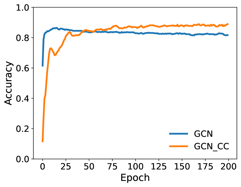
To evaluate the integration of ClassContrast (CC) with GNNs, we replace the initial node embeddings in GNNs with CC embeddings and assess their effectiveness. Accuracy results are presented in Table 4 and Figures 3 and 4 with additional details given in Appendix A. The results indicate that CC embeddings accelerate the convergence of GNN performance while maintaining a consistent accuracy gap over the vanilla model. Furthermore, combining CC with the recent LINKX model yields the best results across all baselines for both datasets, highlighting a promising avenue for enhancing GNN performance.

Table 4: Vanilla-GNN vs. GNN+CC accuracy results for node classification. See Appendix A for details.

Dataset	Model	GNN	CC-GNN	Imp.( $\uparrow$ )
CORA	GCN	86.14 $\pm$ 1.10	88.43 $\pm$ 0.92	2.29
	SAGE	86.26 $\pm$ 1.54	90.08 $\pm$ 1.37	3.82
	GAT	85.03 $\pm$ 1.61	87.18 $\pm$ 2.12	2.15
	LINKX	84.64 $\pm$ 1.13	90.06 $\pm$ 1.28	5.42
TEXAS	GCN	56.22 $\pm$ 5.81	70.81 $\pm$ 6.43	14.59
	SAGE	75.95 $\pm$ 5.01	87.84 $\pm$ 6.65	11.89
	GAT	54.32 $\pm$ 6.30	62.16 $\pm$ 5.70	7.84
	LINKX	74.60 $\pm$ 8.37	93.78 $\pm$ 4.04	19.18

Table 5: Link Prediction Performances. AUC results for Link Prediction. Baselines are reported from (Fu et al. 2023; Zhou et al. 2022). In the Overall column, we report mean AUC results across all datasets.

Dataset	CORA	CITESEER	PUBMED	WISC.	CORNELL	TEXAS	Overall
Node2vec (Grover et al. 2016)	0.856 $\pm$ 0.015	0.894 $\pm$ 0.014	0.919 $\pm$ 0.004	–	–	–	–
GAE (Kipf and Welling 2016)	0.895 $\pm$ 0.165	0.887 $\pm$ 0.084	0.957 $\pm$ 0.012	0.689 $\pm$ 0.384	0.736 $\pm$ 1.090	0.753 $\pm$ 1.297	0.820
VGAE (Kipf and Welling 2016)	0.852 $\pm$ 0.493	0.810 $\pm$ 0.339	0.929 $\pm$ 0.134	0.669 $\pm$ 0.866	0.783 $\pm$ 0.401	0.767 $\pm$ 0.557	0.802
ARVGE (Pan et al. 2018)	0.913 $\pm$ 0.079	0.878 $\pm$ 0.177	0.965 $\pm$ 0.015	0.711 $\pm$ 0.377	0.789 $\pm$ 0.501	0.765 $\pm$ 0.468	0.837
DGI (Veličković et al. 2018b)	0.898 $\pm$ 0.080	0.955 $\pm$ 0.100	0.912 $\pm$ 0.060	–	–	–	–
G-VAE (Grover et al. 2019)	0.947 $\pm$ 0.011	0.973 $\pm$ 0.006	0.974 $\pm$ 0.004	–	–	–	–
GNAE (Ahn and Kim 2021)	0.941 $\pm$ 0.063	0.969 $\pm$ 0.022	0.954 $\pm$ 0.019	0.782 $\pm$ 0.829	0.729 $\pm$ 1.083	0.751 $\pm$ 1.067	0.854
VGNAE (Ahn and Kim 2021)	0.892 $\pm$ 0.067	0.955 $\pm$ 0.055	0.897 $\pm$ 0.040	0.703 $\pm$ 0.120	0.733 $\pm$ 0.573	0.789 $\pm$ 0.302	0.828
GIC (Mavromatis et al. 2021)	0.935 $\pm$ 0.060	0.970 $\pm$ 0.050	0.937 $\pm$ 0.030	–	–	–	–
LINKX (Lim et al. 2021a)	0.934 $\pm$ 0.030	0.935 $\pm$ 0.050	–	0.801 $\pm$ 0.380	–	0.758 $\pm$ 0.470	0.857
DisenLink (Zhou et al. 2022)	0.971 $\pm$ 0.040	0.983 $\pm$ 0.030	–	0.844 $\pm$ 0.190	–	0.807 $\pm$ 0.400	0.901
DGAE (Fu et al. 2023)	0.958 $\pm$ 0.044	0.972 $\pm$ 0.034	0.978 $\pm$ 0.012	0.757 $\pm$ 0.586	0.681 $\pm$ 1.207	0.683 $\pm$ 1.279	0.838
VDGAE (Fu et al. 2023)	0.959 $\pm$ 0.042	0.978 $\pm$ 0.030	0.970 $\pm$ 0.012	0.850 $\pm$ 0.478	0.761 $\pm$ 0.475	0.813 $\pm$ 0.849	0.889
ClassContrast	0.967 $\pm$ 0.047	0.952 $\pm$ 0.059	0.980 $\pm$ 0.012	0.796 $\pm$ 0.338	0.814 $\pm$ 0.413	0.831 $\pm$ 0.393	0.905

Table 6: Homophily matrices for the SQUIRREL dataset. Every row represents the corresponding homophily ratio of the row’s class. In every row, the highest homophily ratio is marked bold.

ClassContrast Spatial-1 Homophily Matrix
	$\mathbf{C}_{1}$	$\mathbf{C}_{2}$	$\mathbf{C}_{3}$	$\mathbf{C}_{4}$	$\mathbf{C}_{5}$
$\mathbf{C}_{1}$	0.147	0.146	0.154	0.213	0.340
$\mathbf{C}_{2}$	0.132	0.162	0.173	0.221	0.312
$\mathbf{C}_{3}$	0.104	0.156	0.194	0.233	0.314
$\mathbf{C}_{4}$	0.106	0.146	0.176	0.252	0.320
$\mathbf{C}_{5}$	0.106	0.139	0.178	0.236	0.341

ClassContrast Spatial-2 Homophily Matrix
	$\mathbf{C}_{1}$	$\mathbf{C}_{2}$	$\mathbf{C}_{3}$	$\mathbf{C}_{4}$	$\mathbf{C}_{5}$
$\mathbf{C}_{1}$	0.167	0.170	0.197	0.229	0.236
$\mathbf{C}_{2}$	0.133	0.192	0.200	0.229	0.247
$\mathbf{C}_{3}$	0.121	0.168	0.236	0.226	0.250
$\mathbf{C}_{4}$	0.119	0.158	0.197	0.261	0.266
$\mathbf{C}_{5}$	0.118	0.152	0.193	0.230	0.307

ClassContrast Domain Homophily Matrix
	$\mathbf{C}_{1}$	$\mathbf{C}_{2}$	$\mathbf{C}_{3}$	$\mathbf{C}_{4}$	$\mathbf{C}_{5}$
$\mathbf{C}_{1}$	0.174	0.187	0.203	0.212	0.223
$\mathbf{C}_{2}$	0.164	0.194	0.205	0.214	0.224
$\mathbf{C}_{3}$	0.165	0.188	0.210	0.214	0.223
$\mathbf{C}_{4}$	0.162	0.187	0.205	0.220	0.226
$\mathbf{C}_{5}$	0.161	0.186	0.205	0.216	0.231

Table 7: Spatial vs. Contextual. Accuracy results of our model considering different feature subsets.

Features	CORA	CITESEER	PUBMED	TEXAS	CORNELL	WISC.	CHAM.	SQUIR.
Spatial Only	80.91 $\pm$ 1.64	60.63 $\pm$ 4.35	85.86 $\pm$ 0.32	67.29 $\pm$ 6.29	49.45 $\pm$ 4.23	57.84 $\pm$ 6.14	63.70 $\pm$ 3.05	44.67 $\pm$ 2.55
Context Only	83.13 $\pm$ 1.94	90.44 $\pm$ 1.27	89.70 $\pm$ 0.50	91.35 $\pm$ 4.37	92.71 $\pm$ 4.23	94.71 $\pm$ 2.62	78.81 $\pm$ 1.33	44.08 $\pm$ 1.58
Both (CC)	88.65 $\pm$ 1.25	86.86 $\pm$ 1.91	91.00 $\pm$ 0.45	90.54 $\pm$ 4.80	90.81 $\pm$ 2.90	93.33 $\pm$ 2.95	84.08 $\pm$ 1.55	54.65 $\pm$ 1.27

Ablation Study.

To evaluate the efficacy of our feature vectors, we conducted ablation studies for the node classification task. We employed three submodels: utilizing (1) spatial embeddings, (2) domain embeddings, and (3) both (ClassContrast embeddings). As given in Table 7, we observe that in the CORA, CHAMELEON, SQUIRREL, and PUBMED datasets, using only spatial or domain feature embeddings individually yields satisfactory performance. However, their combination significantly enhances performance in most cases. SQUIRREL ( $+10.57$ ) and CHAMELEON ( $+5.27$ ) experience a significant increase in accuracy in the combined setting. We note that when the ablation study has a large accuracy gap between the spatial and domain only models for a dataset (e.g., in TEXAS), the accuracies of the SOTA models in Table 2 show huge accuracy deviations for the dataset as well (e.g., TEXAS accuracies range from $54.32$ to $90.30$ ). A possible explanation is that models might individually capture either spatial or contextual information. Consequently, they may be unable to combine these two sets of features to counterbalance the insufficient information present in one of them, leading to diminished accuracy scores. In contrast, the ablation study offers evidence that the ClassContrast approach is resilient to this limitation and, experiences smaller accuracy losses (e.g., $91.35\rightarrow 90.54$ for TEXAS in Table 7).

5.2 Link Prediction Results

In this part, we show the utilization of ClassContrast Embeddings in the link prediction task. We utilize the common setting described in (Zhou et al. 2022) where the datasets were partitioned into training, validation, and test sets with a ratio of $85\%,5\%,$ and $10\%$ respectively.

The model architecture for the link prediction problem consists of three MLP layers. In this framework, for each considered node pairs $(u,v)$ , the normalized CC encodings are term-wise multiplied, $h_{u}\cdot h_{v}$ , and feed into MLP. We configure the model with a hidden neuron dimension of 16, a learning rate of 0.001, and train it over 100 epochs with a batch size of 128.

Table 5 reports the prediction results. We report the baselines from (Fu et al. 2023) and (Zhou et al. 2022), which use our experiment settings. Out of three homophilic and three heterophilic datasets, ClassContrast outperforms existing models in three datasets, and gets the second best result in one. On the six datasets, ClassContrast reaches the highest mean AUC of 0.905.

Limitations. The effectiveness of ClassContrast heavily depends on the quality and relevance of the landmarks used to define the contextual embeddings. If these are not representative of the actual data distributions, the model’s performance could be adversely affected. Moreover, the computational overhead associated with generating and processing these enhanced embeddings might be prohibitive for extremely large graphs or datasets with high-dimensional features.

6 Conclusion

In this work, we introduced ClassContrast, a novel method that integrates domain and spatial information from graphs. Our results show that ClassContrast effectively addresses the predictive limitations of using either spatial or domain information alone, yielding significant improvements when both feature sets are informative. Our computationally efficient model has outperformed or achieved highly competitive results compared to state-of-the-art GNNs across multiple graph tasks, including small/large and homophilic/heterophilic settings. For future work, we plan to extend the ClassContrast approach to effectively integrate with GNNs and to apply it to temporal graphs, incorporating both temporal information and node characteristics.

References

Abu-El-Haija et al. (2019) Abu-El-Haija, S.; Perozzi, B.; Kapoor, A.; Alipourfard, N.; Lerman, K.; Harutyunyan, H.; Ver Steeg, G.; and Galstyan, A. 2019. Mixhop: Higher-order graph convolutional architectures via sparsified neighborhood mixing. In international conference on machine learning, 21–29. PMLR.
Ahn and Kim (2021) Ahn, S. J.; and Kim, M. 2021. Variational graph normalized autoencoders. In Proceedings of the 30th ACM international conference on information & knowledge management, 2827–2831.
Arnold, Nallapati, and Cohen (2007) Arnold, A.; Nallapati, R.; and Cohen, W. W. 2007. A comparative study of methods for transductive transfer learning. In Seventh IEEE international conference on data mining workshops (ICDMW 2007), 77–82. IEEE.
Barceló et al. (2020) Barceló, P.; Kostylev, E. V.; Monet, M.; Pérez, J.; Reutter, J.; and Silva, J.-P. 2020. The logical expressiveness of graph neural networks. In 8th International Conference on Learning Representations (ICLR 2020).
Bodnar et al. (2022) Bodnar, C.; Di Giovanni, F.; Chamberlain, B.; Lio, P.; and Bronstein, M. 2022. Neural sheaf diffusion: A topological perspective on heterophily and oversmoothing in gnns. Advances in Neural Information Processing Systems, 35: 18527–18541.
Cartwright and Harary (1956) Cartwright, D.; and Harary, F. 1956. Structural balance: a generalization of Heider’s theory. Psychological review, 63(5): 277.
Chen, Ma, and Xiao (2018) Chen, J.; Ma, T.; and Xiao, C. 2018. FastGCN: Fast Learning with Graph Convolutional Networks via Importance Sampling. In International Conference on Learning Representations.
Chen et al. (2020) Chen, M.; Wei, Z.; Huang, Z.; Ding, B.; and Li, Y. 2020. Simple and deep graph convolutional networks. In International conference on machine learning, 1725–1735. PMLR.
Chien et al. (2020) Chien, E.; Peng, J.; Li, P.; and Milenkovic, O. 2020. Adaptive Universal Generalized PageRank Graph Neural Network. In International Conference on Learning Representations.
Ciano et al. (2021) Ciano, G.; Rossi, A.; Bianchini, M.; and Scarselli, F. 2021. On inductive–transductive learning with graph neural networks. IEEE Transactions on Pattern Analysis and Machine Intelligence, 44(2): 758–769.
Fu et al. (2023) Fu, J.; Zhang, X.; Li, S.; and Chen, D. 2023. Variational Disentangled Graph Auto-Encoders for Link Prediction. arXiv preprint arXiv:2306.11315.
Geng et al. (2021) Geng, Z.; Zhang, X.-Y.; Bai, S.; Wang, Y.; and Lin, Z. 2021. On training implicit models. NeurIPS, 34: 24247–24260.
Granovetter (1973) Granovetter, M. S. 1973. The strength of weak ties. American journal of sociology, 78(6): 1360–1380.
Grover et al. (2016) Grover, A.; et al. 2016. node2vec: Scalable feature learning for networks. In Proceedings of the 22nd ACM SIGKDD international conference on Knowledge discovery and data mining, 855–864.
Grover et al. (2019) Grover, A.; et al. 2019. Graphite: Iterative generative modeling of graphs. In International conference on machine learning, 2434–2444. PMLR.
Hamilton et al. (2017) Hamilton, W.; et al. 2017. Inductive representation learning on large graphs. NeurIPS, 30.
Haykin (1998) Haykin, S. 1998. Neural networks: a comprehensive foundation. Prentice Hall PTR.
Heider (1946) Heider, F. 1946. Attitudes and cognitive organization. The Journal of psychology, 21(1): 107–112.
Hu et al. (2020) Hu, W.; Fey, M.; Zitnik, M.; Dong, Y.; Ren, H.; Liu, B.; Catasta, M.; and Leskovec, J. 2020. Open graph benchmark: Datasets for machine learning on graphs. NeurIPS, 33: 22118–22133.
Huang et al. (2018) Huang, W.; Zhang, T.; Rong, Y.; and Huang, J. 2018. Adaptive sampling towards fast graph representation learning. NeurIPS, 31.
Jin et al. (2022) Jin, D.; Wang, R.; Ge, M.; He, D.; Li, X.; Lin, W.; and Zhang, W. 2022. RAW-GNN: RAndom Walk Aggregation based Graph Neural Network. In 31st International Joint Conference on Artificial Intelligence, IJCAI 2022, 2108–2114. International Joint Conferences on Artificial Intelligence.
Kipf and Welling (2016) Kipf, T. N.; and Welling, M. 2016. Variational graph auto-encoders. arXiv preprint arXiv:1611.07308.
Kipf and Welling (2017) Kipf, T. N.; and Welling, M. 2017. Semi-supervised classification with graph convolutional networks. ICLR.
Leskovec, Huttenlocher, and Kleinberg (2010) Leskovec, J.; Huttenlocher, D.; and Kleinberg, J. 2010. Signed networks in social media. In Proceedings of the SIGCHI conference on human factors in computing systems, 1361–1370.
Li et al. (2021) Li, G.; Müller, M.; Ghanem, B.; and Koltun, V. 2021. Training graph neural networks with 1000 layers. In International conference on machine learning, 6437–6449. PMLR.
Li et al. (2019) Li, G.; Muller, M.; Thabet, A.; and Ghanem, B. 2019. Deepgcns: Can gcns go as deep as cnns? In Proceedings of the IEEE/CVF international conference on computer vision, 9267–9276.
Li et al. (2022) Li, X.; Zhu, R.; Cheng, Y.; Shan, C.; Luo, S.; Li, D.; and Qian, W. 2022. Finding global homophily in graph neural networks when meeting heterophily. In International Conference on Machine Learning, 13242–13256. PMLR.
Liang et al. (2023) Liang, L.; Hu, X.; Xu, Z.; Song, Z.; and King, I. 2023. Predicting global label relationship matrix for graph neural networks under heterophily. Advances in Neural Information Processing Systems, 36.
Lim et al. (2021a) Lim, D.; Hohne, F.; Li, X.; Huang, S. L.; Gupta, V.; Bhalerao, O.; and Lim, S. N. 2021a. Large scale learning on non-homophilous graphs: New benchmarks and strong simple methods. NeurIPS, 34: 20887–20902.
Lim et al. (2021b) Lim, D.; Li, X.; Hohne, F.; and Lim, S.-N. 2021b. New benchmarks for learning on non-homophilous graphs. arXiv preprint arXiv:2104.01404.
Liu et al. (2022) Liu, J.; Hooi, B.; Kawaguchi, K.; and Xiao, X. 2022. Mgnni: Multiscale graph neural networks with implicit layers. NeurIPS, 35: 21358–21370.
Liu, Gao, and Ji (2020) Liu, M.; Gao, H.; and Ji, S. 2020. Towards deeper graph neural networks. In KDD, 338–348.
Liu, Wang, and Ji (2021) Liu, M.; Wang, Z.; and Ji, S. 2021. Non-local graph neural networks. IEEE transactions on pattern analysis and machine intelligence, 44(12): 10270–10276.
Luan et al. (2022) Luan, S.; Hua, C.; Lu, Q.; Zhu, J.; Zhao, M.; Zhang, S.; Chang, X.-W.; and Precup, D. 2022. Revisiting heterophily for graph neural networks. NeurIPS, 35: 1362–1375.
Luan et al. (2023) Luan, S.; Hua, C.; Xu, M.; Lu, Q.; Zhu, J.; Chang, X.-W.; Fu, J.; Leskovec, J.; and Precup, D. 2023. When do graph neural networks help with node classification: Investigating the homophily principle on node distinguishability. NeurIPS.
Mavromatis et al. (2021) Mavromatis, C.; et al. 2021. Graph infoclust: Maximizing coarse-grain mutual information in graphs. In Pacific-Asia Conference on Knowledge Discovery and Data Mining, 541–553. Springer.
Mikolov et al. (2013a) Mikolov, T.; Chen, K.; Corrado, G.; and Dean, J. 2013a. Efficient estimation of word representations in vector space. arXiv preprint arXiv:1301.3781.
Mikolov et al. (2013b) Mikolov, T.; Sutskever, I.; Chen, K.; Corrado, G. S.; and Dean, J. 2013b. Distributed representations of words and phrases and their compositionality. NeurIPS, 26.
Mislove et al. (2007) Mislove, A.; Marcon, M.; Gummadi, K. P.; Druschel, P.; and Bhattacharjee, B. 2007. Measurement and analysis of online social networks. In Proceedings of the 7th ACM SIGCOMM conference on Internet measurement, 29–42.
Morris et al. (2019) Morris, C.; Ritzert, M.; Fey, M.; Hamilton, W. L.; Lenssen, J. E.; Rattan, G.; and Grohe, M. 2019. Weisfeiler and leman go neural: Higher-order graph neural networks. In Proceedings of the AAAI conference on artificial intelligence, volume 33-01, 4602–4609.
Niwattanakul et al. (2013) Niwattanakul, S.; Singthongchai, J.; Naenudorn, E.; and Wanapu, S. 2013. Using of Jaccard coefficient for keywords similarity. In Proceedings of the international multiconference of engineers and computer scientists, volume 1, 380–384.
Oono and Suzuki (2020) Oono, K.; and Suzuki, T. 2020. Graph Neural Networks Exponentially Lose Expressive Power for Node Classification. In International Conference on Learning Representations.
Pan et al. (2018) Pan, S.; Hu, R.; Long, G.; Jiang, J.; Yao, L.; and Zhang, C. 2018. Adversarially regularized graph autoencoder for graph embedding. arXiv preprint arXiv:1802.04407.
Pei et al. (2019) Pei, H.; Wei, B.; Chang, K. C.-C.; Lei, Y.; and Yang, B. 2019. Geom-GCN: Geometric Graph Convolutional Networks. In International Conference on Learning Representations.
Platonov et al. (2023) Platonov, O.; Kuznedelev, D.; Babenko, A.; and Prokhorenkova, L. 2023. Characterizing graph datasets for node classification: Homophily-heterophily dichotomy and beyond. Advances in Neural Information Processing Systems, 36.
Plotkin and Onuchic (2002) Plotkin, S. S.; and Onuchic, J. N. 2002. Understanding protein folding with energy landscape theory part I: basic concepts. Quarterly reviews of biophysics, 35(2): 111–167.
Sen et al. (2008) Sen, P.; Namata, G.; Bilgic, M.; Getoor, L.; Galligher, B.; and Eliassi-Rad, T. 2008. Collective classification in network data. AI Magazine, 29(3): 93–93.
Shervashidze et al. (2011) Shervashidze, N.; Schweitzer, P.; Van Leeuwen, E. J.; Mehlhorn, K.; and Borgwardt, K. M. 2011. Weisfeiler-lehman graph kernels. JMLR, 12(9).
Shi et al. (2020) Shi, Y.; Huang, Z.; Feng, S.; Zhong, H.; Wang, W.; and Sun, Y. 2020. Masked label prediction: Unified message passing model for semi-supervised classification. arXiv preprint arXiv:2009.03509.
Suresh et al. (2021) Suresh, S.; Budde, V.; Neville, J.; Li, P.; and Ma, J. 2021. Breaking the limit of graph neural networks by improving the assortativity of graphs with local mixing patterns. In Proceedings of the 27th ACM SIGKDD Conference on Knowledge Discovery & Data Mining, 1541–1551.
Tang et al. (2008) Tang, J.; Zhang, J.; Yao, L.; Li, J.; Zhang, L.; and Su, Z. 2008. Arnetminer: extraction and mining of academic social networks. In Proceedings of the 14th ACM SIGKDD international conference on Knowledge discovery and data mining, 990–998.
Topping et al. (2021) Topping, J.; Di Giovanni, F.; Chamberlain, B. P.; Dong, X.; and Bronstein, M. M. 2021. Understanding over-squashing and bottlenecks on graphs via curvature. arXiv preprint arXiv:2111.14522.
Veličković et al. (2018a) Veličković, P.; Cucurull, G.; Casanova, A.; Romero, A.; Lio, P.; and Bengio, Y. 2018a. Graph attention networks. ICLR.
Veličković et al. (2018b) Veličković, P.; Fedus, W.; Hamilton, W. L.; Liò, P.; Bengio, Y.; and Hjelm, R. D. 2018b. Deep graph infomax. arXiv preprint arXiv:1809.10341.
Wales (2002) Wales, D. J. 2002. Energy landscapes. In Atomic clusters and nanoparticles. Agregats atomiques et nanoparticules: Les Houches Session LXXIII 2–28 July 2000, 437–507. Springer.
Wales et al. (1998) Wales, D. J.; et al. 1998. Archetypal energy landscapes. Nature, 394(6695): 758–760.
Wang et al. (2020) Wang, K.; Shen, Z.; Huang, C.; Wu, C.-H.; Dong, Y.; and Kanakia, A. 2020. Microsoft academic graph: When experts are not enough. Quantitative Science Studies, 1(1): 396–413.
Xiao et al. (2022) Xiao, S.; Wang, S.; Dai, Y.; and Guo, W. 2022. Graph neural networks in node classification: survey and evaluation. Machine Vision and Applications, 33: 1–19.
Xu et al. (2019) Xu, K.; Hu, W.; Leskovec, J.; and Jegelka, S. 2019. How Powerful are Graph Neural Networks? In International Conference on Learning Representations.
Xu et al. (2023) Xu, Z.; Chen, Y.; Zhou, Q.; Wu, Y.; Pan, M.; Yang, H.; and Tong, H. 2023. Node classification beyond homophily: Towards a general solution. In Proceedings of the 29th ACM SIGKDD Conference on Knowledge Discovery and Data Mining, 2862–2873.
Yan et al. (2022) Yan, Y.; Hashemi, M.; Swersky, K.; Yang, Y.; and Koutra, D. 2022. Two sides of the same coin: Heterophily and oversmoothing in graph convolutional neural networks. In 2022 IEEE International Conference on Data Mining (ICDM), 1287–1292. IEEE.
Yu et al. (2022a) Yu, L.; Sun, L.; Du, B.; Liu, C.; Lv, W.; and Xiong, H. 2022a. Heterogeneous graph representation learning with relation awareness. IEEE Transactions on Knowledge and Data Engineering.
Yu et al. (2022b) Yu, L.; Sun, L.; Du, B.; Zhu, T.; and Lv, W. 2022b. Label-Enhanced Graph Neural Network for Semi-supervised Node Classification. IEEE Transactions on Knowledge and Data Engineering.
Zhang et al. (2022) Zhang, L.; Song, H.; Aletras, N.; and Lu, H. 2022. Node-feature convolution for graph convolutional networks. Pattern Recognition, 128: 108661.
Zheng et al. (2022) Zheng, X.; Liu, Y.; Pan, S.; Zhang, M.; Jin, D.; and Yu, P. S. 2022. Graph neural networks for graphs with heterophily: A survey. arXiv preprint arXiv:2202.07082.
Zhou et al. (2022) Zhou, S.; Guo, Z.; Aggarwal, C.; Zhang, X.; and Wang, S. 2022. Link prediction on heterophilic graphs via disentangled representation learning. arXiv preprint arXiv:2208.01820.
Zhu et al. (2020) Zhu, J.; Yan, Y.; Zhao, L.; Heimann, M.; Akoglu, L.; and Koutra, D. 2020. Beyond homophily in graph neural networks: Current limitations and effective designs. NeurIPS, 33: 7793–7804.

Appendix

Appendix A Integrating ClassContrast with GNNs

While our primary goal is to develop an approach that synergistically combines spatial and contextual information, we also conducted additional experiments to evaluate how well the ClassContrast features integrate with existing GNN models. In particular, we tested the three classical GNN models, namely GCN, GraphSAGE and GAT, as well as the recent model LINKX. We replaced the node features as initial node embeddings in original GNN models with our ClassContrast features. We implemented a two-layer GNN framework using the Adam optimizer with an initial learning rate of 0.05. The hyperparameters include a dropout rate of 0.5, a weight decay of 5e-4, and 32 hidden channels. The results presented in Figure 3 and Table 4 indicate a noteworthy improvement in GNN performance when utilizing ClassContrast vectors. This enhancement is attributed to the effective embeddings provided by ClassContrast vectors. Furthermore, the observed accuracy gap remains stable. In our future endeavors, we plan to delve deeper into this direction for a more comprehensive exploration.

Appendix B Heterophily and ClassContrast

B.1 Recent Homophily Metrics

Until recently, the prevailing homophily metrics were node homophily (Pei et al. 2019) and edge homophily (Abu-El-Haija et al. 2019; Zhu et al. 2020). Node homophily simply computes, for each node, the proportion of its neighbors that belong to the same class, and averages across all nodes, while edge homophily measures the proportion of edges connecting nodes of the same class compared to all edges in the network. In the past few years, to study heterophily phenomena in graph representation learning, several new homophily metrics were introduced, e.g., class homophily (Lim et al. 2021b), generalized edge homophily (Jin et al. 2022) and aggregation homophily (Luan et al. 2022), adjusted homophily (Platonov et al. 2023) and label informativeness (Platonov et al. 2023). In Table 8, we give these metrics for our datasets. The details of these metrics can be found in (Luan et al. 2023).

Table 8: Homophily metrics for our datasets.

Metric	CORA	CITES.	PUBMED	TEXAS	CORNELL	WISC.	CHAM.	SQUIR.
$\mathcal{H}_{CC}$ -spat-1	0.8129	0.6861	0.7766	0.1079	0.1844	0.2125	0.2549	0.2564
$\mathcal{H}_{CC}$ -context	0.1702	0.1949	0.3245	0.2352	0.2409	0.2449	0.2564	0.2057
$\mathcal{H}_{\text{node}}$	0.8252	0.7175	0.7924	0.3855	0.1498	0.0968	0.2470	0.2156
$\mathcal{H}_{\text{edge}}$	0.8100	0.7362	0.8024	0.5669	0.4480	0.4106	0.2795	0.2416
$\mathcal{H}_{\text{class}}$	0.7657	0.6270	0.6641	0.0468	0.0941	0.0013	0.0620	0.0254
$\mathcal{H}_{\text{agg}}$	0.9904	0.9826	0.9432	0.8032	0.7768	0.6940	0.6100	0.3566
$\mathcal{H}_{\text{GE}}$	0.1700	0.1900	0.2700	0.3100	0.3400	0.3500	0.0152	0.0157
$\mathcal{H}_{\text{adj}}$	0.8178	0.7588	0.7431	0.1889	0.0826	0.0258	0.0663	0.0196
LI	0.5904	0.4508	0.4093	0.0169	0.1311	0.1923	0.0480	0.0015

Table 9: Homophily matrices for CORA dataset. Every row represents the corresponding homophily ratio of the row’s class. In every row, the highest homophily ratio is marked bold.

ClassContrast Spatial-1 Homophily Matrix
	$\mathbf{C}_{1}$	$\mathbf{C}_{2}$	$\mathbf{C}_{3}$	$\mathbf{C}_{4}$	$\mathbf{C}_{5}$	$\mathbf{C}_{6}$	$\mathbf{C}_{7}$
$\mathbf{C}_{1}$	0.743	0.029	0.014	0.083	0.050	0.037	0.043
$\mathbf{C}_{2}$	0.040	0.769	0.062	0.080	0.020	0.028	0.002
$\mathbf{C}_{3}$	0.010	0.025	0.917	0.032	0.001	0.014	0.001
$\mathbf{C}_{4}$	0.055	0.020	0.016	0.839	0.051	0.015	0.004
$\mathbf{C}_{5}$	0.058	0.014	0.002	0.064	0.849	0.011	0.003
$\mathbf{C}_{6}$	0.058	0.017	0.030	0.051	0.018	0.786	0.040
$\mathbf{C}_{7}$	0.113	0.001	0.003	0.022	0.006	0.067	0.788

ClassContrast Context-S Homophily Matrix
	$\mathbf{C}_{1}$	$\mathbf{C}_{2}$	$\mathbf{C}_{3}$	$\mathbf{C}_{4}$	$\mathbf{C}_{5}$	$\mathbf{C}_{6}$	$\mathbf{C}_{7}$
$\mathbf{C}_{1}$	0.206	0.143	0.126	0.111	0.124	0.143	0.147
$\mathbf{C}_{2}$	0.123	0.236	0.146	0.121	0.101	0.147	0.126
$\mathbf{C}_{3}$	0.109	0.171	0.253	0.107	0.088	0.136	0.137
$\mathbf{C}_{4}$	0.122	0.170	0.168	0.159	0.130	0.134	0.118
$\mathbf{C}_{5}$	0.130	0.154	0.118	0.110	0.240	0.137	0.111
$\mathbf{C}_{6}$	0.112	0.148	0.135	0.103	0.078	0.283	0.142
$\mathbf{C}_{7}$	0.150	0.146	0.123	0.093	0.097	0.154	0.236

ClassContrast Context-I Homophily Matrix
	$\mathbf{C}_{1}$	$\mathbf{C}_{2}$	$\mathbf{C}_{3}$	$\mathbf{C}_{4}$	$\mathbf{C}_{5}$	$\mathbf{C}_{6}$	$\mathbf{C}_{7}$
$\mathbf{C}_{1}$	0.159	0.134	0.142	0.154	0.143	0.136	0.132
$\mathbf{C}_{2}$	0.142	0.159	0.146	0.154	0.139	0.138	0.122
$\mathbf{C}_{3}$	0.136	0.140	0.162	0.156	0.140	0.138	0.127
$\mathbf{C}_{4}$	0.145	0.136	0.146	0.168	0.151	0.133	0.122
$\mathbf{C}_{5}$	0.144	0.131	0.144	0.159	0.167	0.133	0.124
$\mathbf{C}_{6}$	0.142	0.132	0.145	0.149	0.145	0.158	0.129
$\mathbf{C}_{7}$	0.142	0.126	0.142	0.152	0.141	0.138	0.159

Table 10: Homophily matrices for the WISCONSIN dataset. Every row represents the corresponding homophily ratio of the row’s class. In every row, the highest homophily ratio is marked bold.

ClassContrast Spatial-1 Homophily Matrix
	$\mathbf{C}_{1}$	$\mathbf{C}_{2}$	$\mathbf{C}_{3}$	$\mathbf{C}_{4}$	$\mathbf{C}_{5}$
$\mathbf{C}_{1}$	0.323	0.000	0.000	0.323	0.323
$\mathbf{C}_{2}$	0.001	0.219	0.595	0.185	0.001
$\mathbf{C}_{3}$	0.000	0.547	0.225	0.145	0.084
$\mathbf{C}_{4}$	0.044	0.268	0.468	0.071	0.150
$\mathbf{C}_{5}$	0.149	0.039	0.397	0.200	0.215

ClassContrast Spatial-2 Homophily Matrix
	$\mathbf{C}_{1}$	$\mathbf{C}_{2}$	$\mathbf{C}_{3}$	$\mathbf{C}_{4}$	$\mathbf{C}_{5}$
$\mathbf{C}_{1}$	0.444	0.278	0.111	0.111	0.056
$\mathbf{C}_{2}$	0.001	0.439	0.438	0.106	0.016
$\mathbf{C}_{3}$	0.011	0.351	0.481	0.111	0.046
$\mathbf{C}_{4}$	0.029	0.238	0.485	0.110	0.138
$\mathbf{C}_{5}$	0.149	0.084	0.374	0.136	0.258

ClassContrast Domain Homophily Matrix
	$\mathbf{C}_{1}$	$\mathbf{C}_{2}$	$\mathbf{C}_{3}$	$\mathbf{C}_{4}$	$\mathbf{C}_{5}$
$\mathbf{C}_{1}$	0.221	0.198	0.207	0.192	0.181
$\mathbf{C}_{2}$	0.148	0.247	0.223	0.201	0.181
$\mathbf{C}_{3}$	0.174	0.205	0.228	0.204	0.189
$\mathbf{C}_{4}$	0.145	0.203	0.217	0.237	0.199
$\mathbf{C}_{5}$	0.149	0.204	0.209	0.209	0.230


	$\displaystyle\mathcal{H}_{\text{edge}}(\mathcal{G})=\frac{\big{\|}\{e_{uv}\mid e_{uv}\in\mathcal{E},Z_{u,:}=Z_{v,:}\}\big{\|}}{\|\mathcal{E}\|}$
	$\displaystyle\mathcal{H}_{\text{class}}(\mathcal{G})\!=\!\frac{1}{C\!-\!1}\sum_{k=1}^{C}\bigg{[}h_{k}\!-\!\frac{\big{\|}\{v\mid Z_{v,k}\!=\!1\}\big{\|}}{N}\bigg{]}_{+}$
	$\displaystyle\text{where }h_{k}\!=\!\frac{\sum_{v\in\mathcal{V},Z_{v,k}=1}\big{\|}\{u\mid u\in\mathcal{N}_{v},Z_{u,:}\!=\!Z_{v,:}\}\big{\|}}{\sum_{v\in\{v\|Z_{v,k}=1\}}d_{v}}$
	$\displaystyle\mathcal{H}_{\text{GE}}(\mathcal{G})=\frac{\sum\limits_{(i,j)\in\mathcal{E}}\text{cos}(x_{i},x_{j})}{\|\mathcal{E}\|}$

	$\displaystyle\mathcal{H}_{\text{adj}}=\frac{\mathcal{H}_{\text{edge}}-\sum_{c=1}^{C}\bar{p}_{c}^{2}}{1-\sum_{k=1}^{C}\bar{p}_{c}^{2}}$

where $\mathcal{H}_{\text{node}}^{v}$ is the local homophily value for node $v$ ; $[a]_{+}=\max(0,a)$ ; $h_{k}$ is the class-wise homophily metric (Lim et al. 2021b); $\mathrm{Mean}_{u}\left(\{\cdot\}\right)$ takes the average over $u$ of a given multiset of values or variables and $S(\hat{A},Z)=\hat{A}Z(\hat{A}Z)^{\top}$ is the post-aggregation node similarity matrix; $D_{c}=\sum_{v:z_{v}=c}d_{v},\bar{p}_{c}=\frac{D_{c}}{2|\mathcal{E}|}$ , $p_{c_{1},c_{2}}=\sum_{(u,v)\in\mathcal{E}}\frac{1\{z_{u}=c_{1},z_{v}=c_{2}\}}{2|\mathcal{E}|},c,c_{1},c_{2}\in\{1,\dots,C\}$ .

In Table 9 below, we give ClassContrast Homophily matrices which provides detailed insights on the class interactions in CORA dataset. In particular, Spatial-1 matrix interprets as for any class, the nodes likely to form a link with same class node in their one neighborhood. In the following Contextual-Selective and Contextual-Inclusive Homophily matrices, independent of graph distance, we see the positions of attribute vectors similarity to the chosen class landmarks.

B.2 ClassContrast Homophily Matrices

We provide further homophily matrices for one homophilic and one heterophilic graphs. In Table 9, for CORA dataset, we observe in CC Spatial-1, Context-S and Context-I Homophily matrices show the strong homophily behavior in both spatial and contextual aspects. In Spatial-1 matrix the entry $h_{ij}$ represents how likely the nodes in $\mathcal{C}_{i}$ to connect to nodes in $\mathcal{C}_{j}$ among their $1$ -neighborhood. The very high numbers in the diagonal shows that most classes likely to connect with their own class, as CORA’s node homophily ratio (0.83) suggest. From the matrix, we have finer information that the class $\mathcal{C}_{3}$ is very highly homophilic. The domain matrices represents the average similarity/closeness to class landmarks. We observe that in both domain matrices, the node feature vectors likely to land close to their own class landmark, and ClassContrast vectors captures this crucial information.

In Table 10, for WISCONSIN dataset, spatial-1 and Spatial-2 matrices show the irregular behavior as the WISCONSIN node homophily ratio (0.09) suggest. The nodes are unlikely to connect their adjacent nodes in the same class. Even in their two neighborhoods, they don’t have many of their fellow classmate for $\mathcal{C}_{4}$ and $\mathcal{C}_{5}$ . However, while the other three classes are not connecting their own classmate, they have several common neighbors. Finally, the domain homophily matrix again shows that while they are not very close in the graph, they all share common interests, as every node’s feature vector lands close to their classmates’.

While different homophily ratios are summarizing crucial information about node tendencies, we observe that our matrices are giving much finer and easily intepretable information no class behaviors.

B.3 Proof of the Theorem and New Homophily Metrics

In Section 4.4, we have defined homophily and discussed the relation between ClassContrast vectors and the homophily notion. Here we give details how to generalize this idea to give finer homophily notions for graphs. First, we give the proof of Theorem 4.7.

Theorem B.1.

For an undirected graph $\mathcal{G}=(\mathcal{V},\mathcal{E})$ , let $\vec{\alpha}_{1}(v)$ be the spatial vector defined in Appendix B. Let $\widehat{\alpha}_{1}(v)$ be the vector where the entry corresponding to class of $v$ is set to $0$ . Then,

1-\varphi(\mathcal{G})=\frac{1}{|\mathcal{V}|}\sum_{v\in\mathcal{V}}\frac{\|\widehat{\alpha}_{1}(v)\|_{1}}{\|\vec{\alpha}_{1}(v)\|_{1}}

Proof.

For an undirected graph $\mathcal{G}=(\mathcal{V},\mathcal{E})$ with node class assignment function $\mathcal{C}:\mathcal{V}\to\{1,2,\dots,N\}$ , $\vec{\alpha}_{1}(v)=[a_{1}(v)\ a_{2}(v)\ \dots\ a_{N}(v)]$ where $a_{i}(v)=\#\{u\in\mathcal{N}_{1}(v)\mid\mathcal{C}(u)=i\}$ . Let $\mathcal{C}(v)=j_{v}$ . Then, by setting $a_{j_{v}}(v)=0$ , we get a new vector $\widehat{\alpha}_{1}(v)=[a_{1}(v)\dots\ a_{j_{v}-1}(v)\ 0\ a_{j_{v}+1}(v)\ \dots]$

$L^{1}$ -norm of $\vec{\alpha}_{1}(v)$ is $\|\vec{\alpha}_{1}(v)\|_{1}=\sum_{i=1}^{N}a_{i}(v)$ . Similarly, $\|\widehat{\alpha}_{1}(v)\|_{1}=\sum_{i\neq j_{v}}a_{i}(v)$ . Hence, we have $\|\vec{\alpha}_{1}(v)\|_{1}-\|\widehat{\alpha}_{1}(v)\|_{1}=a_{j_{v}}(v)$ . Notice that by definition, $a_{j_{v}}(v)=\eta(v)$ , the number of neighbors in the same class with $v$ . Similarly, $\|\vec{\alpha}_{1}(v)\|_{1}=deg(v)$ . Hence,

1-\dfrac{\|\widehat{\alpha}_{1}(v)\|_{1}}{\|\vec{\alpha}_{1}(v)\|_{1}}=\dfrac{\|\vec{\alpha}_{1}(v)\|_{1}-\|\widehat{\alpha}_{1}(v)\|_{1}}{\|\vec{\alpha}_{1}(v)\|_{1}}=\dfrac{\eta(v)}{deg(v)}

(1)

As $\varphi(\mathcal{G})=\dfrac{1}{|\mathcal{V}|}\sum_{v\in\mathcal{V}}\dfrac{\eta(v)}{deg(v)}$ , we have $1-\varphi(\mathcal{G})$ as

1-\frac{1}{|\mathcal{V}|}\sum_{v\in\mathcal{V}}\frac{\eta(v)}{deg(v)}=\frac{1}{|\mathcal{V}|}\sum_{v\in\mathcal{V}}(1-\frac{\eta(v)}{deg(v)})=\frac{1}{|\mathcal{V}|}\sum_{v\in\mathcal{V}}\frac{\|\widehat{\alpha}_{1}(v)\|_{1}}{\|\vec{\alpha}_{1}(v)\|_{1}}

where the last equality follows by Equation 1. The proof follows. ∎

This perspective inspires different ways to generalize the homophily concept by using ClassContrast vectors. Notice that in ClassContrast matrices above, we employed a classwise grouping to measure class interactions. If we do not use any grouping for the nodes, we get natural generalizations of existing homophily ratios. First, we define higher homophily by using the ratio of the number of nodes in the $2$ -neighborhood $\mathcal{N}_{2}(v)$ with the same class to $|\mathcal{N}_{2}(v)|$ .

Definition B.2 (Higher Homophily).

Given $\mathcal{G}=(\mathcal{V},\mathcal{E})$ with $\mathcal{C}:\mathcal{V}\to\{1,2,\dots,N\}$ representing node classes. Let $\eta_{2}(v)$ be the number of nodes in $\mathcal{N}_{2}(v)$ in the same class with $v$ . Then, homophily ratio of $\mathcal{G}$ is defined as

\varphi_{2}(\mathcal{G})=\frac{1}{|\mathcal{V}|}\sum_{v\in\mathcal{V}}\frac{\eta_{2}(v)}{|\mathcal{N}_{2}(v)|}

By applying similar ideas to the proof of Theorem 4.7, we obtain the following result.

Theorem B.3.

For an undirected graph $\mathcal{G}=(\mathcal{V},\mathcal{E})$ , let $\vec{\alpha}_{2}(v)$ be the spatial vector defined above. Let $\widehat{\alpha}_{2}(v)$ be the vector where the entry corresponding to the class of $v$ is set to $0$ . Then,

1-\varphi_{2}(\mathcal{G})=\frac{1}{|\mathcal{V}|}\sum_{v\in\mathcal{V}}\frac{\|\widehat{\alpha}_{2}(v)\|_{1}}{\|\vec{\alpha}_{2}(v)\|_{1}}

While the above notions represent structural homophily, we introduce another homophily by comparing the contextual vectors of neighboring nodes with the central node’s.

Definition B.4 (Contextual Homophily).

Given $\mathcal{G}=(\mathcal{V},\mathcal{E})$ with $\mathcal{C}:\mathcal{V}\to\{1,2,\dots,N\}$ representing node classes. Let $\vec{\beta}(v)$ be the contextual vector as defined in Section 4.2. Let $\widehat{\beta}(v)$ be the vector where the entry corresponding to the class of $v$ is set to $0$ .Then, define the contextual homophily of $\mathcal{G}$ as

\varphi_{\mathcal{D}}(\mathcal{G})=1-\frac{1}{|\mathcal{V}|}\sum_{v\in\mathcal{V}}\frac{\|\widehat{\beta}(v)\|_{1}}{\|\vec{\beta}(v)\|_{1}}

Similar homophily metrics, as introduced in (Luan et al. 2023; Lim et al. 2021b; Zhu et al. 2020; Jin et al. 2022), were employed to investigate the concept of heterophily in graph representation learning. In particular, our ClassContrast features inherently encompass this information, enabling the ML classifier to adapt accordingly. This explains the outstanding performance of ClassContrast in both homophilic and heterophilic settings for node classification and link prediction.

Appendix C Generalizations of ClassContrast

C.1 Inductive and Transductive Settings

Inductive Setting. In the inductive learning framework, a model is trained by using the training data $\mathcal{D}_{train}$ while the test data, $\mathcal{D}_{test}$ is completely hidden during the training time. This means that no information about test nodes (e.g., edges between training and test nodes) is provided during the training stage. The learning procedure aims to minimize a suitable loss function to capture the statistical distribution of the training data. Once an inductive model has undergone training, it can be utilized to make predictions on new (unseen) data, thereby determining the labels for unlabeled nodes.

Transductive Setting. In the transductive learning framework, which closely aligns with semi-supervised learning, both the training data $\mathcal{D}_{train}$ and the test data $\mathcal{D}_{test}$ can be simultaneously leveraged to capitalize on their interconnectedness. This interrelationship can be employed either during the training phase, the prediction phase, or both. Specifically, in the training stage, the information about $v_{test}$ and its position in the graph is known, while its label $y_{test}$ remains concealed. Consequently, the model is trained with explicit awareness of the nodes it will be evaluated on after the training process. This can serve as a valuable asset for the model, enabling it to establish a sound decision function by exploiting the characteristics observed in $v_{test}$ .

To clarify the differences between the inductive and transductive settings in graph-based learning, consider a given graph $\mathcal{G}$ , with datasets $\mathcal{D}_{\text{train}}$ and $\mathcal{D}_{\text{test}}$ . In the inductive setting, all test nodes and their connected edges are removed to create the training subgraph $\mathcal{G}_{\text{train}}$ . The model is trained exclusively on $\mathcal{G}_{\text{train}}$ and only gains access to the complete graph $\mathcal{G}$ during the testing stage. Conversely, in the transductive learning approach, the model has access to the entire graph $\mathcal{G}$ during training; however, the labels of the test nodes remain hidden throughout this process. It is noteworthy that any dataset configured for transductive learning can be adapted to the inductive setting by excluding test nodes and their connecting edges during the training phase. However, converting from the inductive to the transductive setting is not generally feasible. For further details, see the references (Ciano et al. 2021; Arnold, Nallapati, and Cohen 2007).

C.2 ClassContrast for Transductive Setting and Iterated Predictions

So far, we outlined our ClassContrast vectors for simplicity in inductive setting. To adapt to the transductive setting, we make adjustments without altering contextual vectors. In transductive setting, test node labels are hidden during training, but connection information to training nodes is available. We introduce a new "unknown" class $\mathcal{C}_{u}$ for test nodes with unknown labels, considering them as neighbors to training nodes. Each node $u\in\mathcal{V}$ is represented by a $N+1$ dimensional vector $\vec{\alpha}^{0}_{1}(u)=[a^{0}_{10}\ \ a^{0}_{11}\ \ a^{0}_{12}\ \ \dots\ \ a^{0}_{1N}]$ , where $a^{0}_{10}$ is the count of neighboring test nodes (unknown labels) of node $u$ , and $a^{0}_{1j}$ is the count of neighboring training nodes in class $\mathcal{C}_{j}$ for $1\leq j\leq N$ . Similar representations are defined for $\vec{\alpha}_{1i}(u)$ , $\vec{\alpha}_{1o}(u)$ , and $\vec{\alpha}_{2}(u)$ . The superscript $0$ indicates no iterations have occurred yet.

Iterated Predictions: Recall that the ultimate goal in the node classification problem is to predict the labels of new (test) nodes. After we obtain all ClassContrast vectors for training and test nodes above, we let our ML model make a prediction for each test node $v\in\mathcal{V}_{test}$ . Let $\mathcal{P}_{0}:\mathcal{V}_{test}\to\{\mathcal{C}_{1},\dots,\mathcal{C}_{N}\}$ be our predictions. Hence, we have a label for each node in our graph $\mathcal{G}$ .

While the original spatial vector $\vec{\alpha}^{0}_{1}(u)$ cannot use any class information for the test nodes, in the next step, we remedy this by using our class predictions for test nodes. In particular, by using the predictions $\mathcal{P}_{0}$ , we define a new (improved) spatial vector $\vec{\alpha}^{1}_{1}(u)=[a^{1}_{11}\ \ a^{1}_{12}\ \ a^{1}_{13}\ \ \dots\ \ a^{1}_{1N}]$ where we use predictions $\mathcal{P}_{0}$ for neighboring test nodes. Notice that this is no longer a $(N+1)$ -dimensional vector as there is no unknown class anymore. Similarly, we update all spatial vectors, train our ML model with these new node labels, and make a new prediction for test nodes. Then, we get new label predictions $\mathcal{P}_{1}:\mathcal{V}_{test}\to\{\mathcal{C}_{1},\dots,\mathcal{C}_{N}\}$ . By using predictions $\mathcal{P}_{1}$ , we define the next iteration $\vec{\alpha}^{2}_{1}(u)=[a^{2}_{11}\ \ a^{2}_{12}\ \ \dots\ \ a^{2}_{1N}]$ and train our model with these updated vectors. Again, we get new predictions $\mathcal{P}_{2}:\mathcal{V}_{test}\to\{\mathcal{C}_{1},\dots,\mathcal{C}_{N}\}$ . In our experiments, we observe that $1$ or $2$ iterations ( $\mathcal{P}_{1}$ or $\mathcal{P}_{2}$ ) improve the performance significantly, but further iterations do not, in the transductive setting.

C.3 Spatial Embeddings on Directed, Weighted Graphs

Directed Graphs. When $\mathcal{G}$ is directed, to obtain finer information about node neighborhoods, we produce two different embeddings of size $N$ , $\vec{\alpha}_{ki}(u)$ and $\vec{\alpha}_{ko}(u)$ for the k-hop neighborhood:

\vec{\alpha}_{ki}(u)=[a^{i}_{k1}\ \ a^{i}_{k2}\ \ \dots\ \ a^{i}_{kN}]\quad\vec{\alpha}_{ko}(u)=[a^{o}_{k1}\ \ a^{o}_{k2}\ \ \dots\ \ a^{o}_{kN}]

where $a^{i}_{kj}$ is the count of k-hop neighbors incoming to $u$ belonging to class $\mathcal{C}_{j}$ while $a^{o}_{kj}$ is the count of neighbors outgoing from $u$ belonging to class $\mathcal{C}_{j}$ (See Figure 2(a)).

Weighted Graphs: In weighted graphs, the counts incorporate edge weight information. Specifically, we define the weighted feature vector $\vec{\alpha}^{w}_{k}(u)$ for node $u$ as: $\vec{\alpha}^{w}_{k}(u)=[a^{w}_{k1},a^{w}_{k2},a^{w}_{k3},\dots,a^{w}_{kN}]$ where $a^{w}_{kj}$ is the sum of the weights of the edges connecting $u$ to the $k$ -hop neighbors belonging to class $\mathcal{C}_{j}$ . If the weight of an edge is inversely proportional to the similarity between nodes, one can use the sum of the reciprocals of the weights instead: $a^{w}_{kj}=\sum_{v\in\mathcal{N}_{k}(u)\cap\mathcal{C}_{j}}\frac{1}{\text{weight}(u,v)}$ . This approach allows for adjustments in how edge weights influence the calculation of proximity and class association. Additionally, in the context of directed graphs within a weighted graph setting, different vectors can be defined for incoming and outgoing neighborhood connections, such as $\vec{\alpha}^{w}_{ki}(u)$ for incoming edges and $\vec{\alpha}^{w}_{ko}(u)$ for outgoing edges, providing a more detailed representation of node relationships based on directionality and weight.

Table 11: The dimension of the ClassContrast embedding used for each dataset in our model

	CORA	CITESEER	PUBMED	OGBN-ARXIV	OGBN-MAG	TEXAS	CORNELL	WISCONSIN	CHAMELEON	SQUIRREL
Dimension	42	36	112	120	1,524	30	30	30	20	20

Appendix D Details of ClassContrast Embeddings

In all datasets, we basically used the same method to obtain our vectors, however, when the graph type (directed, undirected), or node attribute vector format varies, our methodology naturally adapts the corresponding setting as detailed below. Note that details of OGBN datasets can be found at (Hu et al. 2020) and at Stanford’s Open Graph Benchmark site ¹¹1https://ogb.stanford.edu/docs/nodeprop/.

CORA: The CORA dataset is a directed graph of scientific publications classified into one of the $7$ classes. Each node $u$ represents a paper and comes with a binary ( $0/1$ ) vector $X_{u}$ of length 1433 indicating the presence/absence of the corresponding word in the paper from a dictionary of 1433 unique words. The task is to predict the subject area of the paper, e.g. Neural Networks, Theory, Case-Based. The directed graph approach is used to extract the attribute vector, $\gamma^{0}(u)$ , from the CORA dataset. Recall that this is transductive setting, and the first row is an $8$ dimensional spatial vector $\alpha^{0}_{1i}(u)$ (Section 4.1) where the first $7$ entries represent the count of citing (incoming) papers from the corresponding class and the $8^{th}$ entry is the count of unknown citing paper $(v_{i}\in D_{test})$ (Section C.2). The second row $\alpha^{0}_{1o}(u)$ is defined similarly using the count of cited (outgoing) papers of the corresponding class. The third and fourth row of the spatial feature vector is obtained similarly using the second neighborhood information of each node for citing and cited paper respectively. For the first iteration $\gamma^{1}(u)$ , the same setup is followed ignoring the $8^{th}$ entry of each row because there is no unknown class now.

For the contextual vector $\vec{\beta}_{1}(u)$ , we follow the landmark approach described in Section 4.2. We define the first landmark vector $\xi^{1}_{j}$ which is a binary word vector of length 1433 such that the entry is $1$ if the corresponding word is present in any of binary vectors $\mathcal{X}_{u}$ belonging to class $\mathcal{C}_{j}$ , and the entry is $0$ otherwise. Then, each entry $b_{1j}$ of $\vec{\beta}_{1}(u)$ is the count of common words between $\mathcal{X}_{u}$ and $\xi^{1}_{j}$ for each class, which produces a $7$ dimensional contextual vector. Similarly, for the contextual vector $\vec{\beta}_{2}(u)$ , we use a more selective landmark vector $\xi^{2}_{j}$ is defined as a binary word vector of length 1433 indicating the presence/absence of the corresponding word in at least $10\%$ nodes in the class $\mathcal{C}_{j}$ . Hence, the initial vector $\gamma^{0}(u)$ is $46$ dimensional ( $32$ spatial, $14$ contextual), in the next iterations, $\gamma^{1}(u),\gamma^{2}(u)$ are both $42$ -dimensional ( $28$ spatial, $14$ contextual).

CITESEER: The CITESEER is also a directed graph of scientific publication classified into one of the $6$ classes. Each node represents a paper and comes with a binary vector like CORA from a dictionary of 3703 unique words. Here, the aim of the node classification task is to make a prediction about the subject area of the paper. Since the graph properties/structure and node representing word vector is similar to the CORA dataset, the same feature-extracting techniques for both spatial and contextual vectors is followed here. Hence, the initial vector $\gamma^{0}(u)$ is $40$ dimensional ( $28$ spatial, $12$ contextual), in the next iterations, $\gamma^{1}(u),\gamma^{2}(u)$ are both $36$ -dimensional ( $24$ spatial, $12$ contextual).

PUBMED: The PUBMED dataset is a directed graph of $19717$ scientific publications from the PubMed database pertaining to diabetes classified into one of three classes. Each node represents a publication and is described by a TF/IDF weighted word vector from a dictionary which consists of $500$ unique words. Since the graph structure is quite similar to CORA and CITESEER, a similar method is followed to extract the spatial features. So the initial spatial vector is $16$ dimensional and it is $12$ dimensional for the second iteration. For the contextual vector $\vec{\beta}(u)$ , Principal component analysis (PCA) is used to reduce the dimension of the given weighted word vector from $500$ to $100$ . Hence, the initial vector, $\gamma^{0}(u)$ is $16$ dimensional (spatial only) and the vector is $112$ dimensional ( $12$ spatial, $100$ contextual) in the next iteration.

OGBN-ARXIV: The OGBN-ARXIV dataset is a directed graph, representing the citation network between all Computer Science (CS) arXiv papers indexed by MAG (Wang et al. 2020). Each node is an arXiv paper and each directed edge indicates that one paper cites another one. Each paper comes with a 128-dimensional vector obtained by averaging the embeddings of words in its title and abstract. The embeddings of individual words are computed by running the skip-gram model (Mikolov et al. 2013b) over the MAG corpus. We also provide the mapping from MAG paper IDs into the raw texts of titles and abstracts here. In addition, all papers are also associated with the year that the corresponding paper was published. The task is to predict the 40 subject areas of arXiv CS papers, e.g., cs.AI, cs.LG, and cs.OS.

The vector $\gamma(u)$ for OGBN-ARXIV is obtained by using our directed graph approach (Section 4.1). The first row of spatial vector $\alpha_{1i}(u)$ is $40$ -dimensional, and each entry is the count of citing (incoming) papers from the corresponding class. The second row is $\alpha_{1o}(u)$ and is defined similarly, where each entry is the count of cited (outgoing) papers from the corresponding class. For contextual vector $\beta(u)$ , follow the landmark approach described in Section 4.2, employing just one landmark. Since the vectors are weighted vector, we use Euclidean distance to determine the distance between the landmark and a given node. Hence, for each node $\gamma(u)$ has $80$ -dimensional spatial, and $40$ -dimensional contextual vector, which totals $120$ -dimensional ClassContrast vector.

OGBN-MAG: The OGBN-MAG dataset is a heterogeneous network composed of a subset of the Microsoft Academic Graph (MAG) (Wang et al. 2020). It contains four types of entities—papers (736,389 nodes), authors (1,134,649 nodes), institutions (8,740 nodes), and fields of study (59,965 nodes)—as well as four types of directed relations connecting two types of entities—an author is “affiliated with” an institution, an author “writes” a paper, a paper “cites” a paper, and a paper “has a topic of” a field of study. Similar to OGBN-ARXIV, each paper is associated with a 128-dimensional word2vec vector, and all the other types of entities are not associated with input node features. Given the heterogeneous OGBN-MAG data, the task is to predict one of 349 venues (conference or journal) of each paper.

The vector $\gamma(u)$ for OGBN-MAG is a bit different than OGBN-ARXIV, as OGBN-MAG is a heterogeneous network. We first collapse the network to a homogeneous network for papers. Similar to OGBN-ARXIV, we obtain $349$ -dimensional spatial vectors, i.e., $\alpha_{1i}(u)$ (citing papers), and $\alpha_{1o}(u)$ (cited papers). As another spatial vector from a different level of the heterogeneous network, we use author information as follows. Each author has a natural $349$ -dimensional vector where each entry is the number of papers the author published in the corresponding venue. For each paper, we consider the author with the most publications and assign their attribute vector to the paper’s attribute vector. We call it author vector $\alpha_{author}(u)$ . We construct a similar set of vectors for field of study - another type of node information. Each paper belongs to 1 or more fields of studies (or topics), and for each unique topic, we construct a attribute vector $T=\{t_{1},t_{2},...,t_{num\_cls}\}$ such that $t_{i}$ denotes the number of papers assigned to venue $i$ for the given topic. We then aggregate these topic attribute vectors for each paper as follows: for a given paper with assigned topics $topic_{1}...topic_{m}$ , let $\alpha_{topic}(u)=\sum_{i=1}^{m}T_{i}$ and append this final aggregate vector to the paper’s attribute vector. For contextual vector $\beta(u)$ , we directly use a $128$ -dimensional vector for each node as it is. Hence, $\gamma(u)$ is concatenation of spatial vectors $\alpha_{1i}(u)$ , $\alpha_{1o}(u)$ , $\alpha_{author}(u)$ , $\alpha_{topic}(u)$ , and $\beta(u)$ which totals $4\cdot 349+128=1524$ dimensional vector.

WebKB (TEXAS, CORNELL and WISCONSIN): Carnegie Mellon University collected the WebKB dataset from computer science departments of various universities. Three subsets of this dataset are TEXAS, CORNELL and WISCONSIN. The dataset contains links between web pages, indicating relationships like “is located in” or “is a student of” forming a directed graph structure. Node features are represented as bag-of-words, creating a binary vector for each web page. The classification task involves categorizing nodes into five types: student, project, course, staff, and faculty. Similar to the CORA dataset, these datasets share a directed graph structure and binary vector representation for node features, leading to the use of comparable feature extraction methods for spatial and contextual vectors. Therefore, the initial attribute vector $\gamma^{0}(u)$ is $34$ dimensional, comprising $24$ spatial and $10$ contextual dimensions. In subsequent iterations, it is $30$ -dimensional, with $20$ spatial and $10$ contextual dimensions each.

Wikipedia Network (CHAMELEON and SQUIRREL): The datasets depict page-page networks focused on specific topics such as chameleons and squirrels. In these networks, nodes represent articles, and edges denote mutual links between them. Node features are derived from several informative nouns found in the corresponding Wikipedia pages. If a feature is present in the feature list, it signifies the occurrence of an informative noun in the text of the Wikipedia article. The objective is to classify the nodes into five categories based on the average monthly traffic of the respective web pages. In the context of the Wikipedia network, each link between articles does not imply a one-way relationship; instead, it signifies a mutual connection between the two articles, making it an undirected graph. Therefore, undirected feature extraction approaches are employed for $\gamma^{0}(u)$ .

Regarding spatial features, the first row consists of a 6-dimensional vector. The first five entries represent the count of five classes, while the sixth entry represents the count of the unknown class in the 1-hop neighborhood. In the second row, the same procedure is applied for the 2-hop neighborhood. Subsequent iterations follow a similar process, but the $6^{th}$ entries are ignored because there is no unknown class at this point in the analysis. For contextual features in the Wikipedia network, a similar approach as used for the CORA dataset is employed due to their analogous nature. This approach results in a 10-dimensional vector. Consequently, the initial vector is 22-dimensional, and subsequent iterations reduce it to 20-dimensional.

Appendix E ClassContrast & Structural Balance Theory

In the ClassContrast framework, the concepts of valleys and peaks serve as a metaphor for the dynamic process by which homophilous graph nodes adjust their positions within an embedding space. These adjustments reflect the nodes’ tendency to connect more strongly with others from the same class, thereby descending into the valleys of their community and distancing themselves from the peaks representing other classes. This behavior can be understood through the lens of an energy landscape, where each node’s position represents a state of potential energy: valleys correspond to low-energy, stable states (nodes strongly connected within their community), and peaks correspond to high-energy, unstable states (nodes weakly connected or misaligned with their community).

This perspective on node movement and energy states in ClassContrast is conceptually aligned with structural balance theory in social networks. Structural balance theory, originally proposed by Heider (Heider 1946) and later extended by Cartwright and Harary (Cartwright and Harary 1956), addresses the stability of social relationships, particularly in networks where edges between nodes can be either positive (representing friendship) or negative (representing enmity). According to the theory, a balanced state is one in which the network minimizes social tension: friends of friends are expected to be friends, and enemies of friends are expected to be enemies. In graph terms, the theory suggests that triads in the graph should follow a pattern where either all three relationships are positive, or two are negative and one is positive. These configurations are considered balanced and are associated with minimal social tension. The network evolves towards configurations that minimize the overall "social stress" or "tension"—a process not unlike nodes in ClassContrast moving towards a stable, low-energy configuration within their embedding space. For example, consider the network shown in Figure 5. Without $v_{7}$ and its connections, the network would achieve balance where enemies of friends are enemies, and enemies of enemies are friends. To reduce conflict, $v_{7}$ must eventually disconnect either from $v_{6}$ or $v_{4}$ .

In both ClassContrast and structural balance theory, the underlying goal is to achieve a state that minimizes some form of conflict as follows.

Energy Minimization in ClassContrast: Homophilous nodes adjust their embeddings in the feature space by forming stronger connections with similar nodes (nodes of the same class). This process is similar to descending into valleys in an energy landscape, where the nodes seek low-energy, stable states. The movement of nodes closer to their communities (valleys) is driven by the desire to minimize energy, which in this context represents the dissimilarity between a node and its community.

Tension Minimization in Structural Balance Theory: In social networks, nodes (representing individuals or entities) aim to achieve balance by adjusting their relationships. An imbalanced triad might resolve by either transforming a negative relationship into a positive one (thus turning an enemy into a friend) or by reinforcing negative ties (further distancing enemies). The network thus moves toward a state where all triads are balanced, minimizing overall social tension.

The analogy between structural balance theory and ClassContrast deepens our understanding of the underlying principles governing networks and also opens up new avenues for research applications. Temporal graph learning is one such application. In real-world applications, networks are often dynamic, with relationships and node attributes changing over time. Understanding how nodes adjust their embeddings in response to these changes (similar to how relationships evolve in structural balance theory) could lead to more efficient temporal models.


	$\displaystyle\mathcal{H}_{\text{edge}}(\mathcal{G})=\frac{\big{\|}\{e_{uv}\mid e_{uv}\in\mathcal{E},Z_{u,:}=Z_{v,:}\}\big{\|}}{\|\mathcal{E}\|}$
	$\displaystyle\mathcal{H}_{\text{class}}(\mathcal{G})\!=\!\frac{1}{C\!-\!1}\sum_{k=1}^{C}\bigg{[}h_{k}\!-\!\frac{\big{\|}\{v\mid Z_{v,k}\!=\!1\}\big{\|}}{N}\bigg{]}_{+}$
	$\displaystyle\text{where }h_{k}\!=\!\frac{\sum_{v\in\mathcal{V},Z_{v,k}=1}\big{\|}\{u\mid u\in\mathcal{N}_{v},Z_{u,:}\!=\!Z_{v,:}\}\big{\|}}{\sum_{v\in\{v\|Z_{v,k}=1\}}d_{v}}$
	$\displaystyle\mathcal{H}_{\text{GE}}(\mathcal{G})=\frac{\sum\limits_{(i,j)\in\mathcal{E}}\text{cos}(x_{i},x_{j})}{\|\mathcal{E}\|}$

	$\displaystyle\mathcal{H}_{\text{adj}}=\frac{\mathcal{H}_{\text{edge}}-\sum_{c=1}^{C}\bar{p}_{c}^{2}}{1-\sum_{k=1}^{C}\bar{p}_{c}^{2}}$