Chunk-aware Alignment and Lexical Constraint for Visual Entailment with Natural Language Explanations
Abstract.
Visual Entailment with natural language explanations aims to infer the relationship between a text-image pair and generate a sentence to explain the decision-making process. Previous methods rely mainly on a pre-trained vision-language model to perform the relation inference and a language model to generate the corresponding explanation. However, the pre-trained vision-language models mainly build token-level alignment between text and image yet ignore the high-level semantic alignment between the phrases (chunks) and visual contents, which is critical for vision-language reasoning. Moreover, the explanation generator based only on the encoded joint representation does not explicitly consider the critical decision-making points of relation inference. Thus the generated explanations are less faithful to visual-language reasoning. To mitigate these problems, we propose a unified Chunk-aware Alignment and Lexical Constraint based method, dubbed as CALeC. It contains a Chunk-aware Semantic Interactor (arr. CSI), a relation inferrer, and a Lexical Constraint-aware Generator (arr. LeCG). Specifically, CSI exploits the sentence structure inherent in language and various image regions to build chunk-aware semantic alignment. Relation inferrer uses an attention-based reasoning network to incorporate the token-level and chunk-level vision-language representations. LeCG utilizes lexical constraints to expressly incorporate the words or chunks focused by the relation inferrer into explanation generation, improving the faithfulness and informativeness of the explanations. We conduct extensive experiments on three datasets, and experimental results indicate that CALeC significantly outperforms other competitor models on inference accuracy and quality of generated explanations. Code is available here: https://github.com/HITsz-TMG/ExplainableVisualEntailment.
1. Introduction

Visual Entailment with Natural Language Explanations (VE-NLE) aims to infer the relationship (entailment, contradiction, neutral) between a text-image pair and generate an explanation that can reflect the decision-making process. Compared to conventional image-text matching tasks (Young et al., 2014; Lin et al., 2014), Visual Entailment (VE) requires discerning more fine-grained cross-modal information on the input pair, because “neutral” needs the model to conclude the uncertainty between “entailment (yes)” and “contradiction (no)”. Moreover, input text in VE contains more abundant information related to the image than Visual Question Answering (Goyal et al., 2017; Ren et al., 2015b; Zhu et al., 2016). Thus, it requires more precise sentence comprehension and proper visual grounding to infer the relationship. Natural language explanations (NLE) could help correct the model bias and understand the decision-making process (Kayser et al., 2021; Sammani et al., 2022) in a human-friendly way. And a convincing explanation should center around the input text-image pair and reflect the inference process faithfully.
For VE-NLE, typical methods (Park et al., 2018; Wu and Mooney, 2019; Marasović et al., 2020; Kayser et al., 2021) adopt a vision-language model to obtain the inference result via learning a joint representation of the input pair. The representation is fed to a language model to generate the corresponding explanation. Despite improvements on inference accuracy and explanation quality, these works still have certain limitations. First, most vision-language models (Fukui et al., 2016; Chen et al., 2020; Li et al., 2020; Huang et al., 2021) focus on building token-level alignment to learn the joint representation, neglecting the high-level semantic alignment between the phrase and image region. It often leads to ambiguous semantic understanding and vague alignment, making the classifier error-prone. For example, as previous methods shown in Figure 1, although they align the words (e.g., youth, doing, skateboard) to different image regions, the discrete token-level alignments can not capture that the chunk describes an action “is doing a skateboard trick”. The misinterpretation of the chunk leads to the incorrect alignment of doing and trick and results in the wrong inference result. Secondly, the above methods generate explanations by solely applying attention to the joint representation, neglecting the critical decision-making points of relation inference. Thus, the explanation is easily confined to limited words, e.g., the explanation only attends to “Asian youth” and is irrelevant to the second half of the input ( see the explanation generated by previous methods in Figure 1). To enhance the correlation between relation inference and generation, Dua et al. (2021) and Sammani et al. (2022) utilize a language model to generate the inference result and explanation in a sequence simultaneously. Nevertheless, they can only attend to the results in each step of explanation generation, and the vital information of the inference process is still neglected.
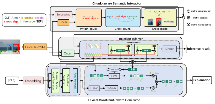
To tackle the two problems, we propose a unified Chunk-aware Alignment and Lexical Constraint based method (CALeC). CALeC contains a Chunk-aware Semantic Interactor (CSI), a relation inferrer and a Lexical Constraint-aware Generator (LeCG). CSI exploits the rich semantics contained in chunks. It adopts a within-chunk interactor and an inter-chunk interactor to learn chunk-level semantics. Then it utilizes a cross-modal interactor to build alignments between chunks and regions, removing the ambiguous alignments. Relation inferrer combines the outputs of CSI and a pre-trained vision-language model to gain a comprehensive representation of the input text-image pair and utilizes an attention-based reasoning network to predict the relation. After that, LeCG generates explanations related to the inference process and input. It utilizes a transformer-based generator to obtain the initial generation probability conditioned on the encoded representation and inferred result. Then LeCG chooses the keywords with higher attention weight during inference as the lexical constraint set and gains a lexical constraint probability over this set. The two probabilities are combined to generate the explanation. Moreover, we utilize a constrained beam sample during testing to score each beam with the probability and number of constraint words occurrences.
We conduct extensive experiments on the current biggest VE-NLE dataset e-SNLI-VE (Kayser et al., 2021). To demonstrate the generalizability of CALeC to other vision-language tasks, we also report results on two VQA-NLE datasets, VQA-X (Park et al., 2018) and VCR (Zellers et al., 2019). Experimental results show that CALeC surpasses the previous state-of-the-art method on a wide range of automatic evaluation metrics. Our quality analysis indicates that the generated explanations of CALeC improve on the aspects of faithfulness and relevance.
In summary, the contributions of our work are three-fold: 1) We propose a unified chunk-aware alignment and lexical constraint based method (CALeC), which contains a chunk-aware semantic interactor (CSI) to exploit the rich semantics of chunks, a relation inferrer to obtain relations, and a lexical constraint-aware generator (LeCG) to produce correlated explanations according to the inference process and input. 2) We introduce CSI and LeCG. CSI explicitly utilizes the chunks and various image regions to build the chunk-aware semantic alignment. LeCG incorporates keywords related to inference results to generate faithful explanations. 3) Experimental results show that CALeC remarkably surpasses existing methods for inference accuracy and explanation faithfulness on the VE-NLE dataset. It also generalizes well across two VQA-NLE datasets.
2. Related Works
To help decrease the class bias and enhance the ability of fine-grained reasoning, Xie et al. (2019) build the visual entailment dataset SNLI-VE, which combines Stanford Natural Language Inference (SNLI) (Bowman et al., 2015) and Flickr30k (Young et al., 2014). They design a two-stream attention network to model the fine-grained cross-modal reasoning and demonstrate their interpretability via attention visualizations. To explain the decision-making process more human-friendly and detailed, Kayser et al. (2021) propose combining visual entailment with natural language explanations and building the first VE-NLE dataset e-SNLI-VE, which is also the current largest NLE dataset for vision-language tasks. Based on it, they establish a benchmark e-ViL for vision-language tasks with NLE, which contains e-SNLI-VE and two VQA-NLE datasets: VQA-X (Park et al., 2018) and VCR (Zellers et al., 2019).
Inference Accuracy. Some works focus on improving inference accuracy. Park et al. (2018) combine multi-modal information via bilinear pooling to predict the answer and utilize an LSTM-based language model to generate the explanation conditioned on the pooling representations. Kayser et al. (2021) propose e-UG that adopts a powerful pre-trained vision-language model UNITER (Chen et al., 2020) to learn joint representations and GPT-2 (Radford et al., 2019) to generate explanations. However, though existing pre-trained models (Chen et al., 2020; Huang et al., 2021; Wang et al., 2021, 2022) have made progress in inference accuracy, the general sequential attentive models focus on building token-level alignment, neglecting the rich semantics contained in phrase.
Explanation Faithfulness. Other works focus on getting more faithful explanations. Wu and Mooney (2019) filter out the samples whose visual explanation does not relevant to the predicted answer via GradCAM (Selvaraju et al., 2017). They utilize an improved Up-Down VQA model (Anderson et al., 2018) for answer inference, and an Up-Down LSTM model (Anderson et al., 2018) to generate explanations. Marasović et al. (2020) use different vision-language models to obtain expressive text-image representations, and feed the encoded representations to GPT-2 (Radford et al., 2019) to generate explanations. However, the language model can only attend to input pairs via attention, treating inference and generation as separate tasks. To enhance the correlation between inference and explanation generation, Patro et al. (2020) use a mutually collaborating module to conduct a jointly adversarial attack on answering and explanation, which also helps improve the robustness of the model. Dua et al. (2021) and Sammani et al. (2022) convert inference as a text generation task and utilize the language model to generate the answer and explanation simultaneously. Nevertheless, they fail to incorporate the critical words of the inference into generation.
3. Methodology
Given an image premise and a text hypothesis , VE-NLE aims to infer the relationship between the input pair and generate an explanation that can reflect the decision-making process. An accurate inference requires a precise understanding of the sentence, and a convincing explanation needs to reflect the inference process faithfully. To this end, we propose CALeC, whose architecture is shown in Figure 2. It consists of three key components: a chunk-aware semantic interactor that exploits the rich semantics contained in phrases (Section 3.1); a relation inferrer that conducts fine-grained inference on the combined outputs of the chunk-aware semantics interactor and a pre-trained vision-language model (Section 3.2); a lexical constraint-aware generator that incorporates the keywords during inference into explanation to improve the faithfulness (Section 3.3). We train CALeC separately and utilize a constrained beam sample during testing. The training and testing detail descriptions are in Section 3.4.
3.1. Chunk-aware Semantic Interactor
We utilize a chunk-aware semantic interactor (CSI) to exploit semantics in phrases and build chunk-level alignment. CSI takes the concatenation of text and image as the input.
For text , we add special tokens [CLS] and [SEP] to denote the start and end of the text. The tokens are fed into an embedding layer to get , where is the representation of -th token. For image with regions, we utilize a pre-trained Faster R-CNN (Ren et al., 2015a) to extract the global image feature and region features. We feed them into a fully-connected layer, obtaining the final representation , where is the representation of the global image and is the representation of the -th region. We use a tagging model to get the borders of text chunks. contains the start index and end index of each chunk, which can be formulated as , and denotes the start index and end token index of -th chunk, respectively. Then, three interactors of different levels are used to learn the chunk-aware representations.
3.1.1. Within-chunk Semantic Interactor
We first adopt a within-chunk semantic interactor to exploit the rich semantics contained in chunks. Each token has access only to the tokens in the same chunk group as itself. For example, as showed in Figure 2, “road” can only attend to “a road sign”. Specifically, for the -th token in the -th chunk, we calculate its attention score to the -th token as follows,
| (1) |
where denotes the representation of -th token, denotes the dimension of the h, and denote the start and end border of -th chunk, respectively. are projection matrices. If and are not in the same chunk, the attention score between them is set to an infinitely negative value so that the resulting attention score after softmax becomes zero.
Then we apply softmax on to obtain the normalized scores , by which we gain the correlation between and other tokens. We aggregate the within-chunk semantics into each token,
| (2) |
where denotes the updated representation of , is the number of tokens, is the projection matrix.
The within-chunk semantic interactor explicitly integrates sentence constituents into , which helps learn the local semantics. To model the relationship between image regions, previous works (Schuster et al., 2015; Liu et al., 2020; Ge et al., 2021) use scene graph parsers to encode regions into visual graphs. We adopt some advanced scene graph parsers approaches (Yang et al., 2018; Zhang et al., 2019) but find the dependencies between regions are ambiguous. These fuzzy relationships can cause error propagation, leading to sub-optimal performance. So we consider each image region as a separate vector, and each region can attend to other regions without limitation. In this way, we integrate the image information into each region representation.
3.1.2. Cross-chunk Semantic Interactor
After obtaining the chunk-level semantics via within-chunk semantic interactor, we utilize a cross-chunk semantic interactor to incorporate the global information into each token. We consider each token as the smallest unit and calculate the attention scores of to the concatenated text-image sequence as follows,
| (3) |
where denotes the representation of the concatenated sequence, are projection matrices.
Then we apply softmax on to obtain the normalized scores , and aggregate the cross-chunk semantics into each token,
| (4) |
where is the projection matrix.
For image representations , we consider each region as the smallest unit and update in a similar way. The cross-chunk semantic interactor helps learn the inter-chunk semantics, fusing the global information in a coarse level.
3.1.3. Cross-modal Semantic Interactor
Cross-modal semantic interactor aims to conduct semantic vision-language fusion in a fine level. Unlike previous works (Park et al., 2018; Chen et al., 2020; Li et al., 2020) that consider each token separately and build vision-language alignments on token-level, we consider each text chunk as a component to build chunk-level alignments. More specifically, we use the average of the tokens in -th chunk as the chunk representation ,
| (5) |
In this way, we aggregate the semantics within the same chunk. Thereafter, we calculate the relative attention of the -th chunk to the -th region,
| (6) |
where denotes the representation of -th region, are projection matrices. measures the correlation between -th chunk and -th region, by which we build chunk-level semantic alignments.
We apply softmax on to obtain the normalized scores , by which we capture the most salient regions related to the -th chunk. We aggregate these regions to each token via ,
| (7) |
where denotes the representation of the -th region, is the number of regions, is projection matrix.
Cross-modal semantic interactor incorporates each chunk and its semantically related regions, which helps remove the ambiguous vision-language alignments and obtain the high-order vision-semantic representations.
3.2. Relation Inferrer
We utilize CSI and a pre-trained vision-language model (i.e., Oscar) to obtain comprehensive joint representations of the input pair. To better retain the alignments of different granularity, we concatenate the outputs of cross-chunk semantic interactor and cross-modal semantic interactor as the final outputs of CSI, represented as , where and denote the text representations and region representations, respectively. Similarly, we denote the outputs of Oscar as .
and contain coarse-grained holistic vision-language representation on token-level and chunk-level, respectively, which ignores the fine-grained alignments of each token. To better incorporate the fine-grained vision-language alignments of different levels, we utilize attention mechanism to look back on and . First, we stack and , and use a linear projection to keep the dimension unchanged,
| (8) |
where is a projection matrix.
Then we concatenate and to obtain a comprehensive representation , which contains token-level and chunk-level cross-modal alignments,
| (9) |
We calculate the relative score between and ,
| (10) |
where are projection matrices, denotes the importance of each alignment. Then we aggregate the salient alignments via and refine ,
| (11) |
where denotes the updated , is projection matrix.
3.3. Lexical Constraint-aware Generator
Lexical constraint-aware generator (LeCG) aims to generate an explanation to interpret the decision-making process. Previous works (Park et al., 2018; Kayser et al., 2021; Sammani et al., 2022) fail to associate explanation generation with the inference process. To alleviate this problem, LeCG explicitly guides explanation generation with the lexical constraint obtained from the inference process.
First, we adopt a transformer-based (Vaswani et al., 2017) language model as the generator. The generator operates cross-attention over the comprehensive representation (obtained via Eq. 9) to exploit the input information. The hidden state of the top layer of the generator at time step is fed to a projection linear and softmax to get the initial generation probability of target token .
Then we construct a word set as the lexical constraint. We add up the attention weights (obtained via Eq. 10) of each attention layer to get the inference attention score of each token, which indicates the importance of each token during inference. We assume the tokens whose score is higher than the median are essential for the decision-making process, and thus they should be in ,
| (13) |
where is the inference attention score of -th token, and is the median score.
We guide the explanation centering around the constraint by combining the initial generation probability with a lexical constraint probability , which is the probability distribution of the tokens within . More specifically, we adopt the cross-attention weights of the generator as the score of each input token. We filter those tokens that are not in and utilize softmax to get the normalized constrained scores,
| (14) |
| (15) |
where denotes the original cross-attention score of at time step from the generator, and denotes the constrained attention scores of each token.
We sum the where as the lexical constraint probability of ,
| (16) |
We use a constrained weight to control the portion of and when calculating the final probability. Following (See et al., 2017; Prabhu and Kann, 2020), we calculate the constrained context vector ,
| (17) |
Then we concatenate with the generator output and the inputs of language model to obtain as follows,
| (18) |
where is a sigmoid activation function, is the learning weight matrix.
Last we obtain the final probability of under lexical constraint:
| (19) |
3.4. Training and Testing
3.4.1. Chunk-aware Semantic Interactor Pre-training
To improve the accuracy of semantic vision-language alignments, we pre-train CSI on the Flickr30k Entities dataset (Plummer et al., 2015). Flickr30k Entities dataset provides the alignments between noun phrases and image regions, where a phrase is aligned to only one region. Note that Flickr30k is also the source corpus of e-SNLI-VE (Kayser et al., 2021), so we split the Flickr30k Entities dataset along e-SNLI-VE to avoid data leakage. During pre-training, we assume that each token should attend to the most semantically relevant region. We sum the attention weights of the cross-modal semantic interactor layers of and apply softmax on it to get the normalized align score . We utilize cross-entropy to enforce the alignment:
| (20) |
where is the align score of -th token to -th region, is the label that indicates whether -th token and -th image origin should be aligned (i.e. 1) or not (i.e. 0), is the number of input tokens and is the number of image regions.
3.4.2. Training Pipeline
The optimization procedure of CALeC contains two stages. First, we train CSI and the relation inferrer for relation inference until the cross-entropy loss converges:
| (21) |
where is the label of the -th relation (e-SNLI-VE) or answer (VQA and VCR), is the probability of the -th relation.
Then we freeze the their parameters and train LeCG for explanation generation. We minimize the negative log-likelihood of LeCG:
| (22) |
where denotes the length of the explanation, denotes the target token at time step .
3.4.3. Testing
To enhance the constraints, we utilize a constrained beam sample during testing. Conventional beam sample (Holtzman et al., 2020) generates a sentence with the highest probability, which ignores the faithfulness of generated explanation. To alleviate this problem, we propose a constrained beam sample that scores each beam with the probability and the number of occurrences of the constraint words. In every step, we multiplied a constraint coefficient to the candidate who generates a word that is in the lexical constraint set . By this way, the candidate who meets more constraints will have a higher score. We choose the candidate with the highest score as the output. The pseudo-code is in Algorithm 1.
4. Experiments
4.1. Settings
4.1.1. Datasets
Following the benchmark e-ViL (Kayser et al., 2021) for vision-language tasks with NLE, we evaluate our method on the VE-NLE dataset e-SNLI-VE (Kayser et al., 2021) and two VQA-NLE datasets VQA-X (Park et al., 2018) and VCR (Zellers et al., 2019). e-SNLI-VE is the current biggest VE-NLE dataset that combines SNLI-VE (Xie et al., 2019) and e-SNLI (Camburu et al., 2018). The training, validation, and test sets contain 401.7k/14.3k/14.7k image-text pairs, respectively. There are three relations of the input pair: entailment, contradiction and neutral. VQA-X is a subset of the VQA v2 dataset (Goyal et al., 2017), in which each sample contains an image, a question, an answer, and the corresponding explanation. The training, validation, and test sets contain 29.5k/1.5k/2k image-text pairs, respectively. VCR provides an image, a question and a list of annotated objects. For each question, a model needs to select one answer from four candidates. After that, it needs to select one explanation from four candidates. The test set for VCR is not publicly available. e-ViL (Kayser et al., 2021) reorganizes the dataset, and reformulates the explanation selection task as a generation task. The training, validation, and test sets contain 191.6k/21.3k/26.5k image-text pairs, respectively.
4.1.2. Evaluation Metrics
Following the e-ViL benchmark, we define three evaluation scores , , and . represents the inference accuracy. represents the average explanation score of examples inferred correctly. This assumes that an explanation is wrong if it justifies an incorrect answer (Kayser et al., 2021). We adopt BLEU-4 (Papineni et al., 2002), ROUGE-L (Lin, 2004), METEOR (Banerjee and Lavie, 2005), CIDEr (Vedantam et al., 2015) and SPICE (Anderson et al., 2016) as the explanation scores. All scores are computed with the publicly available code111https://github.com/tylin/coco-caption. represents the overall performance, which is defined as .
4.1.3. Baselines
Similar to the e-ViL benchmark, we compare our method with five strong baselines. Pointing and Justification (PJ-X) (Park et al., 2018) uses a simplified MCB model (Fukui et al., 2016) as the vision-language encoder and an LSTM-based language model as the decoder. Faithful Multimodal Explanations (FME) (Wu and Mooney, 2019) requires the answer and explanation to focus on the same image regions. It utilizes an improved Up-Down VQA model (Anderson et al., 2018) for answer inference, and an LSTM-based language model for explanation generation. Rationale-VT Transformer (RVT) (Marasović et al., 2020) utilizes different vision-language models to extract vision information and feeds the encoded representations with the question and ground-truth answer to the pre-trained GPT-2 (Radford et al., 2019). Note that RVT omits the question answering part, so we directly quoted the results from the e-ViL benchmark, which extends RVT with Bert (Devlin et al., 2018) to obtain the answer. e-UG (Kayser et al., 2021) combines the powerful pre-trained vision-language model UNITER (Chen et al., 2020) and GPT-2. NLX-GPT (Sammani et al., 2022) utilizes a large-scale pre-trained language model to generate the answer and explanation simultaneously.
4.1.4. Implementation Details
We adopt as the vision-language pre-trained model. We also utilize its parameters to initialize CSI. The number of layers of within-chunk, cross-chunk, and cross-modal semantic interactors are 3/6/3. We use a tagging model (Poth et al., 2021) pre-trained on Chunk-CoNLL2000 (Tjong Kim Sang and Buchholz, 2000) to get the text chunk borders. The number of attention layers of the relation inferrer is 3. We adopt (Radford et al., 2019) as the transformer-based language model in LeCG and randomly initialize the parameters of cross-attention sub-layers. We regard the input text and answer as prefix information and concatenate them before the explanation. For training, we use the Adam optimizer (Kingma and Ba, 2015) with the initial learning rate and linear decay of the learning rate during CSI pre-training and CALeC training pipeline. To maintain the semantic alignment ability of CSI, the initial learning rate of CSI during the training pipeline is set to . The beam size and top-k of beam sample222https://huggingface.co/transformers/internal/generation_utils are set to 5 and 32. The constraint coefficient is set to 0.86.
4.2. Quantitative Analysis
4.2.1. Performance Comparison
| Dataset | Model | B4 | R-L | MET. | CIDEr | SPICE | |||
|---|---|---|---|---|---|---|---|---|---|
| e-SNLI-VE | PJ-X (Park et al., 2018) | 20.40 | 69.20 | 29.48 | 7.30 | 28.60 | 14.70 | 72.50 | 24.30 |
| FME(Wu and Mooney, 2019) | 24.19 | 73.70 | 32.82 | 8.20 | 29.90 | 15.60 | 83.60 | 26.80 | |
| RVT(Marasović et al., 2020) | 24.47 | 72.00 | 33.98 | 9.60 | 27.30 | 18.80 | 81.70 | 32.50 | |
| e-UG∗ (Kayser et al., 2021) | 27.77 | 78.28 | 35.48 | 10.13 | 28.09 | 19.72 | 85.39 | 34.07 | |
| CALeC | 30.28 | 80.92 | 37.42 | 10.53 | 28.53 | 20.02 | 91.61 | 36.42 | |
| \cdashline2-10[1pt/1pt] | NLX-GPT† (Sammani et al., 2022) | 31.07 | 73.91 | 42.04 | 11.90 | 33.40 | 18.10 | 114.70 | 32.10 |
| CALeC† | 37.53 | 80.92 | 46.38 | 13.96 | 35.23 | 19.49 | 127.22 | 35.98 | |
| VQA-X | PJ-X (Park et al., 2018) | 28.76 | 76.40 | 37.64 | 22.70 | 46.00 | 19.70 | 82.70 | 17.10 |
| FME (Wu and Mooney, 2019) | 29.60 | 75.50 | 39.20 | 23.10 | 47.10 | 20.40 | 87.00 | 18.40 | |
| RVT (Marasović et al., 2020) | 20.17 | 68.60 | 29.40 | 17.40 | 42.10 | 19.20 | 52.50 | 15.80 | |
| e-UG (Kayser et al., 2021) | 29.82 | 80.50 | 37.04 | 23.20 | 45.70 | 22.10 | 74.10 | 20.10 | |
| CALeC | 34.43 | 86.38 | 39.85 | 25.47 | 47.02 | 23.38 | 81.58 | 21.82 | |
| \cdashline2-10[1pt/1pt] | NLX-GPT† (Sammani et al., 2022) | 39.18 | 83.07 | 47.16 | 28.50 | 51.50 | 23.10 | 110.60 | 22.10 |
| CALeC† | 40.87 | 86.38 | 47.31 | 29.30 | 51.59 | 23.07 | 110.90 | 21.69 | |
| VCR | PJ-X (Park et al., 2018) | 4.98 | 39.00 | 12.76 | 3.40 | 20.50 | 16.40 | 19.00 | 4.50 |
| FME (Wu and Mooney, 2019) | 9.42 | 48.90 | 19.26 | 4.40 | 22.70 | 17.30 | 27.70 | 24.20 | |
| RVT (Marasović et al., 2020) | 9.29 | 59.00 | 15.74 | 3.80 | 21.90 | 11.20 | 30.10 | 11.70 | |
| e-UG (Kayser et al., 2021) | 11.71 | 69.80 | 16.78 | 4.30 | 22.50 | 11.80 | 32.70 | 12.60 | |
| CALeC | 13.95 | 73.03 | 19.10 | 5.59 | 22.99 | 12.78 | 39.61 | 14.54 | |
| \cdashline2-10[1pt/1pt] | NLX-GPT∗† (Sammani et al., 2022) | 1.88 | 13.45 | 13.96 | 3.16 | 20.76 | 8.62 | 27.72 | 9.54 |
| CALeC† | 15.70 | 73.03 | 21.50 | 6.34 | 25.22 | 12.22 | 49.35 | 14.37 |
We compare our proposed method CALeC against five strong methods on three datasets. The automatic evaluation results are shown in Table 1. We can see that CALeC achieves the best performance, substantially surpassing all the baseline on . By effectively performing chunk-aware semantic alignment and conducting inference over the fine-grained vision-language alignments, CALeC outperforms the strongest baseline model by , , and points on metric across the three datasets, respectively. Though the three datasets focus on different vision-language tasks, CALeC gains accuracy improvement all over them. It suggests that building accurate semantic alignment is a common yet crucial backbone for vision-language models. CALeC also surpasses the state-of-the-art model NLX-GPT on of the three datasets. This verifies that explicitly guiding the generator through lexical constraint can help improve the quality of generated explanations. We observe that of FME in VCR is slightly higher than CALeC. This may be attributed to the lower of FME, so FME only needs to count the more accessible samples when calculating . Note that NLX-GPT does not provide its inference accuracy on the VCR dataset, so we calculate the scores based on their released output results333https://github.com/fawazsammani/nlxgpt. The of NLX-GPT is exceptionally low in VCR. This probably because that the answer of VCR is much longer than the other datasets, so it is harder for NLX-GPT to generate the correct answer.
4.2.2. Ablation Study
| Model | Overall | e-SNLI-VE | VQA-X | VCR |
|---|---|---|---|---|
| CALeC | 31.37 | 37.53 | 40.87 | 15.70 |
| w/o CBS | 30.72↓0.65 | 37.18 | 39.98 | 14.99 |
| w/o LeCG | 30.23↓1.14 | 36.70 | 38.76 | 15.23 |
| w/o LeCG & CBS | 29.68↓1.69 | 35.78 | 38.58 | 14.67 |
| w/o RI & LeCG & CBS | 28.78↓2.59 | 35.29 | 36.58 | 14.48 |
| w/o CSI & RI & LeCG & CBS | 27.48↓3.89 | 34.50 | 33.81 | 14.12 |
We conduct ablation experiments to verify the effectiveness of CSI, relation inferrer, and LeCG in CALeC, which are presented in Table 2. We only list because it summarizes the performance on both and . For a fair comparison, all the evaluated models have the same experimental settings and generate explanations through the beam sample algorithm. The second line verifies the effectiveness of the constrained beam sample. We can see that adding constraints to the conventional beam sample algorithm can help improve the quality of generated explanations. The third line shows the results when we drop LeCG and only retain the transformer-based generator. LeCG has a more significant influence than the constrained beam sample, indicating that directly guiding the generator with constraints can perform better than the post-hoc edit method. When we drop LeCG and the constrained beam sample simultaneously, the decrease in the overall score (1.69) is almost equal to the sum of separate reductions (1.79). This phenomenon shows that these two constrained approaches act at different but complementary points during generation and can jointly improve the quality of explanations. The constraint set is formed based on the relation inferrer and CSI, so they cannot be dropped solely. We drop the relation inferrer along with the constrained methods, in which we directly utilize the linear classifier on the concatenation of the two [CLS] outputs. The scores on the three datasets all decrease, indicating that the relation inferrer can better incorporate the fine-grained alignments of different level. We then drop CSI along with other components, in which the model degenerates into the vanilla transformer-based seq2seq model, i.e., Oscar-GPT. There is a 1.39 net decrease compared to just dropping the relation inferrer, which is higher than other components. This result shows that chunk-aware semantic alignment can greatly benefit vision-language tasks with NLE.
4.3. Qualitative Analysis
4.3.1. Human Evaluation
The automatic NLG metrics do not always reflect the faithfulness of the explanations because explanations can come in different forms and be very generic and data-biased. So we adopt human evaluation to evaluate the faithfulness of explanations. We conduct human evaluation on the test set of e-SNLI-VE, because we do not find the public result of the baseline models on other datasets. Following the e-ViL benchmark, we randomly select 100 test samples with correctly predicted answers. We ask annotators “Given the image and the hypothesis, does the explanation justify the answer?” with four choices: Yes, Weakly yes, Weakly no and No. To ensure the fairness of assessment, the explanations of each sample are shuffled. As shown in the last bar of Figure 3, CALeC gets about 77% positive scores (green region), and about 55% of them are strongly positive (dark green region), which far surpasses other models. The results indicate that our explanations can justify the answer better and reflect the inference process faithfully. We also conduct a human evaluation on CALeC w/o LeCG (the next-to-last bar). The proportion of Yes obviously decreases and the proportion of negative choices increases. This phenomenon verifies that adding constraints on explanation generation can guide the generator to focus on the input and generate explanations faithful to the inference process.

4.3.2. Case Study.
In Figure 4, we show an example with the inference result and explanations of each model on e-SNLI-VE. In this example, CALeC is the only model that infers the correct relation and generates a faithful explanation. In contrast, e-UG mistakes a house for a shop and generates an illogical explanation, and NLX-GPT predicts the wrong answer. In Figure 5, we show some qualitative results from our model on the three datasets. Based on the semantic alignments, the relation inferrer can accurately find the keywords (bold words in input text). LeCG can generate faithful explanations relevant to the inference process and input pair. We observe that although we only provide alignments for noun chunks during pre-training for CSI, it can learn alignments for other part-of-speech chunks (e.g. is giving) during fine-tuning, which may benefit from the cross-chunk semantic interactor.


5. Conclusion and Future Directions
We present a unified Chunk-aware Alignment and Lexical Constraint based method (CALeC) for Visual Entailment with Natural Language Explanations (VE-NLE). Our work is motivated by the need to exploit the rich semantics contained in the chunks and generate explanations faithful to the inference process. This method builds chunk-aware semantic alignment and incorporates the keywords of the inference process into explanation to enhance faithfulness. We conduct extensive experiments on three datasets. Experimental results show that our method achieves state-of-the-art performance on relation inference and explanation generation. It also has strong generalizability over other vision-language tasks. Future work includes building alignments between chunks and visual concepts rather than predetermined regions and improving the relevance between explanations and input image.
Acknowledgements.
This work is jointly supported by grants: Natural Science Foundation of China (No. 62006061 and 61872107), Stable Support Program for Higher Education Institutions of Shenzhen (No. GXWD20201230 155427003-20200824155011001) and Strategic Emerging Industry Development Special Funds of Shenzhen(No. JCYJ20200109113441941).References
- (1)
- Anderson et al. (2016) Peter Anderson, Basura Fernando, Mark Johnson, and Stephen Gould. 2016. Spice: Semantic propositional image caption evaluation. In European conference on computer vision. Springer, 382–398.
- Anderson et al. (2018) Peter Anderson, Xiaodong He, Chris Buehler, Damien Teney, Mark Johnson, Stephen Gould, and Lei Zhang. 2018. Bottom-up and top-down attention for image captioning and visual question answering. In Proceedings of the IEEE conference on computer vision and pattern recognition. 6077–6086.
- Banerjee and Lavie (2005) Satanjeev Banerjee and Alon Lavie. 2005. METEOR: An Automatic Metric for MT Evaluation with Improved Correlation with Human Judgments. In Proceedings of the Workshop on Intrinsic and Extrinsic Evaluation Measures for Machine Translation and/or Summarization@ACL 2005, Ann Arbor, Michigan, USA, June 29, 2005, Jade Goldstein, Alon Lavie, Chin-Yew Lin, and Clare R. Voss (Eds.). Association for Computational Linguistics, 65–72.
- Bowman et al. (2015) Samuel R. Bowman, Gabor Angeli, Christopher Potts, and Christopher D. Manning. 2015. A large annotated corpus for learning natural language inference. In Proceedings of the 2015 Conference on Empirical Methods in Natural Language Processing. Association for Computational Linguistics, Lisbon, Portugal, 632–642.
- Camburu et al. (2018) Oana-Maria Camburu, Tim Rocktäschel, Thomas Lukasiewicz, and Phil Blunsom. 2018. e-snli: Natural language inference with natural language explanations. Advances in Neural Information Processing Systems 31 (2018).
- Chen et al. (2020) Yen-Chun Chen, Linjie Li, Licheng Yu, Ahmed El Kholy, Faisal Ahmed, Zhe Gan, Yu Cheng, and Jingjing Liu. 2020. Uniter: Universal image-text representation learning. In European conference on computer vision. Springer, 104–120.
- Devlin et al. (2018) Jacob Devlin, Ming-Wei Chang, Kenton Lee, and Kristina Toutanova. 2018. Bert: Pre-training of deep bidirectional transformers for language understanding. arXiv preprint arXiv:1810.04805 (2018).
- Dua et al. (2021) Radhika Dua, Sai Srinivas Kancheti, and Vineeth N. Balasubramanian. 2021. Beyond VQA: Generating Multi-Word Answers and Rationales to Visual Questions. In IEEE Conference on Computer Vision and Pattern Recognition Workshops, CVPR Workshops 2021, virtual, June 19-25, 2021. Computer Vision Foundation / IEEE, 1623–1632.
- Fukui et al. (2016) Akira Fukui, Dong Huk Park, Daylen Yang, Anna Rohrbach, Trevor Darrell, and Marcus Rohrbach. 2016. Multimodal Compact Bilinear Pooling for Visual Question Answering and Visual Grounding. In Proceedings of the 2016 Conference on Empirical Methods in Natural Language Processing, EMNLP 2016, Austin, Texas, USA, November 1-4, 2016, Jian Su, Xavier Carreras, and Kevin Duh (Eds.). The Association for Computational Linguistics, 457–468. https://doi.org/10.18653/v1/d16-1044
- Ge et al. (2021) Xuri Ge, Fuhai Chen, Joemon M. Jose, Zhilong Ji, Zhongqin Wu, and Xiao Liu. 2021. Structured Multi-modal Feature Embedding and Alignment for Image-Sentence Retrieval. In MM ’21: ACM Multimedia Conference, Virtual Event, China, October 20 - 24, 2021, Heng Tao Shen, Yueting Zhuang, John R. Smith, Yang Yang, Pablo Cesar, Florian Metze, and Balakrishnan Prabhakaran (Eds.). ACM, 5185–5193.
- Goyal et al. (2017) Yash Goyal, Tejas Khot, Douglas Summers-Stay, Dhruv Batra, and Devi Parikh. 2017. Making the V in VQA Matter: Elevating the Role of Image Understanding in Visual Question Answering. In 2017 IEEE Conference on Computer Vision and Pattern Recognition, CVPR 2017, Honolulu, HI, USA, July 21-26, 2017. IEEE Computer Society, 6325–6334.
- Holtzman et al. (2020) Ari Holtzman, Jan Buys, Li Du, Maxwell Forbes, and Yejin Choi. 2020. The Curious Case of Neural Text Degeneration. In 8th International Conference on Learning Representations, ICLR 2020, Addis Ababa, Ethiopia, April 26-30, 2020.
- Huang et al. (2021) Zhicheng Huang, Zhaoyang Zeng, Yupan Huang, Bei Liu, Dongmei Fu, and Jianlong Fu. 2021. Seeing out of the box: End-to-end pre-training for vision-language representation learning. In Proceedings of the IEEE/CVF Conference on Computer Vision and Pattern Recognition. 12976–12985.
- Kayser et al. (2021) Maxime Kayser, Oana-Maria Camburu, Leonard Salewski, Cornelius Emde, Virginie Do, Zeynep Akata, and Thomas Lukasiewicz. 2021. e-vil: A dataset and benchmark for natural language explanations in vision-language tasks. In Proceedings of the IEEE/CVF International Conference on Computer Vision. 1244–1254.
- Kingma and Ba (2015) Diederik P. Kingma and Jimmy Ba. 2015. Adam: A Method for Stochastic Optimization. In 3rd International Conference on Learning Representations, ICLR 2015, San Diego, CA, USA, May 7-9, 2015, Conference Track Proceedings, Yoshua Bengio and Yann LeCun (Eds.). http://arxiv.org/abs/1412.6980
- Li et al. (2020) Xiujun Li, Xi Yin, Chunyuan Li, Pengchuan Zhang, Xiaowei Hu, Lei Zhang, Lijuan Wang, Houdong Hu, Li Dong, Furu Wei, et al. 2020. Oscar: Object-semantics aligned pre-training for vision-language tasks. In European Conference on Computer Vision. Springer, 121–137.
- Lin (2004) Chin-Yew Lin. 2004. Rouge: A package for automatic evaluation of summaries. In Text summarization branches out. 74–81.
- Lin et al. (2014) Tsung-Yi Lin, Michael Maire, Serge Belongie, James Hays, Pietro Perona, Deva Ramanan, Piotr Dollár, and C Lawrence Zitnick. 2014. Microsoft coco: Common objects in context. In European conference on computer vision. Springer, 740–755.
- Liu et al. (2020) Chunxiao Liu, Zhendong Mao, Tianzhu Zhang, Hongtao Xie, Bin Wang, and Yongdong Zhang. 2020. Graph structured network for image-text matching. In Proceedings of the IEEE/CVF Conference on Computer Vision and Pattern Recognition. 10921–10930.
- Manning et al. (2014) Christopher D. Manning, Mihai Surdeanu, John Bauer, Jenny Rose Finkel, Steven Bethard, and David McClosky. 2014. The Stanford CoreNLP Natural Language Processing Toolkit. In Proceedings of the 52nd Annual Meeting of the Association for Computational Linguistics, ACL 2014, June 22-27, 2014, Baltimore, MD, USA, System Demonstrations. The Association for Computer Linguistics, 55–60. https://doi.org/10.3115/v1/p14-5010
- Marasović et al. (2020) Ana Marasović, Chandra Bhagavatula, Jae sung Park, Ronan Le Bras, Noah A. Smith, and Yejin Choi. 2020. Natural Language Rationales with Full-Stack Visual Reasoning: From Pixels to Semantic Frames to Commonsense Graphs. In Findings of the Association for Computational Linguistics: EMNLP 2020. Association for Computational Linguistics, Online, 2810–2829. https://doi.org/10.18653/v1/2020.findings-emnlp.253
- Papineni et al. (2002) Kishore Papineni, Salim Roukos, Todd Ward, and Wei-Jing Zhu. 2002. Bleu: a Method for Automatic Evaluation of Machine Translation. In Proceedings of the 40th Annual Meeting of the Association for Computational Linguistics, July 6-12, 2002, Philadelphia, PA, USA. ACL, 311–318.
- Park et al. (2018) Dong Huk Park, Lisa Anne Hendricks, Zeynep Akata, Anna Rohrbach, Bernt Schiele, Trevor Darrell, and Marcus Rohrbach. 2018. Multimodal explanations: Justifying decisions and pointing to the evidence. In Proceedings of the IEEE Conference on Computer Vision and Pattern Recognition. 8779–8788.
- Patro et al. (2020) Badri Patro, Shivansh Patel, and Vinay Namboodiri. 2020. Robust Explanations for Visual Question Answering. In Proceedings of the IEEE/CVF Winter Conference on Applications of Computer Vision (WACV).
- Plummer et al. (2015) Bryan A Plummer, Liwei Wang, Chris M Cervantes, Juan C Caicedo, Julia Hockenmaier, and Svetlana Lazebnik. 2015. Flickr30k entities: Collecting region-to-phrase correspondences for richer image-to-sentence models. In Proceedings of the IEEE international conference on computer vision. 2641–2649.
- Poth et al. (2021) Clifton Poth, Jonas Pfeiffer, Andreas Rücklé, and Iryna Gurevych. 2021. What to pre-train on? efficient intermediate task selection. arXiv preprint arXiv:2104.08247 (2021).
- Prabhu and Kann (2020) Nikhil Prabhu and Katharina Kann. 2020. Making a Point: Pointer-Generator Transformers for Disjoint Vocabularies. In Proceedings of the 1st Conference of the Asia-Pacific Chapter of the Association for Computational Linguistics and the 10th International Joint Conference on Natural Language Processing: Student Research Workshop, AACL/IJCNLP 2021, Suzhou, China, December 4-7, 2020. 85–92.
- Radford et al. (2019) Alec Radford, Jeffrey Wu, Rewon Child, David Luan, Dario Amodei, Ilya Sutskever, et al. 2019. Language models are unsupervised multitask learners. OpenAI blog 1, 8 (2019), 9.
- Ren et al. (2015b) Mengye Ren, Ryan Kiros, and Richard Zemel. 2015b. Exploring models and data for image question answering. Advances in neural information processing systems 28 (2015).
- Ren et al. (2015a) Shaoqing Ren, Kaiming He, Ross Girshick, and Jian Sun. 2015a. Faster r-cnn: Towards real-time object detection with region proposal networks. Advances in neural information processing systems 28 (2015).
- Sammani et al. (2022) Fawaz Sammani, Tanmoy Mukherjee, and Nikos Deligiannis. 2022. NLX-GPT: A Model for Natural Language Explanations in Vision and Vision-Language Tasks. CoRR abs/2203.05081 (2022).
- Schuster et al. (2015) Sebastian Schuster, Ranjay Krishna, Angel Chang, Li Fei-Fei, and Christopher D Manning. 2015. Generating semantically precise scene graphs from textual descriptions for improved image retrieval. In Proceedings of the fourth workshop on vision and language. 70–80.
- See et al. (2017) Abigail See, Peter J. Liu, and Christopher D. Manning. 2017. Get To The Point: Summarization with Pointer-Generator Networks. In Proceedings of the 55th Annual Meeting of the Association for Computational Linguistics, ACL 2017, Vancouver, Canada, July 30 - August 4, Volume 1: Long Papers. 1073–1083.
- Selvaraju et al. (2017) Ramprasaath R. Selvaraju, Michael Cogswell, Abhishek Das, Ramakrishna Vedantam, Devi Parikh, and Dhruv Batra. 2017. Grad-CAM: Visual Explanations from Deep Networks via Gradient-Based Localization. In IEEE International Conference on Computer Vision, ICCV 2017, Venice, Italy, October 22-29, 2017. 618–626.
- Tjong Kim Sang and Buchholz (2000) Erik F. Tjong Kim Sang and Sabine Buchholz. 2000. Introduction to the CoNLL-2000 Shared Task Chunking. In Fourth Conference on Computational Natural Language Learning and the Second Learning Language in Logic Workshop.
- Vaswani et al. (2017) Ashish Vaswani, Noam Shazeer, Niki Parmar, Jakob Uszkoreit, Llion Jones, Aidan N Gomez, Łukasz Kaiser, and Illia Polosukhin. 2017. Attention is all you need. Advances in neural information processing systems 30 (2017).
- Vedantam et al. (2015) Ramakrishna Vedantam, C. Lawrence Zitnick, and Devi Parikh. 2015. CIDEr: Consensus-based image description evaluation. In IEEE Conference on Computer Vision and Pattern Recognition, CVPR 2015, Boston, MA, USA, June 7-12, 2015. IEEE Computer Society, 4566–4575.
- Wang et al. (2022) Peng Wang, An Yang, Rui Men, Junyang Lin, Shuai Bai, Zhikang Li, Jianxin Ma, Chang Zhou, Jingren Zhou, and Hongxia Yang. 2022. Unifying Architectures, Tasks, and Modalities Through a Simple Sequence-to-Sequence Learning Framework. CoRR abs/2202.03052 (2022). arXiv:2202.03052
- Wang et al. (2021) Zirui Wang, Jiahui Yu, Adams Wei Yu, Zihang Dai, Yulia Tsvetkov, and Yuan Cao. 2021. Simvlm: Simple visual language model pretraining with weak supervision. arXiv preprint arXiv:2108.10904 (2021).
- Wu and Mooney (2019) Jialin Wu and Raymond J. Mooney. 2019. Faithful Multimodal Explanation for Visual Question Answering. In Proceedings of the 2019 ACL Workshop BlackboxNLP: Analyzing and Interpreting Neural Networks for NLP, BlackboxNLP@ACL 2019, Florence, Italy, August 1, 2019, Tal Linzen, Grzegorz Chrupala, Yonatan Belinkov, and Dieuwke Hupkes (Eds.). Association for Computational Linguistics, 103–112.
- Xie et al. (2019) Ning Xie, Farley Lai, Derek Doran, and Asim Kadav. 2019. Visual Entailment: A Novel Task for Fine-Grained Image Understanding. CoRR abs/1901.06706 (2019).
- Yang et al. (2018) Jianwei Yang, Jiasen Lu, Stefan Lee, Dhruv Batra, and Devi Parikh. 2018. Graph R-CNN for Scene Graph Generation. In Computer Vision - ECCV 2018 - 15th European Conference, Munich, Germany, September 8-14, 2018, Proceedings, Part I (Lecture Notes in Computer Science, Vol. 11205), Vittorio Ferrari, Martial Hebert, Cristian Sminchisescu, and Yair Weiss (Eds.). Springer, 690–706.
- Young et al. (2014) Peter Young, Alice Lai, Micah Hodosh, and Julia Hockenmaier. 2014. From image descriptions to visual denotations: New similarity metrics for semantic inference over event descriptions. Transactions of the Association for Computational Linguistics 2 (2014), 67–78.
- Zellers et al. (2019) Rowan Zellers, Yonatan Bisk, Ali Farhadi, and Yejin Choi. 2019. From recognition to cognition: Visual commonsense reasoning. In Proceedings of the IEEE/CVF conference on computer vision and pattern recognition. 6720–6731.
- Zhang et al. (2019) Ji Zhang, Kevin J Shih, Ahmed Elgammal, Andrew Tao, and Bryan Catanzaro. 2019. Graphical contrastive losses for scene graph parsing. In Proceedings of the IEEE/CVF Conference on Computer Vision and Pattern Recognition. 11535–11543.
- Zhu et al. (2016) Yuke Zhu, Oliver Groth, Michael Bernstein, and Li Fei-Fei. 2016. Visual7w: Grounded question answering in images. In Proceedings of the IEEE conference on computer vision and pattern recognition. 4995–5004.
Appendix A Failure cases
We include failure cases on e-SNLI-VE and VQA-X of our model in Figure 6. We observe that the failure cases mainly involve misinterpretation of image details (orientation between objects, the gender of the people, the breed of the animals, and the characters). These cases show that although CALeC can exploit the rich semantics contained in phrase thorough chunk-aware semantic interactor, it still has limitations on the image comprehension, which can be a future direction of our work. For e-SNLI-VE, we observe that if the relationship is entailment, the model tends to repeat the hypothesis, which may result from the bias of the dataset. Although the answers are predicted wrong, the explanations are faithful to the answers, which shows that the lexical constraint-aware generator can reflect the decision-making process and help correct the model bias.
