Chirality dependence of thermoelectric response in a thermal QCD medium

Introduction- Nuclear matter at a very high temperature and/or baryon density is conceived in terms of deconfined quarks and gluons (dubbed as QGP). Transport coefficients serve as input for modelling the flow of such matter created in relativistic heavy ion collision experiments[1, 2, 3]. These experiments indicate that the created matter is very nearly an ideal fluid with the viscosity being close to the conjectured lower bound[4] arrived at from AdS/CFT correspondence. The QGP may be exposed to magnetic fields ($B$) arising from non-central nucleus-nucleus collisions[5, 6]; its strength depending on the time scale of evolution. A strong $B$ provides the ground for probing the topological properties of QCD vacuum[7, 8], whereas weak $B$ yields some novel phenomenological consequences through the lifting of degeneracy between left and right handed quarks. Our aim is to explore the consequence of this splitting on the thermoelectric response of the medium.

In weak $B$ regime ($m_{0}^{2}\ll eB\ll T^{2}$), the thermoelectric response of the thermal QCD medium assumes a matrix structure :

$$\begin{pmatrix}E_{x}\\ E_{y}\end{pmatrix}=\begin{pmatrix}S&N|\bm{B}|\\ N|\bm{B}|&S\end{pmatrix}\begin{pmatrix}{\nabla T|}_{x}\\ {\nabla T|}_{y}\end{pmatrix}.$$

(1)

The diagonal and nondiagnal elements are Seebeck ($S$) and Nernst ($N|\bm{B}|$) coefficients, respectively, which are the measures of ‘longitudinal’ and ‘transverse’ (analogous to Hall effect) induced electric fields. Large fluctuations in the initial energy density in the heavy-ion collisions[9] translate to significant temperature gradients between the central and peripheral regions of the produced fireball, providing the ideal ground to study thermoelectric phenomena.

We also look at the impact of dimensionality of temperature profile (1-D/2-D) on the Seebeck coefficient. At strong $B$, fermions are constrained to move only in one dimension, i.e. only the lowest Landau level (LLL) is populated. When the strength of $B$ decreases, higher Landau levels start getting occupied, consequently, the constraint on motion of fermions is relaxed and the study of thermoelectric response with a 1-D or 2-D temperature profile becomes plausible. However, the Nernst effect is only manifested in the weak $B$ regime, since the transverse current vanishes at strong $B$.

The $p_{0}=0$, ${\bf{p}}\rightarrow 0$ limit of the denominator of the effective propagator yields the quasiparticle masses as[10, 11]

		$\displaystyle m_{L}^{2}=\frac{L^{2}}{2}\arrowvert_{p_{0}=0,{|\bf{p}|}\rightarrow 0}=m_{th}^{2}+4g^{2}C_{F}M^{2},$		(12)
		$\displaystyle m_{R}^{2}=\frac{R^{2}}{2}|_{p_{0}=0,{|\bf{p}|}\rightarrow 0}=m_{th}^{2}-4g^{2}C_{F}M^{2},$		(13)

thus lifting the degeneracy. Here,

	$\displaystyle M^{2}$	$\displaystyle=\frac{|q_{f}B|}{16\pi^{2}}\left(\frac{\pi T}{2m_{f}}-\text{ln}2+\frac{7\mu^{2}\zeta(3)}{8\pi^{2}T^{2}}\right),$		(14)
	$\displaystyle m_{th}^{2}$	$\displaystyle=\frac{1}{8}g^{2}C_{F}\left(T^{2}+\frac{\mu^{2}}{\pi^{2}}\right).$		(15)

The coupling constant, $g$ is used as in[12]. In the ultra relativistic limit, the chirality of a particle is the same as it’s helicity, so that the right and left chiral modes can be thought of as the up/down spin projections in the direction of momentum ($s_{z}=\pm 1/2$) of the particle, suggesting that the medium generated mass of a collective fermion excitation at very high temperatures ($T\gg m_{0}$) is $s_{z}$ (helicity)-dependent. Such $s_{z}$ dependent quasiparticle masses are already known in condensed matter systems[13, 14].

We use the following Ansatz[17] to solve for $\delta f$ from Eq.(16)

$$f^{L/R}=f_{0}^{L/R}-\tau q\bm{E}\cdot\frac{\partial f_{0}^{L/R}}{\partial\bm{p}}-\bm{\chi}.\frac{\partial f_{0}^{L/R}}{\partial\bm{p}},$$

(18)

where, the effect of $\mathbf{B}$ is encoded in $\bm{\chi}$ ($L/R$ denotes the handedness). We begin with a single flavor system. The components of $\bm{\chi}$, after some algebra, can be expressed conveniently in a matrix form

$$\begin{bmatrix}\chi_{x}\\ \chi_{y}\end{bmatrix}=\begin{bmatrix}\frac{-\omega_{c}\tau^{2}}{1+\omega_{c}^{2}\tau^{2}}q&\frac{\omega_{c}\tau^{2}}{1+\omega_{c}^{2}\tau^{2}}q\\ \frac{-\omega_{c}\tau^{2}}{1+\omega_{c}^{2}\tau^{2}}q&-\frac{\omega_{c}^{2}\tau^{3}}{1+\omega_{c}^{2}\tau^{2}}q\end{bmatrix}\begin{bmatrix}E_{x}\\ E_{y}\end{bmatrix}+\\ \begin{bmatrix}-\frac{\tau}{1+\omega_{c}^{2}\tau^{2}}\left(\frac{\epsilon-\mu}{T}\right)&-\left(\frac{\epsilon-\mu}{T}\right)\frac{\omega_{c}\tau^{2}}{1+\omega_{c}^{2}\tau^{2}}\\ \frac{\omega_{c}\tau^{2}}{1+\omega_{c}^{2}\tau^{2}}\left(\frac{\epsilon-\mu}{T}\right)&-\frac{\tau}{1+\omega_{c}^{2}\tau^{2}}\left(\frac{\epsilon-\mu}{T}\right)\end{bmatrix}\begin{bmatrix}\frac{\partial T}{\partial x}\\[3.60004pt] \frac{\partial T}{\partial y}\end{bmatrix}.$$

The induced 4-current is given by (We drop the $L/R$ notation for brevity):

$$J^{\mu}=qg\int\frac{d^{3}\mbox{p}}{(2\pi)^{3}\epsilon}p^{\mu}\left[\delta f-\overline{\delta f}\right],$$

(19)

where, $\overline{\delta f}$ denotes the contribution from antiparticles. For $\bm{\nabla T}=\frac{\partial T}{\partial x}\bm{\hat{x}}+\frac{\partial T}{\partial y}\bm{\hat{y}}$ the equilibrium condition is $J_{x}=J_{y}=0$, which yields the following equations

	$\displaystyle\left[(C_{1})E_{x}+(C_{2})E_{y}+(C_{3})\frac{\partial T}{\partial x}+(C_{4})\frac{\partial T}{\partial y}\right]=0$
	$\displaystyle\left[-(C_{2})E_{x}+(C_{1})E_{y}-(C_{4})\frac{\partial T}{\partial x}+(C_{3})\frac{\partial T}{\partial y}\right]=0$

Solving for $\bm{E}$ in terms of $\bm{\nabla}T$ leads to the structure

$$\begin{pmatrix}E_{x}\\ E_{y}\end{pmatrix}=\begin{pmatrix}S&N|\bm{B}|\\ -N|\bm{B}|&S\end{pmatrix}\begin{pmatrix}\frac{\partial T}{\partial x}\\[3.60004pt] \frac{\partial T}{\partial y}\end{pmatrix}.$$

(20)

with

	$\displaystyle S$	$\displaystyle=-\frac{C_{1}C_{3}+C_{2}C_{4}}{C_{1}^{2}+C_{2}^{2}},$		(21)
	$\displaystyle N|\bm{B}|$	$\displaystyle=\frac{C_{2}C_{3}-C_{1}C_{4}}{C_{1}^{2}+C_{2}^{2}}.$		(22)

where,

	$\displaystyle C_{1}=q$	$\displaystyle\int\mbox{dp}\,p^{4}\frac{\tau}{\epsilon^{2}(1+\omega_{c}^{2}\tau^{2})}\big{\{}f_{0}(1-f_{0})$
	$\displaystyle+$	$\displaystyle\bar{f_{0}}(1-\bar{f_{0}})\big{\}},$
	$\displaystyle C_{2}=q$	$\displaystyle\int\mbox{dp}\,p^{4}\frac{\omega_{c}\tau^{2}}{\epsilon^{2}(1+\omega_{c}^{2}\tau^{2})}\big{\{}f_{0}(1-f_{0})$
	$\displaystyle-$	$\displaystyle\bar{f_{0}}(1-\bar{f_{0}})\big{\}},$
	$\displaystyle C_{3}=\beta$	$\displaystyle\int\mbox{dp}\,p^{4}\frac{\tau}{\epsilon^{2}(1+\omega_{c}^{2}\tau^{2})}\big{\{}(\epsilon+\mu)\bar{f_{0}}$
		$\displaystyle(1-\bar{f_{0}})-(\epsilon-\mu)f_{0}(1-f_{0})\big{\}},$
	$\displaystyle C_{4}=\beta$	$\displaystyle\int\mbox{dp}\,p^{4}\frac{\omega_{c}\tau^{2}}{\epsilon^{2}(1+\omega_{c}^{2}\tau^{2})}\big{\{}-(\epsilon+\mu)\bar{f_{0}}$
		$\displaystyle(1-\bar{f_{0}})-(\epsilon-\mu)f_{0}(1-f_{0})\big{\}}.$

For the physical medium consisting of $u$ and $d$ quarks, the total currents are given as

	$\displaystyle J_{x}=$	$\displaystyle\sum_{a=u,d}\left[(I_{1})_{a}E_{x}+(I_{2})_{a}E_{y}+(I_{3})_{a}\frac{\partial T}{\partial x}+(I_{4})_{a}\frac{\partial T}{\partial y}\right]$		(23)
	$\displaystyle J_{y}=$	$\displaystyle\sum_{a=u,d}\left[-(I_{2})_{a}E_{x}+(I_{1})_{a}E_{y}-(I_{4})_{a}\frac{\partial T}{\partial x}+(I_{3})_{a}\frac{\partial T}{\partial y}\right].$		(24)

This ultimately leads to

	$\displaystyle S$	$\displaystyle=-\frac{K_{1}K_{3}+K_{2}K_{4}}{K_{1}^{2}+K_{2}^{2}}$		(25)
	$\displaystyle N|\bm{B}|$	$\displaystyle=\frac{K_{2}K_{3}-K_{1}K_{4}}{K_{1}^{2}+K_{2}^{2}},$		(26)

where,

	$\displaystyle K_{1}$	$\displaystyle=\sum_{a=u,d}(I_{1})_{a}\,,\qquad K_{2}=\sum_{a=u,d}(I_{2})_{a}\,,$
	$\displaystyle K_{3}$	$\displaystyle=\sum_{a=u,d}(I_{3})_{a}\,,\qquad\,K_{4}=\sum_{a=u,d}(I_{4})_{a}.$

As mentioned earlier, the Seebeck coefficient can also be evaluated with a 1D temperature profile[18, 19], e.g. $\bm{\nabla}T=\frac{\partial T}{\partial x}\bm{\hat{x}}$. For the composite medium, it is given as

$$S_{1D}=\frac{1}{T}\frac{\sum\limits_{a=u,d}q_{a}(I_{2})_{a}}{\sum\limits_{a=u,d}q_{a}^{2}\,(I_{1})_{a}}=\frac{\sum\limits_{a}S_{a}\,q_{a}^{2}(I_{1})_{a}}{\sum\limits_{a}q_{a}^{2}(I_{1})_{a}},$$

(27)

with

	$\displaystyle I_{1}=q$	$\displaystyle\int\mbox{dp}\,p^{4}\frac{\tau}{\epsilon^{2}(1+\omega_{c}^{2}\tau^{2})}\big{\{}f_{0}(1-f_{0})$
	$\displaystyle+$	$\displaystyle\bar{f_{0}}(1-\bar{f_{0}})\big{\}},$
	$\displaystyle I_{2}=q$	$\displaystyle\int\mbox{dp}\,p^{4}\frac{\tau}{\epsilon^{2}(1+\omega_{c}^{2}\tau^{2})}\big{\{}(\epsilon-\mu)f_{0}(1-f_{0})$
	$\displaystyle-$	$\displaystyle(\epsilon+\mu)\bar{f_{0}}(1-\bar{f_{0}})\big{\}}$

Thus, the total Seebeck coefficient is expressed as a weighted average of the single component coefficients. Such a mathematical structure is absent for the 2D $T$ profile. Since the Nernst coefficient relates the induced electric field and the temperature gradient in mutually transverse directions, it emerges along with the Seebeck coefficient naturally in the 2D setup.

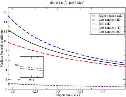
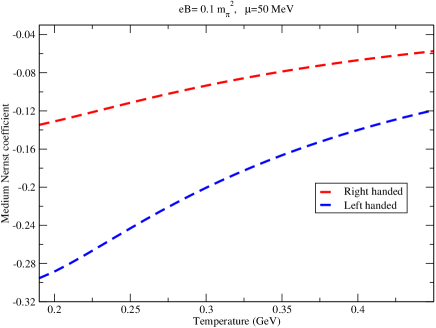
Figures (1) and (2) show the variation of Seebeck and Nernst coefficients of the medium with temperature. It can be seen that the magnitude of the induced electric field in the longitudinal (along $\bm{\nabla T}$) and transverse (perpendicular to $\bm{\nabla T}$) directions shows similar trends as far as variation with temperature is considered; for both the modes, the magnitudes decrease with temperature. Also, for both the coefficients, the $L$ mode elicits a larger comparative response. This can be understood from a numerical perspective. Each of the integrals $C_{1}$, $C_{2}$, $C_{3}$, $C_{4}$ are decreasing functions of the effective mass. However, the extent of decrease follows the hierarchy $\Delta C_{2}>\Delta C_{1}>\Delta C_{4}>\Delta C_{3}$, where $\Delta C$ denotes change in the value of the integral due to a given change in mass. The mathematical expressions of $S$ and $N|\bm{B}|$ then imply that whereas both the numerator and denominator of the expressions decrease with increasing mass, the denominator decreases by a larger amount (because of the presence of $C_{1}$ and $C_{2}$) than the numerator. The value of the fraction, therefore, increases with increasing mass. For comparison, the $B=0$ case is also shown for the Seebeck coefficient. The Nernst coefficient is, however zero for $B=0$, as should be the case.

Fig.(1) shows the impact of the dimension of $T$ profile on the magnitude and temperature behaviour of the Seebeck coefficient. For the 1D setup, Both the $I_{1}$ and $I_{2}$ integrals are decreasing functions of mass, i.e. their values increase in going to the $R$ mode from the $L$ mode. The increase is however greater for $I_{1}$, compared to $I_{2}$ and hence, Eq.(27) dictates the hierarchy that is observed in Fig.(1). As can be seen, there is almost an order magnitude increase in the medium Seebeck coefficient values in the 2-D case. The hierarchy with respect to magnitudes remains the same in the 1-D case with the $L$ mode lying above the $R$ mode for the entire temperature range considered. Compared to the 2-D case, there is stark contrast regarding the extent of splitting (in the Seebeck coefficient magnitude) witnessed in the 1-D setup with a maximum relative difference of 24.5% between the $L$ and $R$ modes (57.1% in the 2-D case). Thus, the magnitude as well as sensitivities to mass and temperature of the thermoelectric response are heightened in the 2-D temperature profile.

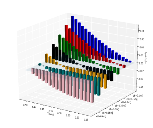
We found that the mass (squared) of the $R$ mode fermion, (Eq.(12)) comes out to be negative for a certain range of combinations of $T$ and $B$ values, which is brought out by Fig.(3). As the magnetic field is increased, the temperature (above $T_{c}\sim 155$ MeV) upto which $m_{R}^{2}$ is negative, also increases. This suggests that the perturbative framework used by us to study the chirality dependence of the thermoelectric response is valid only at regions sufficiently far ($\sim$200 MeV) from the crossover region in the QCD phase diagram for $|eB|>0.2m_{\pi}^{2}$. Another way to look at it is that the condition $eB\ll T^{2}$ is strictly enforced. For $T>T_{c}$, we find from Fig.(3) that $\left|\frac{eB}{T^{2}}\right|_{\text{max}}\sim 0.07$ for $eB=0.1m_{\pi}^{2}$ and $\sim 0.03$ for $eB=0.35m_{\pi}^{2}$. For values of $T$ and $B$ leading to higher values of $\left|\frac{eB}{T^{2}}\right|$, $m_{R}^{2}$ is negative and thus unphysical.

The Seebeck coefficient does not have an explicit $B$ dependence; its $B$ dependence stems from that of the quasiparticle mass. The Nernst coefficient additionally carries an explicit $B$ dependence. As such, its sensitivity to changes in magnetic field strength is comparatively more pronounced. The maximum percentage difference in magnitudes between the $L$ and $R$ modes for the Seebeck and Nernst coefficients is 57.1% and 118.6%, respectively.

References

- Karsch et al. [2008] F. Karsch, D. Kharzeev, and K. Tuchin, Physics Letters B 663, 217 (2008).
- Sasaki and Redlich [2010] C. Sasaki and K. Redlich, Nuclear Physics A 832, 62 (2010).
- S. I. Finazzo and Noronha [2015] H. M. S. I. Finazzo, R. Rougemont and J. Noronha, Journal of High Energy Physics 051, 10.1007/JHEP02(2015)051 (2015).
- Kovtun et al. [2005] P. K. Kovtun, D. T. Son, and A. O. Starinets, Phys. Rev. Lett. 94, 111601 (2005).
- Sokov et al. [2009] V. V. Sokov, A. Y. Illarionov, and V. D. Toneev, International Journal of Modern Physics A 24, 5925 (2009).
- Tuchin [2010] K. Tuchin, Phys. Rev. C 82, 034904 (2010).
- Kharzeev et al. [2008] D. E. Kharzeev, L. D. McLerran, and H. J. Warringa, Nuclear Physics A 803, 227 (2008).
- Fukushima and Hidaka [2018] K. Fukushima and Y. Hidaka, Phys. Rev. Lett. 120, 162301 (2018).
- Schenke et al. [2012] B. Schenke, P. Tribedy, and R. Venugopalan, Phys. Rev. Lett. 108, 252301 (2012).
- Das et al. [2018] A. Das, A. Bandyopadhyay, P. K. Roy, and M. G. Mustafa, Phys. Rev. D 97, 034024 (2018).
- Pushpa and Patra [2022] Pushpa and B. K. Patra, (2022), arXiv:2112.12950 [nucl-th] .
- Ayala et al. [2018] A. Ayala, C. A. Dominguez, S. Hernandez-Ortiz, L. A. Hernandez, M. Loewe, D. M. Paret, and R. Zamora, Phys. Rev. D 98, 031501 (2018).
- Spaek and Gopalan [1990] J. Spaek and P. Gopalan, Phys. Rev. Lett. 64, 2823 (1990).
- Riseborough [2006] P. S. Riseborough, Philosophical Magazine 86, 2581 (2006).
- Hosoya and Kajantie [1985] A. Hosoya and K. Kajantie, Nuclear Physics B 250, 666 (1985).
- Callen [1991] H. B. Callen, Thermodynamics and an Introduction to Thermostatistics, 2nd ed. (Wiley, New York, 1991).
- Feng [2017] B. Feng, Phys. Rev. D 96, 036009 (2017).
- Bhatt et al. [2019] J. R. Bhatt, A. Das, and H. Mishra, Phys. Rev. D 99, 014015 (2019).
- Dey and Patra [2020] D. Dey and B. K. Patra, Phys. Rev. D 102, 096011 (2020).