Chiral phase structure of three flavor QCD
in a background magnetic field

Magnetic fields couple to quarks with their electric charges and through covariant derivative in the continuum,

$\displaystyle D_{\mu}=\partial_{\mu}-igA_{\mu}+iqa_{\mu},$

(1)

where $g$ is the SU(3) gauge coupling and $q$ is the electric charge of a quark. $A_{\mu}$ and $a_{\mu}$ are gauge fields for SU(3) and U(1), respectively. On the lattice the background $U(1)$ magnetic field is introduced by substituting the SU(3) link $U_{\mu}$ by its product with the U(1) link $u_{\mu}$ in the lattice Dirac operator,

$\displaystyle D[U]\to D[uU].$

(2)

In our simulations the magnetic field only points along the $z$-direction. Since the $x$–$y$ plane has boundaries for a finite system size, appropriate boundary conditions need to be imposed. Besides, the magnetic field is realized as a U(1) plaquette, and it introduces non-trivial conditions to the magnitude of the magnetic field as will be depicted next.

Let us denote the lattice size $(N_{x},\;N_{y},\;N_{z},\;N_{t})$ and coordinate as $n_{\mu}=0,\cdots,N_{\mu}-1$ ($\mu=x,\;y,\;z,\;t$). The background magnetic field pointing along the $z$-direction $\vec{B}=(0,0,B)$ is described by the link variable $u_{\mu}(n)$ of the U(1) field, and $u_{\mu}(n)$ is expressed as follows in the Landau gauge Al-Hashimi and Wiese (2009); Bali et al. (2012),

	$\displaystyle u_{x}(n_{x},n_{y},n_{z},n_{t})$	$\displaystyle=\begin{cases}\exp[-iqa^{2}BN_{x}n_{y}]\;\;&(n_{x}=N_{x}-1)\\ 1\;\;&(\text{otherwise})\\ \end{cases}$
	$\displaystyle u_{y}(n_{x},n_{y},n_{z},n_{t})$	$\displaystyle=\exp[iqa^{2}Bn_{x}],$		(3)
	$\displaystyle u_{z}(n_{x},n_{y},n_{z},n_{t})$	$\displaystyle=u_{t}(n_{x},n_{y},n_{z},n_{t})=1.$

The periodic boundary condition for U(1) links is applied for all directions except for the $x$-direction. One-valuedness of the one-particle wave function along with a plaquette requires the following quantization,

$\displaystyle a^{2}qB=\frac{2\pi N_{b}}{N_{x}N_{y}},$

(4)

where $N_{b}\in{\boldsymbol{Z}}$ is the number of magnetic flux through the unit area for the $x$-$y$ plane. The ultraviolet cutoff $a$ also introduces a periodicity of the magnetic field along with $N_{b}$. Namely, a range $0\leq N_{b}<{N_{x}N_{y}}/{4}$, represents an independent magnitude of the magnetic field $B$. In our simulations the 3 mass-degenerate flavors are of up, down and strange quark type, and thus two of the flavors have electrical charge of $q_{d,s}=-\frac{e}{3}$ and the rest one has $q_{u}=\frac{2e}{3}$ with $e$ the electric charge of electron. Thus to satisfy the quantization condition Eq. 4 we take the electric charge $q$ to be that of down quark type, i.e. $q=q_{d,s}=-\frac{e}{3}$. To simplify the notation we use $\hat{b}$ expressed as follows to denote the magnetic field strength

$\displaystyle\hat{b}\equiv a\sqrt{eB}=\sqrt{\frac{6\pi N_{b}}{N_{x}N_{y}}}\,\,.$

(5)

We choose certain values of $N_{b}$ such that $\hat{b}$ are the same in physical units among various lattice sizes which are listed in Table 1.

Based on an earlier estimate of the pion mass in $N_{f}=3$ QCD Karsch et al. (2001) we make a estimate of the scale at the pseudo-critical temperature $T_{pc}^{0}:=T_{pc}(\hat{b}=0)$. We find $m_{\pi}\sim 280$ MeV and $m_{\pi}/T_{pc}^{0}\simeq 1.77$ at $\hat{b}=0$. The values of magnetic field strength for $\hat{b}=1.5$ and 2 thus correspond to $eB/(T_{pc}^{0})^{2}\simeq 36$ and 64, i.e. $eB\sim 11\;m_{\pi}^{2}$ and $eB\sim 20\;m_{\pi}^{2}$, respectively. We further note that the temperature in the explored $\beta$-intervall [5.13,5.19] may change by approximately $25$ MeV, which would lead to corresponding changes in the magnetic field.

Our simulation parameters and statistics are summarized in Tab. 3 - 6. It is worth mentioning that for our largest lattices, i.e. with $N_{\sigma}=24$, we have performed simulations with a hot start (configuration with random elements) and a cold start (configuration with unit elements) to check metastable states around the transition temperature to overcome small tunnelling rates.

An expectation value for an operator ${O}$ for given gauge coupling $\beta$, mass and magnetic flux ${N_{b}}$ is defined by,

$\displaystyle\left\langle O\right\rangle_{\beta,m,N_{b}}$

$\displaystyle=\int\mathcal{D}UP_{\beta,m,N_{b}}[U]\;{O}[U],$

(6)

$\displaystyle P_{\beta,m,N_{b}}[U]$

$\displaystyle=\frac{1}{Z_{\beta,m,N_{b}}}\det\big{[}D_{\text{2/3}}[U,N_{b}]+m\big{]}^{1/4}\det\big{[}D_{\text{-1/3}}[U,N_{b}]+m\big{]}^{2/4}e^{-S_{\text{gauge}}[U;\beta]},$

(7)

where $D$ is the standard staggered Dirac operator and its subscript indicates the electric charge of the related quark. The fractional power, e.g. 1/4 and 2/4, is due to the fourth root of staggered fermions in our simulations.

We measure the chiral condensate for a down type quark ¹¹1 In principle, we can average up, down and strange quark condensate, or up and down. However, we choose down condensate to avoid such arbitrariness.,

$\displaystyle\left\langle\overline{\psi}\psi\right\rangle=\frac{1}{4N_{\sigma}^{3}N_{\tau}}\left\langle\mathrm{Tr}\,\frac{1}{D_{-1/3}+m}\right\rangle,$

(8)

where $\mathrm{Tr}\,[\cdots]$ is a trace over color and space-time, and a factor of $4$ in the denominator adjusts for taste degrees of freedom. Its disconnected susceptibility is given by

$\displaystyle\chi_{\text{disc}}=\frac{1}{16N_{\sigma}^{3}N_{\tau}}\left[\left\langle\left(\mathrm{Tr}\,\frac{1}{D_{-1/3}+m}\right)^{2}\right\rangle-\left\langle\mathrm{Tr}\,\frac{1}{D_{-1/3}+m}\right\rangle^{2}\right].$

(9)

While chiral condensate and its susceptibility are related to chiral symmetry we also compute the Polyakov loop which is related to the deconfinement transition in a pure glue system

$$P=\frac{1}{V}\left\langle\sum_{\vec{x}}\mathrm{Tr}\prod_{t}U_{4}(t,\vec{x})\right\rangle,$$

(10)

and its susceptibility $\chi_{\rm P}$.

We will also analyse the Binder cumulants $B_{M}$ of order parameters $M$, e.g. the chiral condensateBinder (1981) and the Polyakov loop as well as the constructed order parameter from a mixture of the chiral condensate and the gauge action (cf. Eq. 13). $B_{M}$ is defined as follows

$\displaystyle B_{M}(\beta,N_{b})=\frac{\langle(\delta M)^{4}\rangle}{\langle(\delta M)^{2}\rangle^{2}}\;,$

(11)

where $\delta M=M-\langle M\rangle$ gives the deviation of $M$ from its mean value on a given gauge field configuration. From different distributions of $M$ in different phases the value of $B_{M}$ can be obtained and used to distinguish phase transitions. Given that the chiral condensate is the order parameter of the phase transition ²²2The same holds true for other order parameters., for a first order phase transition, $B_{\overline{\psi}\psi}=1$ Ejiri (2008); for a crossover $B_{\overline{\psi}\psi}\simeq 3$ Ejiri (2008); for a second order transition belonging to a Z(2) universality class, $B_{\overline{\psi}\psi}\simeq 1.6$ Blote et al. (1995).

Since our lattice is rather coarse and simulated systems are in the proximity of transitions, we also estimate the effective number of independent configurations $N_{\text{eff}}$ given by

$\displaystyle N_{\text{eff}}=\frac{\#\text{ of trajectories}}{2\tau_{\text{int}}},$

(12)

where $\tau_{\text{int}}$ is the integrated autocorrelation time ³³3 The autocorrelation time and its error are given in Appendix A where $\tau_{\text{int}}$ are rounded in integer for simplicity. for the chiral condensate. Obtained results of $\tau_{\text{int}}$ are listed in Appendix A. Hereafter we will show our results of various quantities in a dimensionless way, i.e. all in units of lattice spacing $a$.

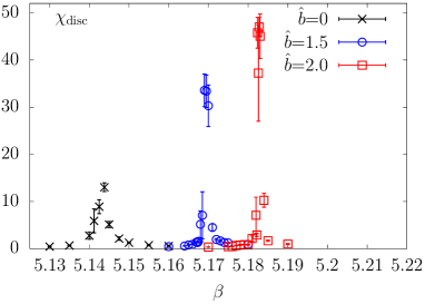
We show the chiral condensate and its disconnected susceptibility for $\hat{b}=0,1.5$ and 2 obtained from lattices with $N_{\sigma}$=16 as a function of the inverse gauge coupling $\beta$ in the left and right plot of Fig. 1, respectively. We recall that the temperature is an increasing function of $\beta$. As seen from the left plot the value of the chiral condensate is enhanced by the magnetic field in the whole temperature region. Namely only the magnetic catalysis is observed. One can also see that the critical $\beta$ value where the chiral condensate drops most rapidly becomes larger as the magnetic field strength increases. This indicates that the transition temperature increases as the magnetic field becomes stronger. Meanwhile as the strength of the magnetic field increases the dropping of chiral condensates becomes more rapidly. This means that the transition becomes stronger with stronger magnetic fields. These two observations are also visible in the behaviour of disconnected chiral susceptibilities as shown in the right plot of Fig. 1. I.e. the peak location of disconnected chiral susceptibility shifts to a larger value of $\beta$ and the peak height of disconnected chiral susceptibility increases as the strength of magnetic field increases.

We show similar plots as Fig. 1 for the Polyakov loop and its susceptibility at $\hat{b}=0,1.5$ and 2 in Fig. 2. The peak location of the Polyakov loop susceptibility as well as the inflection point of the Polyakov loop shifts to larger values of $\beta$, i.e. higher transition temperature with stronger magnetic field. This is similar to the observation from chiral observables. Besides that transition temperatures signalled by the Polyakov loop and its susceptibility are close to those obtained from chiral condensates and disconnected chiral susceptibility. What’s more, it is interesting to see that the peak height of the Polyakov loop susceptibility also becomes higher in a stronger magnetic field, although the Polyakov loop is an order parameter for the confinement-deconfinement phase transition of a pure glue system while the chiral condensate is the order parameter of QCD transitions with vanishing quark massless. This could be due to the fact that neither of these two quantities are the true order parameter but a part of the true order parameter in $N_{f}=3$ QCD⁴⁴4Note that the peak height of Polyakov loop susceptibility also increases as the system approaches the first order phase transition region with smaller values of quark masses for the case of zero magnetic field strength $\hat{b}=0$ Karsch et al. (2001). Karsch et al. (2001); Bazavov et al. (2017).

At vanishing magnetic field the transition is a crossover, and as the magnetic field strength becomes larger the QCD transition becomes stronger. In particular the jumping behavior of the chiral condensate and the Polyakov loop at $\hat{b}$=2 is seen from left plots of Fig. 1 and Fig. 2. This might indicate a first order phase transition. We investigate the nature of the transition by further looking into the time history of chiral condensates. We show in Fig. 3 the time history of chiral condensates near the transition temperature at $\hat{b}=0$ (Top left), $\hat{b}=1.5$ (Top right) and $\hat{b}=2$ (Bottom left) on lattices with $N_{\sigma}=16$. As expected that at vanishing magnetic field ($\hat{b}$=0) there does not exist any metastable behavior, while in the case of $\hat{b}=$1.5 and 2 the metastable behavior becomes obvious. To confirm the metastable behavior seen from the volume of $N_{\sigma}$=16, we also study the case of $\hat{b}=$1.5 with a larger volume, i.e. on $24^{3}\times 4$ lattices. Since in the first order phase transition the tunnelling rate between two metastable states becomes smaller in the larger volume, here we rather investigate on the time history of the chiral condensate obtained from two different kinds of streams, i.e. one starting from a unit configuration (cold) and the other one starting from a random configuration (hot). If there is no first order phase transition chiral condensates obtained from the cold and hot starts will always overlap after thermalization, and if there exist a first order phase transition the two steams from cold and hot starts will stay apart and tunnel from one to the other as the two metastable states in the first order phase transition. The former is observed for the case of $\beta=5.1689$ while the latter is clearly seen for $\beta=5.1698$.

In a short summary, above observations suggest that the transition tends to be a first order for magnetic fields of $\hat{b}\geq$1.5.

In this subsection, we discuss more on the volume dependence of observables at $\hat{b}=0$ and $1.5$ to further confirm the onset of the first order phase transition at $\hat{b}\geq 1.5$. In Fig. 4 we show chiral condensates and their disconnected susceptibilities as a function of $\beta$ obtained from lattices with four different spatial sizes at $\hat{b}=0$ (Top two plots) and $\hat{b}$=1.5 (Bottom two plots). At vanishing magnetic field chiral condensates obtained from $N_{\sigma}=16,$ 20 and 24 are consistent among each other, while large deviations are seen for the results obtained from $N_{\sigma}$=8. In the case of $\hat{b}$=1.5 the finite size effect seems to appear at $\beta$ smaller and close to $\beta_{c}$ starting with a larger volume, i.e. $N_{\sigma}$=16. This could be due to the fact that the system with the presence of a magnetic field tends to have a stronger transition and consequently more statistics is needed to get robust results ⁵⁵5Although we generated two times more configurations at $\hat{b}$=1.5, the effective configurations, however, is two times less than that at $\hat{b}$=0., and that the correlation length in the system becomes longer in the proximity of the true phase transition. Nevertheless, the point where chiral condensates drops most rapidly are consistent among various volumes for both vanishing and nonzero magnetic fields. The is also reflected in the peak locations of disconnected susceptibilities shown in the right column of Fig. 4. In the case of a first order phase transition the disconnected chiral susceptibility should grow linearly in volume. It is more or less the case for disconnected susceptibilities at $\hat{b}$=1.5 as seen from bottom right plot of Fig. 4 and Table 2. And as expected that in the case of vanishing magnetic field the disconnected susceptibility grows slower than linearly in volume as there exists a crossover transition.

We show Binder cumulants of chiral condensates at $\hat{b}=0$ and 1.5 in the left and right plot of Fig. 5, respectively. One can see that at the critical $\beta$ where $\chi_{\rm disc}$ peaks the Binder cumulant reaches to its minimum, which is almost independent of volume at $\hat{b}=0$ and only starts to saturate with $N_{\sigma}\geq$ 20 at $\hat{b}$=1.5. In nonzero magnetic fields the minimum values of Binder cumulant become smaller, i.e. shifting from about 1.6 in the vanishing magnetic field to about 1. This indicates that the transition becomes stronger and tends to become a first order phase transition region at $\hat{b}$=1.5. This is consistent with what we found from chiral condensates and its susceptibilities.

We show similar figures as Fig. 4 and Fig. 5 for Polyakov loops in Fig. 6 and Fig. 7. The observation is similar to that from chiral observables. The volume dependences of Polyakov loops and corresponding susceptibilities are similar to those of chiral observables. Besides, the value for the Binder cumulant has the same tendency. The peak heights of susceptibilities and the minimum values of Binder cumulants for the chiral condensate and the Polyakov loop are summarized in Tab. 2.

In the vicinity of a critical point in 3-flavor QCD, the chiral condensate itself is not a true order parameter, but is part of a mixture of operators that defines the true order parameter $M$ Karsch et al. (2001); Bazavov et al. (2017). In three flavor QCD, such an order parameter can be constructed as a combination of the plaquette action and the chiral condensate as follows Karsch et al. (2001); Bazavov et al. (2017)

$\displaystyle M(\beta,s)={\overline{\psi}\psi}(\beta)+s\,\frac{1}{N_{\sigma}^{3}N_{\tau}}S_{\text{gauge}}(\beta),$

(13)

where $S_{\text{gauge}}=6N_{\sigma}^{3}N_{\tau}\tilde{P}$ and $\tilde{P}$ is the plaquette. Correspondingly, its susceptibility is,

$\displaystyle\chi_{\text{mixed}}=\frac{1}{16N_{\sigma}^{3}N_{\tau}}\left[\left\langle\left(M(\beta,s)\right)^{2}\right\rangle-\left\langle M(\beta,s)\right\rangle^{2}\right].$

(14)

In this work, we do not intend to determine the mixing parameter $s$ and just use the value obtained in the previous work for $a\sqrt{eB}=0$ in Smith and Schmidt (2011), i.e. $s=-0.8$. As will be seen next the results obtained using $s=-0.8$ does not change from $s=0$ qualitatively (cf. Table 2).

We show in the left panel of Fig. 8 the order parameter susceptibility $\chi_{\text{mixed}}$ divided by the spatial volume at $\hat{b}=0$ and 1.5. If the phase transition is of a first order $\chi_{\text{mixed}}$ divided by the spatial volume should be a constant in volume. It is clearly seen that at $\hat{b}$=1.5 data points obtained from lattices with different volumes all overlap at about 0.015 which holds true also towards the infinite volume limit of $(N_{\tau}/N_{\sigma})^{3}\rightarrow 0$, while it is not the case for $\hat{b}=0$. The Binder cumulant of the order parameter is shown in the right panel of Fig. 8. Data points for $\hat{b}=0$ are close the $\mathbb{Z}_{2}$ line, so it seems to belong to a weak second order or crossover transition in the thermodynamic limit. On the other hand, data points for $\hat{b}=1.5$ approach 1 towards the infinite volume limit of $(N_{\tau}/N_{\sigma})^{3}\rightarrow 0$. This is again consistent with the behavior in the first-order phase transition.

In summary, we conclude that the system with $am=0.03$ with magnetic fields $a\sqrt{eB}\geq$1.5 ($eB\gtrsim 11m_{\pi}^{2}$) exists a first order phase transition.

References

- Kharzeev et al. (2013) D. E. Kharzeev, K. Landsteiner, A. Schmitt, and H.-U. Yee, Lect. Notes Phys. 871, 1 (2013), arXiv:1211.6245 [hep-ph] .
- Miransky and Shovkovy (2015) V. A. Miransky and I. A. Shovkovy, Phys. Rept. 576, 1 (2015), arXiv:1503.00732 [hep-ph] .
- D’Elia et al. (2010) M. D’Elia, S. Mukherjee, and F. Sanfilippo, Phys. Rev. D82, 051501 (2010), arXiv:1005.5365 [hep-lat] .
- Bali et al. (2012) G. S. Bali, F. Bruckmann, G. Endrodi, Z. Fodor, S. D. Katz, S. Krieg, A. Schafer, and K. K. Szabo, JHEP 02, 044 (2012), arXiv:1111.4956 [hep-lat] .
- Ilgenfritz et al. (2014) E. M. Ilgenfritz, M. Muller-Preussker, B. Petersson, and A. Schreiber, Phys. Rev. D89, 054512 (2014), arXiv:1310.7876 [hep-lat] .
- Bornyakov et al. (2014) V. G. Bornyakov, P. V. Buividovich, N. Cundy, O. A. Kochetkov, and A. Schäfer, Phys. Rev. D90, 034501 (2014), arXiv:1312.5628 [hep-lat] .
- Bali et al. (2014) G. S. Bali, F. Bruckmann, G. Endrödi, S. D. Katz, and A. Schäfer, JHEP 08, 177 (2014), arXiv:1406.0269 [hep-lat] .
- D’Elia et al. (2018) M. D’Elia, F. Manigrasso, F. Negro, and F. Sanfilippo, Phys. Rev. D98, 054509 (2018), arXiv:1808.07008 [hep-lat] .
- Endrodi et al. (2019) G. Endrodi, M. Giordano, S. D. Katz, T. G. Kovács, and F. Pittler, JHEP 07, 007 (2019), arXiv:1904.10296 [hep-lat] .
- Bonati et al. (2016) C. Bonati, M. D’Elia, M. Mariti, M. Mesiti, F. Negro, A. Rucci, and F. Sanfilippo, Phys. Rev. D94, 094007 (2016), arXiv:1607.08160 [hep-lat] .
- Endrodi (2015) G. Endrodi, JHEP 07, 173 (2015), arXiv:1504.08280 [hep-lat] .
- Cohen and Yamamoto (2014) T. D. Cohen and N. Yamamoto, Phys. Rev. D89, 054029 (2014), arXiv:1310.2234 [hep-ph] .
- Endrodi et al. (2007) G. Endrodi, Z. Fodor, S. D. Katz, and K. K. Szabo, Proceedings, 25th International Symposium on Lattice field theory (Lattice 2007): Regensburg, Germany, July 30-August 4, 2007, PoS LATTICE2007, 182 (2007), arXiv:0710.0998 [hep-lat] .
- Bazavov et al. (2017) A. Bazavov, H. T. Ding, P. Hegde, F. Karsch, E. Laermann, S. Mukherjee, P. Petreczky, and C. Schmidt, Phys. Rev. D95, 074505 (2017), arXiv:1701.03548 [hep-lat] .
- Nakamura et al. (2019) Y. Nakamura, Y. Kuramashi, H. Ohno, and S. Takeda, in 37th International Symposium on Lattice Field Theory (Lattice 2019) Wuhan, Hubei, China, June 16-22, 2019 (2019) arXiv:1909.05441 [hep-lat] .
- Kuramashi et al. (2020) Y. Kuramashi, Y. Nakamura, H. Ohno, and S. Takeda, Phys. Rev. D101, 054509 (2020), arXiv:2001.04398 [hep-lat] .
- Tomiya et al. (2019) A. Tomiya, H.-T. Ding, X.-D. Wang, Y. Zhang, S. Mukherjee, and C. Schmidt, Proceedings, 36th International Symposium on Lattice Field Theory (Lattice 2018): East Lansing, MI, United States, July 22-28, 2018, PoS LATTICE2018, 163 (2019), arXiv:1904.01276 [hep-lat] .
- Tomiya et al. (2018) A. Tomiya, H.-T. Ding, S. Mukherjee, C. Schmidt, and X.-D. Wang, Proceedings, 35th International Symposium on Lattice Field Theory (Lattice 2017): Granada, Spain, June 18-24, 2017, EPJ Web Conf. 175, 07041 (2018), arXiv:1711.02884 [hep-lat] .
- Clark (2006) M. A. Clark, Proceedings, 24th International Symposium on Lattice Field Theory (Lattice 2006): Tucson, USA, July 23-28, 2006, PoS LAT2006, 004 (2006), arXiv:hep-lat/0610048 [hep-lat] .
- Smith and Schmidt (2011) D. Smith and C. Schmidt, Proceedings, 29th International Symposium on Lattice field theory (Lattice 2011): Squaw Valley, Lake Tahoe, USA, July 10-16, 2011, PoS LATTICE2011, 216 (2011), arXiv:1109.6729 [hep-lat] .
- Al-Hashimi and Wiese (2009) M. Al-Hashimi and U.-J. Wiese, Annals Phys. 324, 343 (2009), arXiv:0807.0630 [quant-ph] .
- Binder (1981) K. Binder, Physical Review Letters 47, 693 (1981).
- Ejiri (2008) S. Ejiri, Phys. Rev. D77, 014508 (2008), arXiv:0706.3549 [hep-lat] .
- Blote et al. (1995) H. W. J. Blote, E. Luijten, and J. R. Heringa, J. Phys. A28, 6289 (1995), arXiv:cond-mat/9509016 [cond-mat] .
- Karsch et al. (2001) F. Karsch, E. Laermann, and C. Schmidt, Phys. Lett. B520, 41 (2001), arXiv:hep-lat/0107020 [hep-lat] .
- D’Elia and Negro (2011) M. D’Elia and F. Negro, Physical Review D 83, 114028 (2011).
- Berg and Neuhaus (1992) B. A. Berg and T. Neuhaus, Phys. Rev. Lett. 68, 9 (1992), arXiv:hep-lat/9202004 [hep-lat] .
- Bonati et al. (2018) C. Bonati, M. D’Elia, G. Martinelli, F. Negro, F. Sanfilippo, and A. Todaro, JHEP 11, 170 (2018), arXiv:1807.07954 [hep-lat] .
- Iba (2001) Y. Iba, Int. J. Mod. Phys. C12, 623 (2001), arXiv:cond-mat/0012323 [cond-mat] .
- Wolff (2004) U. Wolff (ALPHA), Comput. Phys. Commun. 156, 143 (2004), [Erratum: Comput. Phys. Commun.176,383(2007)], arXiv:hep-lat/0306017 [hep-lat] .
- Madras and Sokal (1988) N. Madras and A. D. Sokal, J. Statist. Phys. 50, 109 (1988).
- Luscher (2005) M. Luscher, Comput. Phys. Commun. 165, 199 (2005), arXiv:hep-lat/0409106 [hep-lat] .