Chebyshev Inertial Landweber Algorithm
for Linear Inverse Problems

Let $p$ be a real number satisfying $1\leq p<\infty$. The set of infinite sequences $(a_{1},a_{2},\ldots)$ in $\mathbb{F}$ satisfying $\sum_{i=1}^{\infty}|a_{i}|^{p}<\infty$ is denoted by $l^{p}$ where $\mathbb{F}=\mathbb{C}$ or $\mathbb{R}$. If the length of sequences are finite, i.e., a complex or real vector space, we can define a finite dimensional norm space $l^{p}(N)$. The set of measurable functions defined on the closed interval $[a,b]\subset\mathbb{R}$, $\int_{a}^{b}|f(x)|^{p}dx<\infty$ is denoted by $L^{p}(a,b)$.

Let ${\cal H}$ be a complex or real vector space. For any $f,g\in{\cal H}$, an inner product $\langle f,g\rangle$ is assumed to be given. The norm (inner product norm) associated with the inner product is defined by $\|f\|:=\sqrt{\langle f,g\rangle},\quad f\in{\cal H}.$ If the norm space $({\cal H},\|\cdot\|)$ is complete, the space is said to be Hilbert space. The norm spaces $l^{2}$ and $L^{2}(a,b)$ are Hilbert spaces. In the case of $l^{2}$, the inner products are defined by $\langle f,g\rangle:=\left(\sum_{i=1}^{\infty}f_{i}\overline{g_{i}}\right)^{1/2}.$ On the other hand, the inner product for $L^{2}(a,b)$ is defined by $\langle f,g\rangle:=\sqrt{\int_{a}^{b}f(x)\overline{g(x)}dx}.$

Let $T$ be a bounded linear operator on ${\cal H}$. The operator norm of $T$ is defined by $\|T\|:=\sup_{\|f\|=1}\|Tf\|$ where $f$ is an element of ${\cal H}$. For any $x\in{\cal H}$ and an operator $T$, we have the sub-multiplicative inequality

$$\|Tx\|\leq\|T\|\|x\|.$$

(2)

Let $T$ be a linear operator on ${\cal H}$. A complex number $\lambda\in\mathbb{C}$ is an eigenvalue of $T$ if and only if a nonzero vector $x$ in ${\cal H}$ satisfies $Tx=\lambda x$ where $x$ is said to be an eigenvector corresponding to $\lambda$. In the following, the set of all eigenvalues of $T$ is denoted by $\sigma(T)$. The spectral radius of $T$ is given as

$$\rho(T):=\max\{|\lambda|:\lambda\in\sigma(T)\}.$$

(3)

Suppose that $K(x,y)$ satisfies $\int_{a}^{b}\int_{a}^{b}|K(x,y)|dxdy<\infty.$ For any $f\in L^{2}(a,b)$, let $Tf:=\int_{a}^{b}K(x,y)f(y)dy,$ which is a linear operator on $L^{2}(a,b)$ and the operator $T$ is a compact operator [6]. If the kernel function $K(x,y)$ satisfies $K(x,y)=\overline{K(y,x)},$ then the operator $T$ is a compact self-adjoint operator. In the case of the finite dimensional space $l^{2}(N)$, a linear operator defined by a Hermitian matrix $T$ corresponds to a compact self-adjoint operator.

The next theorem plays an important role in our analysis described below.

Let $T$ be a compact self-adjoint operator on ${\cal H}$. It is known that the set of eigenvalues of a compact self-adjoint operator is a countable set of real numbers [6]. Let $\sigma(T):=\{\lambda_{1},\lambda_{2},\ldots\}(\lambda_{i}\in\mathbb{R})$. A polynomial $f(x):=a_{n}x^{n}+a_{n-1}x^{n-1}+\cdots+a_{0}$ defined on $\mathbb{C}$ is analytic over whole $\mathbb{C}$. As a consequence of the spectral mapping theorem, the set of eigenvalues of $f(T)$ is given as $\sigma(f(T))=\{f(\lambda_{1}),f(\lambda_{2}),\ldots\}.$ For a compact self-adjoint operator $T$, we also have

$$\|f(T)\|=\rho(f(T)).$$

(4)

Assume that $x$ is an element in a Hilbert space. The aim of the Landweber iteration is to recover the original signal $x$ from a measurement $y=Tx$ or noisy measurement $y$ where $T$ is a linear operator. The Landweber iteration is a gradient descent algorithm in a Hilbert space to minimize the error functional $(1/2)\|Tx-y\|^{2}.$ The Landweber iteration is defined by the fixed-point iteration

$$x^{(k+1)}=x^{(k)}-\omega T^{*}(Tx^{(k)}-y).$$

(5)

Suppose that we have a fixed-point iteration defined on a Hilbert space ${\cal H}$:

$$x^{(k+1)}=Ax^{(k)}+b,\quad k=0,1,2,\ldots,$$

(6)

where $x^{(k)},b\in{\cal H}$. The operator $A:{\cal H}\rightarrow{\cal H}$ is a compact self-adjoint operator on ${\cal H}$.

Assume also that $A$ is a contraction mapping which has a fixed point $x^{*}\in{\cal H}$ satisfying $x^{*}=Ax^{*}+b,$ where the existence of the fixed point is guaranteed by Banach fixed-point theorem [6]. The inertial iteration [9] corresponding to the original iteration (6) is defined by

$$x^{(k+1)}=x^{(k)}+\omega_{k}\left(Ax^{(k)}+b-x^{(k)}\right),$$

(7)

where $\{\omega_{k}\}$ are called the inertial factors. It should be remarked that the fixed point of the inertial iteration exactly coincides with the fixed point of the original iteration (6).

From the inertial iteration (7), we have the equivalent update equation

$$x^{(k+1)}=(I-\omega_{k}B)x^{(k)}+\omega_{k}b,$$

(8)

where $B:=I-A$. From the assumption that $A$ is a compact self-adjoint operator, we can show $B$ is also compact self-adjoint. Since the fixed point $x^{*}$ satisfies

$$x^{*}=(I-\omega_{k}B)x^{*}+\omega_{k}b,$$

(9)

for any nonnegative $k$ and subtracting (9) from (8), we immediately have a recursive formula on the residual errors:

$$x^{(k+1)}-x^{*}=(I-\omega_{k}B)(x^{(k)}-x^{*}).$$

(10)

In the following discussion, we will assume the following inertial factors satisfying the periodical condition:

$$\omega_{\ell T+j}=\omega_{j},\quad\ell=0,1,2,\ldots,\quad j=0,1,\ldots,T-1,$$

(11)

where a positive integer $T$ represents the period.

Recursively applying (10) multiple times, we can get

$$x^{(T)}-x^{*}=\left(\prod_{k=0}^{T-1}(I-\omega_{k}B)\right)(x^{(0)}-x^{*}).$$

(12)

The norm of the left-hand side can be upper bounded by

	$\displaystyle\|x^{(T)}-x^{*}\|$	$\displaystyle=$	$\displaystyle\left\|\left(\prod_{k=0}^{T-1}(I-\omega_{k}B)\right)(x^{(0)}-x^{*})\right\|$		(13)
		$\displaystyle\leq$	$\displaystyle\left\|\prod_{k=0}^{T-1}(I-\omega_{k}B)\right\|\|x^{(0)}-x^{*}\|$		(14)
		$\displaystyle=$	$\displaystyle\rho\left(\prod_{k=0}^{T-1}(I-\omega_{k}B)\right)\|x^{(0)}-x^{*}\|.$		(15)

The above inequality is based on the sub-multiplicative inequality (2) and the last equality is due to (4).

As we discussed, the operator $B$ is a compact self-adjoint operator and it has countable real eigenvalues, which are denoted by ${\lambda_{k}}(k=1,2,\ldots)$. Hereafter, the minimum and the maximum eigenvalues of $B$ are denoted by $l_{min}$ and $l_{max}$, respectively.

In the following discussion, we will use the inertial factors defined by

$$\omega_{k}^{*}:=\left[\lambda_{+}+\lambda_{-}\cos\left(\frac{2k+1}{2T}\pi\right)\right]^{-1},\ k=0,1,\ldots,T-1,$$

(16)

where $\lambda_{+}:=(l_{max}+l_{min})/2,\quad\lambda_{-}:=(l_{max}-l_{min})/2.$ These inertail factors are called the Chebyshev inertial factors. A Chebyshev inertial factor is the inverse of a root of a Chebyshev polynomial [8, 9].

Let $\beta_{T}(x):=\prod_{k=0}^{T-1}(1-\omega_{k}^{*}x)$. If the Chebyshev inertial factors are employed in the inertial iteration, we can use Lemma 2 proved in [9] to bound $|\beta_{T}(\lambda)|$ as

$$|\beta_{T}(\lambda)|\leq\text{sech}\left(T\cosh^{-1}\left(\frac{\lambda_{+}}{\lambda_{-}}\right)\right).$$

(17)

for $l_{min}\leq\lambda\leq l_{max}$. Combining the spectral mapping theorem and the above inequality, we immediately obtain

$$\rho(\beta_{T}(B))=\rho\left(\prod_{k=0}^{T-1}(I-\omega_{k}B)\right)\leq\text{sech}\left(T\cosh^{-1}\left(\frac{\lambda_{+}}{\lambda_{-}}\right)\right).$$

(18)

The above argument can be summarized in the following theorem.

This theorem implies that the error norm is tightly upper bounded if the iteration index is a multiple of $T$.

Combining the Landweber iteration with the Chebyshev inertial iteration, we have the Chebyshev inertial Landweber algorithm:

	$\displaystyle x^{(k+1)}$	$\displaystyle=$	$\displaystyle x^{(k)}+\omega_{k}^{*}\left(x^{(k)}-\omega T^{*}(Tx^{(k)}-y)-x^{(k)}\right)$		(20)
		$\displaystyle=$	$\displaystyle x^{(k)}-\omega_{k}^{*}\omega T^{*}\left(Tx^{(k)}-y\right).$

The iteration is almost the same as the original Landweber iteration except for the use of the Chebyshev inertial factors $\{\omega_{k}^{*}\}$. It is common to set the inverse of the maximum eigenvalue of $T^{*}T$ to the fixed factor $\omega$.

In this subsection, deconvolution by the Landweber iteration over the Hilbert space ${\cal H}=L^{2}(-\infty,\infty)$ over $\mathbb{R}$ is studied. Suppose that $f,g\in{\cal H}$ are measurable functions on $\mathbb{R}$. The convolution of $f$ and $g$ are defined as

$$y(x):=\int_{-\infty}^{\infty}f(u)g(x-u)du,$$

(21)

which is a compact operator on ${\cal H}$ [6]. We thus can write $y=Gf$ where $G:{\cal H}\rightarrow{\cal H}$ is a compact operator defined by (21) and $f,g\in{\cal H}$. In a context of an inverse problem regarding a linear system involving a convlution, the function $f$ can be considered as a source signal and $g$ represents a point spread function (PSF) or impulse response. In the context of a partial differential equation, $g$ represents the Green’s function or the integral kernel corresponding to a given partial differential equation.

We further assume that $g$ is an even function satisfying $g(x)=g(-x)$. This implies that the operator $G$ is a compact self-adjoint operator. In the following, we try to recover the source signal $f$ from the blurred signal $y$ by using the Landweber iteration on ${\cal H}$ given by $s^{(k+1)}=s^{(k)}-\omega G^{*}(Gs^{(k)}-y),$ where the initial condition is $s^{(0)}:=y.$ Note that $G^{*}=G$ holds due to the assumption on $g$.

In the following experiments shown below, the closed range from $-8.192$ to $8.192$ are discretized into 16384 bins, and convolution integration (21) is approximated by cyclic convolution with 16384-points FFT and frequency domain products. Figure 1 presents the source signal $f$, the convolutional kernel $g$, and the convolved signal $y$.

Figure 2 presents a deconvolution process by the original Landweber algorithm (upper) and the Chebyshev inertial Landweber algorithm (lower). The tentative results $s^{(k)}$ for every 30 iterations are shown. In both cases, we can observe that $s^{(k)}$ gradually approaches to the source signal $f$. This is because $I-\omega G^{*}G$ is a contractive mapping under the setting $\omega=0.3$. Comparing two figures, we can see that the Chebyshev inertial Landweber algorithm shows much faster convergence to the source signal $f$. This observation is also supported by the error curves depicted in Fig.3. The Chebyshev inertial Landweber algorithm $(T=1,2,8)$ shows faster convergence compared with the original Landweber iteration. For example, the error $||s^{(k)}-f||=0.1$ is achieved with $k=100$ with the original Landweber iteration but the Chebyshev iteration requires only $k=25$ iterations.

In this subsection, we will discuss a least square problem closely related to MIMO detection problems. We here assume a finite dimensional Hilbert space ${\cal H}=l^{2}(n)$ on $\mathbb{C}$.

Let $H\in\mathbb{C}^{n\times n}$ be a complex matrix whose elements follow the normal complex Gaussian distribution ${\cal CN}(0,1)$. Our task is to recover a source signal $x\in\mathbb{C}^{n}$ from a noisy linear measurement $y=Hx+w$ where $w$ is a complex Gaussian noise vector. The problem can be seen as a MIMO detection problem where the numbers of transmit and receive antennas are $n$. The least square problem $\hat{x}:=\text{minimize}_{x\in\mathbb{C}^{n}}(1/2)\|y-Hx\|^{2}$ is equivalent to the maximum likelihood estimation rule for the above setting.

In this case, the Landweber iteration is exactly same as a gradient descent process

$$s^{(k+1)}=s^{(k)}-\omega H^{H}(Hs^{(k)}-y)$$

(22)

for minimizing the objective function. It is known that the asymptotic convergence rate is optimal if $\omega=\omega_{opt}:={2}({\lambda_{min}(H^{H}H)+\lambda_{max}(H^{H}H)})^{-1}$ holds. In this case, the matrix $A:=I-\omega_{opt}H^{H}H$ becomes a Hermitian matrix and thus $A$ is a compact self-adjoint operator on ${\cal H}$. This means that we can apply the Chebyshev inertial iteration to the Landweber iteration.

The details of the experiment are summarized as follows. The dimension $n$ is set to $32$. Each element of $x$ is chosen from 8-PSK constellation $\{\exp((2\pi jk)/8)\}(k=0,1,\ldots,7)$ uniformly at random. The optimal factor $\omega_{opt}$ is employed in the Landweber iteration. Each element of the noise vector $w$ follows ${\cal CN}(0,\sigma^{2})$ where $\sigma=10^{-4}$. The minimum and maximum eigenvalues of $\omega_{opt}H^{H}H$ are used as $l_{min}$ and $l_{max}$ for determining the Chebyshev inertial factors.

Figure 4 summarizes the comparison on the squared error norms $\|s^{(k)}-x\|^{2}$ between the original Landweber iteration and the accelerated iterations. From Fig. 4 (left), we can immediately recognize the zigzag-shaped error curves of the Chebyshev inertial Landweber algorithm. This is because the error norm is exponentially upper bounded only when the iteration index $k$ is multiple of $T$ as shown in Theorem 2. It mean that the lower envelope of the zigzag curves can be seen as the guaranteed performance of the Chebyshev inertial Landweber algorithm. Figure 4 (right) indicates the squared errors up to $k=30000$. The proposed schemes (Chebyshev $T=2,8$) shows much faster convergence compared with the original Landweber iteration.

The speed of convergence of the Landweber iteration is dominated by the spectral radius $\rho(A)=\rho\left(I-\omega_{opt}H^{H}H\right).$ On the other hand, $U(T)$ indicates an upper bound of the normalized asymptotic convergence rate depending on the period $T$. Figure 5 (left) presents both $\rho(A)$ and $U(T)$ as functions of $T$. As $T$ becomes larger, the value of $U(T)$ becomes strictly smaller than $\rho(A)$. This means that the Chebyshev inertial iteration certainly accelerates the asymptotic convergence rate. Figure 5 (right) shows approximate error norms derived from $\rho(A)$ and $U(T)$ which are given by $\rho(A)^{k},U(2)^{k},U(8)^{k}$. Although these values does not include the initial errors $\|s_{0}-x\|$, these curves qualitatively explains the behavior of the actual error curves in Fig. 4 (right). These results support the usefulness of the theoretical analysis discussed in the previous section.

It is natural to consider the projected Landweber algorithm [5] for making use of the prior information of the source signal to improve the reconstruction performance. We here examine the detection performance of a simple projected Landweber-based MIMO detection algorithm.

The soft projection operator $\eta:\mathbb{C}\rightarrow\mathbb{C}$ used here is defined by

$$\eta(r):=\frac{\sum_{p\in S}p\exp\left({-|r-p|^{2}}/{\alpha^{2}}\right)}{\sum_{p\in S}\exp\left({-|r-p|^{2}}/{\alpha^{2}}\right)},$$

(23)

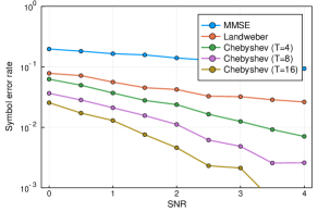
where $S\subset\mathbb{C}$ is a signal constellation [7]. The iteration of the projected Landweber algorithm is fairly simple; the soft projection operator is just element-wisely applied to the output $s^{(k+1)}$ in (22) and then, the output is passed to the inertial iteration process. The details of the experiments are as follows. The channel model is exactly the same as that used in the previous subsection ($32\times 32$ MIMO channel with 8-PSK input). The minimum and maximum eigenvalues $l_{min}$ and $l_{max}$ are determined according to the Marchenko-Pastur law. Figure 6 presents the symbol error rate (SER) of the proposed scheme. The projected Landweber detectors achieves one or two order of magnitude smaller SER than those of the MMSE detector. The accelerated schemes (Chebyshev $T=4,8,16$) provide steeper error curves than that of the projected Landweber detector without Chebyshev inertial iteration (denoted by “Landweber”). This observation supports the potential of the Chebyshev inertial iteration.

References

- [1] L. Landweber, “An iteration formula for Fredholm integral equations of the first kind, ” American journal of mathematics, vol. 73, no. 3, pp. 615–624, 1951.
- [2] F. Vankawala and A. Ganatra, “Modified Landweber algorithm for deblur and denoise Images,” International Journal of Soft Computing and Engineering (IJSCE), vol.5, no.6, pp.79–82, 2016.
- [3] W. Zhang, X. Bao, and J. Dai, “Low-complexity detection based on Landweber method in the uplink of massive MIMO systems,” in Yang et al. Boundary Value Problems, 2017.
- [4] F. Yang, Y.-P. Ren, X.-X. Li and D. G. Li, “Landweber iterative method for identifying a space-dependent source for the time-fractional diffusion equation,” Yang et al. Boundary Value Problems, Springer, 2017.
- [5] P. L. Combettes and J. C. Pesquet, “Proximal splitting methods in signal processing, ” in Fixed-point algorithms for inverse problems in Science and Engineering, Springer-Verlag, pp.185–212, 2011.
- [6] J. Muscat, “Functional analysis,” Springer, 2014.
- [7] S. Takabe, T. Wadayama, Y. C. Eldar, “Complex trainable ISTA for linear and nonlinear inverse problems,” arXiv:1904.07409v2, 2019.
- [8] S. Takabe and T. Wadayama, “Theoretical interpretation of learned step size in deep-unfolded gradient descent, ” arXiv:2001.05142, 2020.
- [9] T. Wadayama and S. Takabe, “Chebyshev inertial iteration for accelerating fixed-point iterations, ” arXiv:2001.03280, 2020.