Chebyshev admissible meshes and Lebesgue constants
of complex polynomial projections
Abstract
We construct admissible polynomial meshes on piecewise polynomial or trigonometric curves of the complex plane, by mapping univariate Chebyshev points. Such meshes can be used for polynomial least-squares, for the extraction of Fekete-like and Leja-like interpolation sets, and also for the evaluation of their Lebesgue constants.
keywords:
admissible polynomial meshes, complex polynomial projections, complex polynomial interpolation, approximate Fekete points, pseudo-Leja sequences, Lebesgue constant.1 Complex Chebyshev-like polynomial meshes
Starting from the seminal paper by Calvi and Levenberg [9], the notion of polynomial (admissible) mesh has been emerging in the last years as a fundamental theoretical and computational tool in polynomial approximation. In the present paper we focus on the univariate complex case. We recall that an admissible polynomial mesh of a polynomially determining compact set (i.e., a polynomial vanishing on vanishes everywhere on ), is a sequence of finite norming subsets such that
| (1) |
where denotes the sup-norm on a continuous or discrete compact set , , , and is a constant independent of . The fact that necessarily holds, since each is -determining. Such a mesh is termed optimal when .
To give only a flavour of the topic, we recall that polynomial meshes are invariant by affine transformations, are stable under small perturbations, and can be assembled by finite union, finite product and algebraic transformations, starting from known instances. Moreover, admissible meshes can be conveniently used for least-square approximation, and contain extremal sets for interpolation of Fekete and Leja type, that can be computed by greedy algorithms; cf., e.g., [1, 4, 9, 18].
Existence of admissible meshes with cardinality has been proved on any connected compact set of whose boundary is a parametric curve with bounded tangent vectors, while optimal admissible meshes are known in special instances; cf. [1]. The following Proposition and Remark show how to construct optimal admissible meshes of Chebyshev type on a wide class of complex curves and domains. To this purpose, we need a basic Lemma.
Lemma 1.
Let , , be an algebraic or trigonometric polynomial with complex coefficients, of degree not exceeding (with in the trigonometric case). Denote by the set of Chebyshev zeros in , , , or the set of Chebyshev extrema in , , .
Consider the points
| (2) |
where
| (3) |
in the algebraic case, and
| (4) |
in the trigonometric case.
Then the following inequality holds for every ,
| (5) |
Proof. In the real algebraic case, (5) is a well-known polynomial inequality originally proved by Ehlich and Zeller [12]. Interestingly, a proof can be given also by the notion of Dubiner distance in , which is tailored to polynomial spaces; cf., e.g., [3, 16]. Indeed, in [20] such a notion has been extended in the subperiodic trigonometric case, i.e. to real trigonometric polynomials on subintervals of the period, namely on with . In such a way, inequality (5) has been proved for real trigonometric polynomials.
We now show how to extend such inequality to algebraic and trigonometric polynomials of a real variable with complex coefficients. Take such that . We can assume that , since (5) trivially holds for . Define the complex number (which lies on the unit circle), and observe that .
Now, consider ; clearly, , and , since is real. Since is a real algebraic or trigonometric polynomial, we can write the chain of inequalities
Proposition 1.
Let be (the image of) a complex parametric curve , , where is an algebraic or trigonometric polynomial of degree (with in the trigonometric case).
Proof. Consider the function composition , which clearly is an algebraic or trigonometric polynomial on with complex coefficients, of degree at most . The result is an immediate consequence of Lemma 1, by observing that
Remark 1.
Let be union of parametric algebraic or trigonometric arcs of degree on , . Then for every , ,
| (7) |
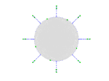
i.e. is an optimal admissible mesh for , by the finite union property of admissible meshes, cf. e.g. [9, Lemma 4]. On the other hand, such is an admissible mesh also for any compact set having outer boundary lying on , with contained in , say , by the maximum modulus principle applied to polynomials (we recall that the outer boundary is the boundary of the unbounded connected component of ). Notice that such a class is very wide: it includes linear polygons, as well as curvilinear polygons with boundary tracked by splines, or by arcs like in polar coordinates with a trigonometric polynomial. See the Figures below for some illustrative examples.
The following Proposition shows that suitable admissible meshes of the form (6) can be conveniently used to evaluate Lebesgue constants, with rigorous error bounds. Again, we begin with a basic Lemma. The result is well-known for interpolation operators (cf. e.g. [19]), nevertheless we prefer to prove it here for more general projection operators (which include for example also least-square approximations). Below by we denote as usual the space of continuous functions on the compact set .
Lemma 2.
Let be a compact set and a linear projection operator such that
| (8) |
where and is a set of generators of . Moreover, let
be the “Lebesgue function” of .
Then the “Lebesgue constant” of , that is its uniform norm, is equal to the sup-norm of the Lebesgue function on
Proof. Inequality is immediate, since
Let such that . Now, the point is to find a continuous function on such that for all such that , and . To this purpose, since let us write , where , and define a function such that . By a deep topological result, the celebrated Tietze extension theorem (cf. e.g. [11, Ch.7, Thm.5.1]), since is trivially continuous on the closed discrete subset , there exists an extension taking values in . Then, is the required function, because and . To prove that , we can clearly restrict to compact domains (the closure of bounded connected open sets). Then we can apply the maximum principle for subharmonic functions to , since each is subharmonic being the modulus of an (entire) holomorphic function and the sum of subharmonic functions is subharmonic; cf. e.g. [15, §7.7].
Remark 2.
Existence of a continuous function as in the proof above can also be proved by Dugundji’s version of Tietze extension theorem, which in its general formulation concerns extension of continuous functions defined on closed subsets of metric spaces and taking values in locally convex topological vector spaces; cf. [11, Ch.9,Thm.6.1]. Applied to the present context, it simply says that defining such that , there exists an extension such that . Thus , because the lie on the unit circle in and hence their convex hull is a polygon lying in the unit disk.
Remark 3.
The structure of projection operators like (8) includes interpolation operators at distinct nodes , where, denoting by , , the Vandermonde-like matrix in any fixed polynomial basis , we have that
| (9) |
are the corresponding fundamental Lagrange polynomials. But also discrete weighted least-squares operators at nodes with positive weights are included. Indeed, denoting by , , the orthonormal polynomials with respect to the corresponding discrete scalar product , we have that
| (10) |
i.e. , where is the reproducing kernel of the discrete scalar product. Notice that in this case (unless where least-squares approximation coincides with interpolation) the are linearly dependent, thus forming a set of generators of .
Proposition 2.
Let the assumptions of Remark 1 be satisfied, and assume that is a linear projection operator as in Lemma 2.
Then the following estimates hold for every ,
| (11) |
and
| (12) |
Proof. Applying inequality (7) to the polynomial , in view of the maximum modulus principle we get
On the other hand and thus , from which we get immediately
Remark 4.
Notice that and thus, if the sampling set is independent of , as . On the other hand, in any case (12) gives the relative error estimate
| (13) |
that is a relative approximation of the Lebesgue constant by . For example, with we already get the Lebesgue constant with a relative error less than , thus correctly estimating its actual order of magnitude that is the relevant parameter in polynomial approximation. On the other hand (11) gives also the rigorous and computable absolute error estimate
| (14) |
2 Numerical tests
In this section we present several numerical tests (implemented in Matlab), concerning the use of complex Chebyshev-like polynomial meshes for interpolation and least-squares approximation, as well as for the evaluation of the corresponding Lebesgue constants. In all these applications we can work on compact sets whose (outer) boundary has the structure described in Remark 1. A preliminary version of the corresponding software along with the demos can be found at [14].
Concerning interpolation, an appealing set is given by the so-called Fekete points, that are points which maximize the modulus of the Vandermonde determinant. As it is well-known, considering their Lebesgue constant it is immediate to get the (over)estimates for the continuum Fekete points (since for each ), and
| (15) |
when they are obtained by extraction from a Chebyshev-like polynomial mesh . However, the continuum Fekete points are explicitly known only in two special instances, the interval (where they are the Gauss-Lobatto points) and the circle (where they are equally spaced in the arclength), in both cases with .
On the other hand, the computation of Fekete points extracted from a polynomial mesh is known to be a NP-hard problem; cf. [10]. Then, we can resort to points that approximately maximize the modulus of the Vandermonde determinant, extracting them from the polynomial mesh by a greedy algorithm. Starting from [7, 18], such approximate Fekete points have been computed by solving the underdetermined system
| (16) |
in a fixed polynomial basis , where is any nonzero vector, by factorization with column pivoting. Indeed, the nonzero components of the solution vector select the interpolation nodes . This procedure corresponds to a greedy determinantal maximization, and the resulting interpolation points asymptotically behave as the continuum Fekete points, in the sense the corresponding uniform discrete probability measure converge weak- to the potential-theoretic equilibrium measure of the compact set; cf. [4, 7] for a full discussion of these aspects, in both the univariate and the multivariate setting.
An interesting alternative is given by Leja points. For a fixed , the points are defined iteratively as , , which means that differently from Fekete points they form a sequence, i.e. the first are Leja points for degree . A relevant result has been recently proved by Totik [19], who showed that the Lebesgue constant of Leja points has subexponential growth (a fact empirically well-known but missing before a theoretical base). On the other hand, it was previously proved in [2] that Leja points behave asymptotically as Fekete points, in the sense the corresponding uniform discrete probability measure converge weak- to the potential-theoretic equilibrium measure of .
The same asymptotic property is shared by the two families of Leja-like sequences that we consider in this paper, namely discrete Leja points and pseudo-Leja points, both corresponding to a greedy discrete maximization on polynomial meshes. Indeed, discrete Leja points can be computed by factorization with row pivoting of the whole matrix in (16), where the pivots select the interpolation points within , a procedure substantially equivalent to compute , ; cf. e.g. [5] for an analysis of this method, also in the multivariate setting. On the other hand, in our implementation we considered the pseudo-Leja points corresponding to the iteration , , after choosing the first point arbitrarily, e.g. is one of the points in with larger imaginary component; cf. [1] (and [13] for a multivariate extension).
In Figures 2 and 4, we plot the Lebesgue constants of interpolation at approximate Fekete, discrete Leja and pseudo-Leja points, extracted from Chebyshev-like polynomial meshes with on six different compact sets (see Figures 1 and 3), for degrees . We also plot the Lebesgue constant of standard least-squares approximation of degree on the whole mesh. All these Lebesgue constants have been computed on the extraction meshes, recalling that with we get a relative error of less than and thus we substantially recover their actual size, cf. (13).
We make some observations on the main computational issues. In order to control the conditioning of the Vandermonde-like matrices, that becomes unacceptable already at moderate degrees with the standard monomial basis, we have chosen to work with a discrete orthonormalization of the shifted and scaled basis , , where is the barycenter of the mesh and . This approach allows to keep well-conditioning up to moderately high polynomial degrees (cf. e.g. [4]). Notice that, in view of (10) with , the Lebesgue constant on the mesh can then be simply computed via the relevant matrices as
| (17) |
where are either the interpolation or the least-squares sampling points, and the factorization of the corresponding Vandermonde-like matrix with (rectangular) hermitian and square upper-triangular, that is .


In the numerical experiments we have considered six complex regions whose (outer) boundaries can be tracked parametrically via one or more algebraic or trigonometric polynomials, in particular:
-
1.
a M-shaped polygon with sides;
-
2.
a curvilinear polygon, with boundary defined parametrically by linear and cubic splines;
-
3.
a sun-shaped domain that consists of a unit disk and 8 rays that are segments of length ;
-
4.
a lune defined as disk difference ;
-
5.
a cardioid, being the closed curve
-
6.
a domain where is the self-intersecting torpedo curve
First we observe that the interpolation points tend to privilege outward angles/tips/cusps as well as convex portions of the boundary and to avoid inward/concave portions, an electrostatic-like behavior that can be interpreted in connection with their potential theoretic background, cf. [17]. We see that the Lebesgue constants of all discrete extremal sets show a slow increase, but those of Leja-like points have a more erratic behavior with larger oscillations and tendentially higher values with respect to approximate Fekete points (a phenomenon already observed in the real multivariate setting, cf. e.g. [6]). On the other hand, Lebesgue constants of least-squares approximation on the whole polynomial mesh have the lowest values with an essentially logarithmic increase, staying below 5 up to degree 50 in all the six examples.
Acknowledgements. Work partially supported by the DOR funds of the University of Padova and by the INdAM-GNCS (A. Sommariva, M. Vianello), and by the National Science Center - Poland, grant Preludium Bis 1, N. 2019/35/O/ST1/02245 (D.J. Kenne). The research cooperation was funded by the program Excellence Initiative – Research University at the Jagiellonian University in Krakòw (A. Sommariva). This research has been accomplished within the RITA “Research ITalian network on Approximation” and the SIMAI Activity Group ANA&A (A. Sommariva, M. Vianello), and the UMI Group TAA “Approximation Theory and Applications” (A. Sommariva).
References
- [1] L. Białas-Cież, J.P. Calvi, Pseudo Leja sequences, Ann. Mat. Pura Appl. 191 (2012), 53–75.
- [2] T. Bloom, L. Bos, C. Christensen, N. Levenberg, Polynomial interpolation of holomorphic functions in and , Rocky Mountain J. Math. 22 (1992), 441–470.
- [3] L. Bos, A Simple Recipe for Modelling a d-cube by Lissajous curves, Dolomites Res. Notes Approx. DRNA 10 (2017), 1–4.
- [4] L. Bos, J.P. Calvi, N. Levenberg, A. Sommariva, M. Vianello, Geometric Weakly Admissible Meshes, Discrete Least Squares Approximations and Approximate Fekete Points, Math. Comp. 80 (2011), 1601–1621.
- [5] L. Bos, S. de Marchi, A. Sommariva, M. Vianello, Computing multivariate Fekete and Leja points by numerical linear algebra, SIAM J. Numer. Anal. 48 (2010), 1984–1999.
- [6] L. Bos, S. de Marchi, A. Sommariva, M. Vianello, On Multivariate Newton Interpolation at Discrete Leja Points, Dolomites Res. Notes Approx. DRNA 4 (2011), 15–20.
- [7] L. Bos, N. Levenberg, On the Approximate Calculation of Fekete Points: the Univariate Case, Electron. Trans. Numer. Anal. 30 (2008), 377–397.
- [8] L. Bos, M. Vianello, Low cardinality admissible meshes on quadrangles, triangles and disks, Math. Inequal. Appl. 15 (2012), 229–235.
- [9] J.P. Calvi, N. Levenberg, Uniform approximation by discrete least squares polynomials, J. Approx. Theory 152 (2008), 82–100.
- [10] A. Civril, M. Magdon-Ismail, On Selecting a Maximum Volume Sub-matrix of a Matrix and Related Problems, Theor. Comput. Sci. 410 (2009), 4801–4811.
- [11] J. Dugundji, Topology, Allyn&Bacon, Boston, 1966.
- [12] H. Ehlich, K. Zeller, Schwankung von Polynomen zwischen Gitter punkten, Math. Z. 86 (1964), 41–-44.
- [13] D.J. Kenne, Multidimensional pseudo-Leja sequences, arXiv:2303.11871.
- [14] D.J. Kenne, A. Sommariva, M. Vianello, CPOLYMESH: Matlab codes for complex polynomial approximation and Lebesgue constants computation by Chebyshev admissible meshes, preliminary version: https://www.math.unipd.it/~alvise/software.html.
- [15] S.G. Krantz, A Guide to Complex Variables, Mathematical Association of America, 2008.
- [16] F. Piazzon, M. Vianello, A note on total degree polynomial optimization by Chebyshev grids, Optim. Lett. 12 (2018), 63–71.
- [17] E.B. Saff, V. Totik, Logarithmic Potentials with External Fields, Springer, 1997.
- [18] A. Sommariva, M. Vianello, Computing approximate Fekete points by QR factorizations of Vandermonde matrices, Comput. Math. Appl. 57 (2009), 1324–1336.
- [19] V. Totik, The Lebesgue constants for Leja points are subexponential, J. Approx. Theory 287 (2023), 105863.
- [20] M. Vianello, Subperiodic Dubiner distance, norming meshes and trigonometric polynomial optimization, Optim. Lett. 12 (2018), 1659–1667.