Charge self-consistent density functional theory plus ghost rotationally-invariant slave-boson theory for correlated materials
Abstract
We present a charge self-consistent density functional theory combined with the ghost-rotationally-invariant slave-boson (DFT+gRISB) formalism for studying correlated materials. This method is applied to SrVO3 and NiO, representing prototypical correlated metals and charge-transfer insulators. For SrVO3, we demonstrate that DFT+gRISB yields an accurate equilibrium volume and effective mass close to experimentally observed values. Regarding NiO, DFT+gRISB enables the simultaneous description of charge transfer and Mott-Hubbard bands, significantly enhancing the accuracy of the original DFT+RISB approach. Furthermore, the calculated equilibrium volume and spectral function reasonably agree with experimental observations.
I Introduction
Simulating strongly correlated materials from first principles remains one of the most formidable challenges in condensed matter physics. The complexities arise from the intricate interplay among electronic charge, spin, and orbital degrees of freedom, as well as the electron’s dual localization and itinerancy character in these materials, driven by strong local Coulomb interactions. This necessitates the use of quantum many-body techniques that go beyond standard ab initio density functional theory (DFT) Hohenberg and Kohn (1964); Kohn and Sham (1965) for their description.
The combination of DFT with dynamical mean field theory (DFT+DMFT) has been extraordinarily successful in addressing this challenge Anisimov et al. (1997a); Lichtenstein et al. (2001). The DMFT, as the first example of a quantum embedding approach, maps the interacting lattice to an auxiliary quantum impurity model with self-consistently determined bath orbitals Georges et al. (1996), allowing an accurate description of the local correlation physics. Moreover, the DFT+DMFT has been extended to charge self-consistency deriving from a functional formulation Kotliar et al. (2006); Held (2007). The method requires a suitable selection of a correlated set of orbitals Savrasov and Kotliar (2004); Pavarini et al. (2004); Pourovskii et al. (2007); Korotin et al. (2008); Haule et al. (2010), the value of the interaction parameters Anisimov et al. (1993); Anisimov et al. (1997b), a suitable double-counting correction Czyżyk and Sawatzky (1994); Anisimov et al. (1997b); Haule (2015), and accurate impurity solvers Gull et al. (2011); Bulla et al. (2008). This framework is now well-developed, and comparisons between experiments and theory have revealed new physics in many correlated materials, shedding light on phenomena such as Mott localization Koga et al. (2004); de’Medici et al. (2005); Yu and Si (2013); Deng et al. (2019), Hund’s physics Georges et al. (2013); de’ Medici (2011); de’ Medici et al. (2011); de’ Medici (2017); Werner et al. (2008); Haule and Kotliar (2009), and the valence fluctuations in correlated systems Savrasov et al. (2006); Shim et al. (2007); Janoschek et al. (2015). Nevertheless, the approach is computationally demanding and sometimes suffers from the so-called sign problem in the Quantum Monte Carlo solver with sizable off-diagonal hybridizations Gull et al. (2011).
Another approach starts from the Gutzwiller approximation (GA) Gutzwiller (1963, 1964); Metzner and Vollhardt (1989); Bünemann et al. (1998); Bünemann and Gebhard (2007); Fabrizio (2007); Lanatà et al. (2008, 2012) and equivalently rotationally-invariant slave-boson (RISB) method Lechermann et al. (2007); Lanatà et al. (2017a), and their combination with DFT Ho et al. (2008); Deng et al. (2008, 2009); Yao et al. (2011a, b); Piefke and Lechermann (2011); Lanatà et al. (2013, 2015, 2015); Lanatà et al. (2017a). These methods, realized as quantum embedding approaches Lanatà et al. (2015); Lanatà (2023), similar to DMFT, map the lattice problem onto an embedded impurity model and are connected to other quantum embedding concepts Knizia and Chan (2012); Lanatà et al. (2015); Ayral et al. (2017); Lee et al. (2019); Lanatà (2023). The RISB framework can capture local Mott, Hund’s, and valence fluctuation physics Yao et al. (2011a); Lanatà et al. (2012, 2013, 2015); Lanatà et al. (2017a), at a lower computational cost compared to DMFT. However, it sometimes suffers from insufficient accuracy, particularly failing to capture the interplay between the Mott physics and charge fluctuations Frank et al. (2021).
The ghost-rotationally-invariant-slave-boson (gRISB) method was recently introduced to overcome these limitations, expanding the RISB variational space by employing auxiliary “ghost” fermionic degrees of freedom Lanatà et al. (2017b); Frank et al. (2021); Lanatà (2022). Studies have shown that gRISB, even with a small number of ghost orbitals, consistently achieves ground-state and spectral properties that closely align with DMFT, across both single- and multi-orbital Hubbard models Lanatà et al. (2017b); Frank et al. (2021); Lee et al. (2023a); Guerci et al. (2019); Mejuto-Zaera and Fabrizio (2023); Lee et al. (2023b). Additionally, numerical evidence indicates that the accuracy of gRISB approaches that of DMFT solutions as the number of ghost bath orbitals is increased Guerci (2019); Lee et al. (2023a); Guerci et al. (2019); Lee et al. (2023b). This accuracy was confirmed through direct comparisons with DMFT, using exact diagonalization as an impurity solver and discretized hybridization functions Caffarel and Krauth (1994). Moreover, the gRISB requires the calculation of only the ground-state single-particle density matrix of the embedding Hamiltonian, avoiding the need to compute dynamic quantities of the impurity model, making it computationally efficient. The gRISB also does not require a bath fitting procedure and can be seamlessly combined with the density matrix renormalization group (DMRG) solvers White (1992, 1993); Schollwöck (2005); Lee et al. (2023b) and machine learning methods Rogers et al. (2021); Frank et al. (2024). These features position gRISB as a promising approach warranting further investigation, particularly in combination with DFT.
In this work, we present a charge self-consistent DFT plus gRISB (DFT+gRISB) formalism to simulate correlated materials. We apply DFT+gRISB to SrVO3 and NiO, representing correlated metal and charge-transfer insulator systems, respectively, and compare the results with DFT+DMFT. For SrVO3, we demonstrate that DFT+gRISB yields reliable total energy and mass renormalization, in good agreement with experiments and DFT+DMFT studies, significantly improving upon the original RISB approach. For NiO, we show that DFT+gRISB provides a consistent description of the charge-transfer insulator, consistent with experimental and DFT+DMFT studies, while DFT+RISB falsely predicts a metallic solution for NiO. The DFT+gRISB total energy is also in good agreement with DFT+DMFT. Finally, we demonstrate the applicability of the DMRG solver within the gRISB framework, allowing for accurate results, including full five d-orbitals.
II Method
In this section, we discuss the formalism of the charge-self-consistent DFT+gRISB approach and the implementation of our DFT+gRISB framework.
II.1 Formalism
The DFT+gRISB functional is encoded in a Lagrange function Lanatà et al. (2015); Kotliar et al. (2006) represented as follows:
| (1) |
where is the total number of electrons in the system, determined by the charge-neutrality condition, is the chemical potential, is the electron density, is the corresponding constraining field, is the Hartree exchange-correlation functional, is the ion-ion energy, is the ionic potential, is the double-counting energy functional associated with the -th impurity Czyżyk and Sawatzky (1994); Anisimov et al. (1997b), is the corresponding occupancy, is the corresponding potential, and and is the corresponding Coulomb interaction and Hund’s coupling interaction, respectively.
The term is the gRISB Lagrange function associated with following many-body Kohn-Sham-Hubbard “reference system,” expressed in second quantization as follows:
| (2) |
where , is the spin variable, is the position variable, indicates both the sum over and the integral over , is the Laplacian, is the Fermionic field operator, is the projector over a generic computational basis span and:
| (3) | ||||
| (4) |
are the annihilation operators associated with the corresponding correlated degrees of freedom, where is the unit cell label, is the momentum, and is the total number of unit cells in the system. The correlated orbital function is denoted by , where encodes both the orbital degrees of freedom and the spin.
The Lagrangian can be formally expressed as follows:
| (5) |
where is the single-particle matrix representation of the so-called quasiparticle Hamiltonian:
| (6) |
for a given computational basis projector and correlated orbital wavefunction , and the local correlated part of the has the form:
| (7) |
with
| (8) |
The matrix elements of and are the so-called renormalization coefficients of the quasiparticle Hamiltonian, is the quasiparticle single-particle density matrix. The and is the uncorrelated and correlated part of the field operator, respectively, defined as follows:
| (9) | ||||
| (10) |
where is the identity operator, , with controlling the accuracy of the gRISB method, and are the so-called quasi-particle annihilation operators. We have also introduced the so-called embedding Hamiltonian of the -th impurity:
| (11) |
The matrix elements of and is the hybridization and bath coupling constants, respectively, is the ground state of , is a Lagrange multiplier enforcing the normalization of , and , are the impurity and bath Fermionic annihilation operators, respectively. The number of spin orbitals in the bath is .
The charge neutrality is enforced by the chemical potential at quasiparticle occupancy , where . The reason for this additional term is to enforce the physical occupancy to be at the total physical valence number , where the quasiparticle occupancy and the physical occupancy differs by a number Frank et al. (2021); Lanatà (2022). The and can also be viewed as the Lagrange multiplier enforcing the gRISB constraints, and is a Lagrange multiplier enforcing the structure of the matrix Lechermann et al. (2007).
The stationary condition of the DFT+gRISB functional leads to the following saddle-point equations:
| (12) | |||
| (13) | |||
| (14) | |||
| (15) | |||
| (16) | |||
| (17) | |||
| (18) | |||
| (19) | |||
| (20) |
where denotes the average over the ground state of , and we introduced the following parameterization of the matrices:
| (21) | ||||
| (22) | ||||
| (23) |
where is an orthonormal basis of the Hermitian matrices Lanatà et al. (2017a). Equation 12 gives rise to the Kohn-Sham potential, and Eq. 14 is the DFT+gRISB charge density, where the local quasiparticle contribution to the density is subtracted and replaced with the contribution from the local physical density matrix Deng et al. (2009). The chemical potential is determined from Eq. 16. The other equations are the standard gRISB equations for model Hamiltonian Lanatà et al. (2017b); Frank et al. (2021); Lanatà (2022); Mejuto-Zaera and Fabrizio (2023); Lee et al. (2023b). The detailed algorithm for solving these equations will be discussed in the next subsection.
With the converged and , one can compute the Green’s function as follows:
| (24) |
where is the vacuum. Equation 24 holds because the is a single-particle Hamiltonian. The spectral function is calculated from , and we use a broadening factor of eV.
The self-energy can be determined from the Dyson equation:
| (25) |
Note that the self-energy is momentum-independent in gRISB, i.e., . The quasiparticle renormalization weight is determined from:
| (26) |
The expectation value of a generic local operator is computed from the embedding wavefunction:
| (27) |
II.2 Implementation
Our implementation closely follows the previous works Lanatà et al. (2015); Lanatà et al. (2017a). We utilize Wien2k for the DFT part of the calculation Blaha et al. (2020). The projector to the correlated orbitals is constructed from the atomic orbital modified from the density functional theory plus embedded dynamical mean-field theory (DFT+eDMFT) code Haule et al. (2010); Yao et al. (2020). The temperature broadening method is utilized for the Brillouin zone integration with a broadening factor of 0.02 eV. The local density approximation functional (LDA) is utilized in our calculation. We use 5000 k-points and 2000 k-points for the NiO and SrVO3, respectively, and the RK is set to 7. The energy window for constructing the low-energy Hubbard model is [-10 eV — 10e V]. The fully localized limit (FFL) is used as our double-counting scheme Czyżyk and Sawatzky (1994); Anisimov et al. (1997b); Haule (2015), where the nominal valence occupancy is set to 8 and 2 for NiO and SrVO3, respectively. We use the DMRG approach implemented in the block2 code to solve the ground-state wavefunction of Zhai et al. (2023). For the DFT+DMFT calculations, we utilize the DFT+eDMFT code with the same parameter setting as in the DFT+gRISB calculations, which provides a consistent benchmark between the DFT+DMFT and DFT+gRISB methods. The continuous-time Quantum Monte Carlo solver is utilized with Monte Carlo steps distributed over 200 CPUs, and the temperature is set to K. For both methods, we treat all five d-orbitals as correlated shells, and the interaction is of full Slater-Condon type Anisimov et al. (1993); Anisimov et al. (1997b).


The DFT+gRISB self-consistent equations are implemented as follows: (1) converge the DFT calculations to obtain the Kohn-Sham eigenvalue and eigenvectors, (2) construct the projector from the Kohn-Sham eigenvector and the local atomic orbitals, (3) solve the gRISB saddle-point equations Eqs. 13-20 with the Kohn-Sham eigenvalues and the projector, (4) use the gRISB saddle-point solution to compute the new charge density from Eq. 14, (4) feedback the new charge density to DFT to update the new exchange-correlated potential (Eq. 12) and go to step (1) until the charge density and total energy is converged. In our calculations, we set the total energy convergence criteria to eV and the charge convergence criteria to .
III Results
III.1 Applications to SrVO3
In this section, we apply DFT+gRISB to SrVO3 and investigate its total energy and electronic structures. This material has been studied extensively in the past decades and serves as an ideal material for benchmarking new approaches Fujimori et al. (1992); Inoue et al. (1995); Yoshimatsu et al. (2010); Liebsch (2003); Pavarini et al. (2004); Sekiyama et al. (2004); Yoshida et al. (2005); Nekrasov et al. (2006); Tomczak et al. (2012); Taranto et al. (2013); Tomczak et al. (2014); Haule et al. (2014); Haule and Birol (2015); Haule (2015); Zhong et al. (2015); Paul and Birol (2019); James et al. (2021); Pickem et al. (2021). It has a cubic perovskite structure, and the main active orbitals around the Fermi level are in the V- shell. The correlation effect is essential in SrVO3, leading to significant renormalization of the bandwidth near the Fermi level.
We first discuss the total energy of the DFT+gRISB. Figure 1 summarized the total energy of LDA, LDA+RISB, LDA+gRISB, and LDA+DMFT as a function of the unit cell volume. First, we reproduce the known fact that LDA underestimates the equilibrium volume at Å, while the experiment observed value is . The LDA+RISB improves the equilibrium volume to towards the experimental value, but the total energy is not consistent with LDA+DMFT at the quantitative level. On the other hand, LDA+gRISB with 15 bath orbitals significantly improves the total energy, in quantitative agreement with the LDA+DMFT results. The equilibrium volume of LDA+gRISB and LDA+DMFT is and , respectively.
We now discuss the electronic structure of SrVO3. Figure 2 are the momentum-resolved spectral function along the high-symmetry points and the orbital resolved density of state calculated from the LDA, LDA+RISB, LDA+gRISB, and LDA+DMFT approaches at the experimental equilibrium volume. The main characters around the Fermi level are the Vanadium’s orbitals. For the LDA calculation, the bandwidth of the bands is around 2 eV. When including the electronic correlation effects at the LDA+RISB level, we observe slight renormalization of the bandwidth by a factor around , which is inconsistent with the LDA+DMFT, where the renormalization factor is around . Moreover, the LDA+RISB electronic structure is almost identical to LDA, implying a weakly correlated metal that is inconsistent with LDA+DMFT. This inconsistency can be remedied by utilizing LDA+gRISB with 15 bath orbitals shown in Fig. 2(c). In the LDA+gRISB results, the bands are renormalized by a factor of in agreement with LDA+DMFT. Moreover, the electronic structure closely resembles LDA+DMFT, except for the upper Hubbard band of the orbitals is approximated by coherent bands in LDA+gRISB, which is an established feature of gRISB Lanatà et al. (2017b); Lee et al. (2023a, b).
The total density of states calculated from LDA+RISB, LDA+gRISB, and LDA+DMFT at the equilibrium volume is shown in Fig. 3, which are compared with the photoemission experiment Sawatzky and Allen (1984). The LDA+gRISB and LDA+DMFT density of states around the Fermi level are in good agreement with each other, while the upper Hubbard band in LDA+gRISB shows a coherent feature. All three methods capture the gap between -2 eV and 0.5 eV and the low energy peaks, mainly attributed to the uncorrelated O and Sr atoms. Finally, we show the orbital-resolved quasiparticle weight and occupancy in Table 1. The LDA+gRISB and LDA+DMFT values are in quantitative agreement. On the other hand, the LDA+RISB captures reliable occupancy, but the quasiparticle weight is overestimated.

| LDA | LDA+RISB | LDA+gRISB | LDA+DMFT | |
|---|---|---|---|---|
| 1 | 0.78 | 0.53 | 0.51 | |
| 1 | 0.89 | 0.75 | 0.78 | |
| 1.68 | 1.56 | 1.53 | 1.51 | |
| 0.80 | 0.64 | 0.66 | 0.66 |
III.2 Applications to NiO
We now apply DFT+gRISB to NiO, which is a prototypical charge-transfer insulator where the Ni- orbitals hybridize with O- to form the so-called Zhang-Rice band between the lower and the upper Hubbard band(Zaanen et al., 1985; Zhang and Rice, 1988; Kuneš et al., 2007a). The DFT+DMFT approach has been applied to NiO and reveals further insight into electronic structure of this charge-transfer insulator as well as its properties with external pressure, doping, and the surface effects (Kuneš et al., 2007a, b; Zhang et al., 2019; Leonov et al., 2016; Mandal et al., 2019a, b; Leonov et al., 2020; Karolak et al., 2010; Zhu et al., 2020). In this work, we focus on the paramagnetic phase of NiO and compare its total energy and electronic structure with the DFT+DMFT results.


The total energy as a function of the unit cell volume is shown in Fig. 4 for LDA, LDA+RISB, LDA+DMFT, and LDA+DMFT. The LDA significantly underestimates the unit cell volume around 16.6 Å and fails to capture the experimentally observed insulating behavior, which is a well-known feature. The LDA+RISB also fails to produce a Mott insulating solution with realistic Coulomb parameters, eV and eV (Anisimov et al., 1991; Kuneš et al., 2007a), utilized in this work. Therefore, its total energy has a large 1 eV discrepancy compared to LDA+DMFT. On the other hand, LDA+gRISB captures the charge transfer insulator behavior, significantly improving the total energy to a quantitative agreement with the LDA+DMFT values, with a difference of around 10 meV. This difference can be attributed to the finite temperature effect K utilized in the LDA+DMFT calculations.
The DFT bandstructure and density of states are shown in Fig. 5(a). Without breaking the spin symmetry, DFT predicts a metallic solution, which is a known problem in DFT for transition metal oxides (Mattheiss, 1972). The bands around the Fermi level contain the O- and Ni- orbital. The Ni-orbitals are located below the Fermi level and are almost completely filled.
Next, we show the DFT+RISB momentum-resolved spectral function and density of states in Fig. 5(b). We utilize the constrained LDA Coulomb parameters eV and eV in our simulations (Anisimov et al., 1991; Kuneš et al., 2007a). In DFT+RISB, the correlation effects only slightly renormalized the bands around the Fermi level with and and the system is far from the metal-insulator transition.
The DFT+gRISB momentum-resolved spectral function and density of states are shown in Fig. 5(c). Here, we use 17 bath orbitals in our DFT+gRISB calculations. The density of states shown in Fig. 5(c) demonstrate that DFT+gRISB accurately captures the charge-transfer insulating behavior in the density of state, where the Hubbard bands are opened in the Ni- orbitals and the Zhang-Rice band is observed around eV with strong - and - hybridization, in good agreement with the DFT+DMFT results shown in Fig. 5(d) and the previous studies (Kuneš et al., 2007a, b; Zhang et al., 2019; Leonov et al., 2016, 2020; Karolak et al., 2010; Zhu et al., 2020). Moreover, the DFT+gRISB momentum-resolved spectral functions captures reliably the dispersive excitations compared to DFT+DMFT, except the incoherent broadening features, which cannot be described within the gRISB framework.
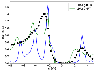
In Fig. 6, we compare the LDA+gRISB total density of states with LDA+DMFT and the photoemission bremsstrahlung-isochromat-spectroscopy (XPS/BIS) (Sawatzky and Allen, 1984). Our LDA+gRISB density of states captures the main features in the XPS/BIS spectrum, where the band gap is about eV, and the heights of the peaks on the band edges are reasonably captured. On the other hand, LDA+DMFT has band gap around 2 eV, smaller than the experimental band gap.
Finally, the orbital-resolved occupancy of different approaches is shown in Table 2. The LDA+gRISB’s occupancy is in good agreement with LDA+DMFT and improves the LDA values. On the other hand, although LDA+RISB fails to capture the charge-transfer insulating solution, its occupancy is identical to the LDA+gRISB values and close to the LDA+DMFT values.
| LDA | LDA+RISB | LDA+gRISB | LDA+DMFT | |
|---|---|---|---|---|
| 2.59 | 2.14 | 2.15 | 2.15 | |
| 5.89 | 5.99 | 5.99 | 5.94 |
IV Conclusions
We present a charge-self-consistent DFT+gRISB approach to correlated materials and demonstrate its performance on two prototypical materials, SrVO3 and NiO, representing the correlated metals and charge transfer insulators. For SrVO3, we show that DFT+gRISB reliably captures the total energy and effective mass compared to the experiment and DFT+DMFT values, significantly improving the original DFT+RISB approach. Furthermore, we show that DFT+gRISB provides a more accurate description of the electronic band structure for strongly correlated materials with a narrow quasiparticle peak and Hubbard bands compared to DFT+RISB. For NiO, DFT+gRISB captures the charge transfer insulating behavior, with the Zhang-Rice band forming between the lower and upper Hubbard bands, significantly improving the DFT+RISB results, which falsely predict a metallic state. The total density of states is in reasonable agreement with the photoemission spectrum. Moreover, our work demonstrates the applicability of DMRG as an impurity solver within the DFT+gRISB framework to reliably simulate correlated full five d-orbital systems.
Future work will extend the DFT+gRISB framework to study the two-particle response functions and interaction vertices (Oelsen et al., 2011; Lee et al., 2021), non-equilibrium dynamics (Schiró and Fabrizio, 2011; Behrmann et al., 2013, 2016; Guerci et al., 2023), and to incorporate gRISB with Wannier-orbital-based projectors and other DFT frameworks and interfaces (Lechermann et al., 2006; Aichhorn et al., 2009, 2011; Parcollet et al., 2015; Aichhorn et al., 2016; Singh et al., 2021; Beck et al., 2022; Grechnev et al., 2007; Di Marco et al., 2009; Grånäs et al., 2012; Shinaoka et al., 2021; Adler et al., 2024; Choi et al., 2019; Kang et al., 2024).
Acknowledgements.
T.-H.L acknowledges discussions with Huanchen Zhai on the block2 DMRG solver. T.-H.L, X.S., and G.K. were supported by the U.S. Department of Energy, Office of Science, Office of Advanced Scientific Computing Research and Office of Basic Energy Sciences, Scientific Discovery through Advanced Computing (SciDAC) program under Award Number DE-SC0022198. C.M. and R.A., was supported by the U.S. Department of Energy, Office of Basic Energy Sciences as part of the Computation Material Science Program. T.-H.L. gratefully acknowledges funding from the Ministry of Science and Technology of Taiwan under Grant No. NSTC 112-2112- M-194-007-MY3. N.L. gratefully acknowledges funding from the Simons Foundation (Grant No. 1030691, N.L.). The part of the work by Y.Y. was supported by the U.S. Department of Energy (DOE), Office of Science, Basic Energy Sciences, Materials Science and Engineering Division, including the grant of computer time at the National Energy Research Scientific Computing Center (NERSC) in Berkeley, California. This part of research was performed at the Ames National Laboratory, which is operated for the U.S. DOE by Iowa State University under Contract No. DE-AC02-07CH11358.References
- Hohenberg and Kohn (1964) P. Hohenberg and W. Kohn, Phys. Rev. 136, B864 (1964), URL https://link.aps.org/doi/10.1103/PhysRev.136.B864.
- Kohn and Sham (1965) W. Kohn and L. J. Sham, Phys. Rev. 140, A1133 (1965), URL https://link.aps.org/doi/10.1103/PhysRev.140.A1133.
- Anisimov et al. (1997a) V. I. Anisimov, A. I. Poteryaev, M. A. Korotin, A. O. Anokhin, and G. Kotliar, Journal of Physics: Condensed Matter 9, 7359 (1997a), URL https://dx.doi.org/10.1088/0953-8984/9/35/010.
- Lichtenstein et al. (2001) A. I. Lichtenstein, M. I. Katsnelson, and G. Kotliar, Phys. Rev. Lett. 87, 067205 (2001), URL https://link.aps.org/doi/10.1103/PhysRevLett.87.067205.
- Georges et al. (1996) A. Georges, G. Kotliar, W. Krauth, and M. J. Rozenberg, Rev. Mod. Phys. 68, 13 (1996), URL https://link.aps.org/doi/10.1103/RevModPhys.68.13.
- Kotliar et al. (2006) G. Kotliar, S. Y. Savrasov, K. Haule, V. S. Oudovenko, O. Parcollet, and C. A. Marianetti, Rev. Mod. Phys. 78, 865 (2006), URL https://link.aps.org/doi/10.1103/RevModPhys.78.865.
- Held (2007) K. Held, Advances in Physics 56, 829 (2007), eprint https://doi.org/10.1080/00018730701619647, URL https://doi.org/10.1080/00018730701619647.
- Savrasov and Kotliar (2004) S. Y. Savrasov and G. Kotliar, Phys. Rev. B 69, 245101 (2004), URL https://link.aps.org/doi/10.1103/PhysRevB.69.245101.
- Pavarini et al. (2004) E. Pavarini, S. Biermann, A. Poteryaev, A. I. Lichtenstein, A. Georges, and O. K. Andersen, Phys. Rev. Lett. 92, 176403 (2004), URL https://link.aps.org/doi/10.1103/PhysRevLett.92.176403.
- Pourovskii et al. (2007) L. V. Pourovskii, B. Amadon, S. Biermann, and A. Georges, Phys. Rev. B 76, 235101 (2007), URL https://link.aps.org/doi/10.1103/PhysRevB.76.235101.
- Korotin et al. (2008) D. Korotin, A. V. Kozhevnikov, S. L. Skornyakov, I. Leonov, N. Binggeli, V. I. Anisimov, and G. Trimarchi, The European Physical Journal B 65, 91 (2008), URL https://doi.org/10.1140/epjb/e2008-00326-3.
- Haule et al. (2010) K. Haule, C.-H. Yee, and K. Kim, Phys. Rev. B 81, 195107 (2010), URL https://link.aps.org/doi/10.1103/PhysRevB.81.195107.
- Anisimov et al. (1993) V. I. Anisimov, I. V. Solovyev, M. A. Korotin, M. T. Czyżyk, and G. A. Sawatzky, Phys. Rev. B 48, 16929 (1993), URL https://link.aps.org/doi/10.1103/PhysRevB.48.16929.
- Anisimov et al. (1997b) V. I. Anisimov, F. Aryasetiawan, and A. I. Lichtenstein, Journal of Physics: Condensed Matter 9, 767 (1997b), URL https://dx.doi.org/10.1088/0953-8984/9/4/002.
- Czyżyk and Sawatzky (1994) M. T. Czyżyk and G. A. Sawatzky, Phys. Rev. B 49, 14211 (1994), URL https://link.aps.org/doi/10.1103/PhysRevB.49.14211.
- Haule (2015) K. Haule, Phys. Rev. Lett. 115, 196403 (2015), URL https://link.aps.org/doi/10.1103/PhysRevLett.115.196403.
- Gull et al. (2011) E. Gull, A. J. Millis, A. I. Lichtenstein, A. N. Rubtsov, M. Troyer, and P. Werner, Rev. Mod. Phys. 83, 349 (2011), URL https://link.aps.org/doi/10.1103/RevModPhys.83.349.
- Bulla et al. (2008) R. Bulla, T. A. Costi, and T. Pruschke, Rev. Mod. Phys. 80, 395 (2008), URL https://link.aps.org/doi/10.1103/RevModPhys.80.395.
- Koga et al. (2004) A. Koga, N. Kawakami, T. M. Rice, and M. Sigrist, Phys. Rev. Lett. 92, 216402 (2004), URL https://link.aps.org/doi/10.1103/PhysRevLett.92.216402.
- de’Medici et al. (2005) L. de’Medici, A. Georges, and S. Biermann, Phys. Rev. B 72, 205124 (2005), URL https://link.aps.org/doi/10.1103/PhysRevB.72.205124.
- Yu and Si (2013) R. Yu and Q. Si, Phys. Rev. Lett. 110, 146402 (2013), URL https://link.aps.org/doi/10.1103/PhysRevLett.110.146402.
- Deng et al. (2019) X. Deng, K. M. Stadler, K. Haule, A. Weichselbaum, J. von Delft, and G. Kotliar, Nature Communications 10, 2721 (2019), ISSN 2041-1723, URL https://doi.org/10.1038/s41467-019-10257-2.
- Georges et al. (2013) A. Georges, L. de’ Medici, and J. Mravlje, Annual Review of Condensed Matter Physics 4, 137 (2013), URL https://doi.org/10.1146/annurev-conmatphys-020911-125045.
- de’ Medici (2011) L. de’ Medici, Phys. Rev. B 83, 205112 (2011), URL https://link.aps.org/doi/10.1103/PhysRevB.83.205112.
- de’ Medici et al. (2011) L. de’ Medici, J. Mravlje, and A. Georges, Phys. Rev. Lett. 107, 256401 (2011), URL https://link.aps.org/doi/10.1103/PhysRevLett.107.256401.
- de’ Medici (2017) L. de’ Medici, Phys. Rev. Lett. 118, 167003 (2017), URL https://link.aps.org/doi/10.1103/PhysRevLett.118.167003.
- Werner et al. (2008) P. Werner, E. Gull, M. Troyer, and A. J. Millis, Phys. Rev. Lett. 101, 166405 (2008), URL https://link.aps.org/doi/10.1103/PhysRevLett.101.166405.
- Haule and Kotliar (2009) K. Haule and G. Kotliar, New Journal of Physics 11, 025021 (2009), URL http://stacks.iop.org/1367-2630/11/i=2/a=025021.
- Savrasov et al. (2006) S. Y. Savrasov, K. Haule, and G. Kotliar, Phys. Rev. Lett. 96, 036404 (2006), URL https://link.aps.org/doi/10.1103/PhysRevLett.96.036404.
- Shim et al. (2007) J. H. Shim, K. Haule, and G. Kotliar, Nature 446, 513 (2007), ISSN 1476-4687, URL https://doi.org/10.1038/nature05647.
- Janoschek et al. (2015) M. Janoschek, P. Das, B. Chakrabarti, D. L. Abernathy, M. D. Lumsden, J. M. Lawrence, J. D. Thompson, G. H. Lander, J. N. Mitchell, S. Richmond, et al., Science Advances 1, e1500188 (2015), eprint https://www.science.org/doi/pdf/10.1126/sciadv.1500188, URL https://www.science.org/doi/abs/10.1126/sciadv.1500188.
- Gutzwiller (1963) M. C. Gutzwiller, Phys. Rev. Lett. 10, 159 (1963), URL https://link.aps.org/doi/10.1103/PhysRevLett.10.159.
- Gutzwiller (1964) M. C. Gutzwiller, Phys. Rev. 134, A923 (1964), URL https://link.aps.org/doi/10.1103/PhysRev.134.A923.
- Metzner and Vollhardt (1989) W. Metzner and D. Vollhardt, Phys. Rev. Lett. 62, 324 (1989), URL https://link.aps.org/doi/10.1103/PhysRevLett.62.324.
- Bünemann et al. (1998) J. Bünemann, W. Weber, and F. Gebhard, Phys. Rev. B 57, 6896 (1998), URL https://link.aps.org/doi/10.1103/PhysRevB.57.6896.
- Bünemann and Gebhard (2007) J. Bünemann and F. Gebhard, Phys. Rev. B 76, 193104 (2007), URL https://link.aps.org/doi/10.1103/PhysRevB.76.193104.
- Fabrizio (2007) M. Fabrizio, Phys. Rev. B 76, 165110 (2007), URL https://link.aps.org/doi/10.1103/PhysRevB.76.165110.
- Lanatà et al. (2008) N. Lanatà, P. Barone, and M. Fabrizio, Phys. Rev. B 78, 155127 (2008), URL https://link.aps.org/doi/10.1103/PhysRevB.78.155127.
- Lanatà et al. (2012) N. Lanatà, H. U. R. Strand, X. Dai, and B. Hellsing, Phys. Rev. B 85, 035133 (2012), URL https://link.aps.org/doi/10.1103/PhysRevB.85.035133.
- Lechermann et al. (2007) F. Lechermann, A. Georges, G. Kotliar, and O. Parcollet, Phys. Rev. B 76, 155102 (2007), URL https://link.aps.org/doi/10.1103/PhysRevB.76.155102.
- Lanatà et al. (2017a) N. Lanatà, Y. Yao, X. Deng, V. Dobrosavljević, and G. Kotliar, Phys. Rev. Lett. 118, 126401 (2017a), URL https://link.aps.org/doi/10.1103/PhysRevLett.118.126401.
- Ho et al. (2008) K. M. Ho, J. Schmalian, and C. Z. Wang, Phys. Rev. B 77, 073101 (2008), URL https://link.aps.org/doi/10.1103/PhysRevB.77.073101.
- Deng et al. (2008) X. Deng, X. Dai, and Z. Fang, Europhysics Letters 83, 37008 (2008), URL https://dx.doi.org/10.1209/0295-5075/83/37008.
- Deng et al. (2009) X. Deng, L. Wang, X. Dai, and Z. Fang, Phys. Rev. B 79, 075114 (2009), URL https://link.aps.org/doi/10.1103/PhysRevB.79.075114.
- Yao et al. (2011a) Y. X. Yao, J. Schmalian, C. Z. Wang, K. M. Ho, and G. Kotliar, Phys. Rev. B 84, 245112 (2011a), URL https://link.aps.org/doi/10.1103/PhysRevB.84.245112.
- Yao et al. (2011b) Y. X. Yao, C. Z. Wang, and K. M. Ho, Phys. Rev. B 83, 245139 (2011b), URL https://link.aps.org/doi/10.1103/PhysRevB.83.245139.
- Piefke and Lechermann (2011) C. Piefke and F. Lechermann, physica status solidi (b) 248, 2269 (2011), eprint https://onlinelibrary.wiley.com/doi/pdf/10.1002/pssb.201147052, URL https://onlinelibrary.wiley.com/doi/abs/10.1002/pssb.201147052.
- Lanatà et al. (2013) N. Lanatà, Y.-X. Yao, C.-Z. Wang, K.-M. Ho, J. Schmalian, K. Haule, and G. Kotliar, Phys. Rev. Lett. 111, 196801 (2013), URL https://link.aps.org/doi/10.1103/PhysRevLett.111.196801.
- Lanatà et al. (2015) N. Lanatà, Y. Yao, C.-Z. Wang, K.-M. Ho, and G. Kotliar, Phys. Rev. X 5, 011008 (2015), URL https://link.aps.org/doi/10.1103/PhysRevX.5.011008.
- Lanatà (2023) N. Lanatà, Phys. Rev. B 108, 235112 (2023), URL https://link.aps.org/doi/10.1103/PhysRevB.108.235112.
- Knizia and Chan (2012) G. Knizia and G. K.-L. Chan, Phys. Rev. Lett. 109, 186404 (2012), URL https://link.aps.org/doi/10.1103/PhysRevLett.109.186404.
- Ayral et al. (2017) T. Ayral, T.-H. Lee, and G. Kotliar, Phys. Rev. B 96, 235139 (2017), URL https://link.aps.org/doi/10.1103/PhysRevB.96.235139.
- Lee et al. (2019) T.-H. Lee, T. Ayral, Y.-X. Yao, N. Lanata, and G. Kotliar, Phys. Rev. B 99, 115129 (2019), URL https://link.aps.org/doi/10.1103/PhysRevB.99.115129.
- Frank et al. (2021) M. S. Frank, T.-H. Lee, G. Bhattacharyya, P. K. H. Tsang, V. L. Quito, V. Dobrosavljević, O. Christiansen, and N. Lanatà, Phys. Rev. B 104, L081103 (2021), URL https://link.aps.org/doi/10.1103/PhysRevB.104.L081103.
- Lanatà et al. (2017b) N. Lanatà, T.-H. Lee, Y.-X. Yao, and V. Dobrosavljević, Phys. Rev. B 96, 195126 (2017b), URL https://link.aps.org/doi/10.1103/PhysRevB.96.195126.
- Lanatà (2022) N. Lanatà, Phys. Rev. B 105, 045111 (2022), URL https://link.aps.org/doi/10.1103/PhysRevB.105.045111.
- Lee et al. (2023a) T.-H. Lee, N. Lanatà, and G. Kotliar, Phys. Rev. B 107, L121104 (2023a), URL https://link.aps.org/doi/10.1103/PhysRevB.107.L121104.
- Guerci et al. (2019) D. Guerci, M. Capone, and M. Fabrizio, Phys. Rev. Materials 3, 054605 (2019), URL https://link.aps.org/doi/10.1103/PhysRevMaterials.3.054605.
- Mejuto-Zaera and Fabrizio (2023) C. Mejuto-Zaera and M. Fabrizio, arXiv:2305.03329 (2023), URL https://arxiv.org/abs/2305.03329.
- Lee et al. (2023b) T.-H. Lee, C. Melnick, R. Adler, N. Lanatà, and G. Kotliar, Phys. Rev. B 108, 245147 (2023b), URL https://link.aps.org/doi/10.1103/PhysRevB.108.245147.
- Guerci (2019) D. Guerci, Ph.D. thesis, International School for Advanced Studies, https://iris.sissa.it/handle/20.500.11767/103994 (2019).
- Caffarel and Krauth (1994) M. Caffarel and W. Krauth, Phys. Rev. Lett. 72, 1545 (1994), URL https://link.aps.org/doi/10.1103/PhysRevLett.72.1545.
- White (1992) S. R. White, Phys. Rev. Lett. 69, 2863 (1992), URL https://link.aps.org/doi/10.1103/PhysRevLett.69.2863.
- White (1993) S. R. White, Phys. Rev. B 48, 10345 (1993), URL https://link.aps.org/doi/10.1103/PhysRevB.48.10345.
- Schollwöck (2005) U. Schollwöck, Rev. Mod. Phys. 77, 259 (2005), URL https://link.aps.org/doi/10.1103/RevModPhys.77.259.
- Rogers et al. (2021) J. Rogers, T.-H. Lee, S. Pakdel, W. Xu, V. Dobrosavljević, Y.-X. Yao, O. Christiansen, and N. Lanatà, Phys. Rev. Res. 3, 013101 (2021), URL https://link.aps.org/doi/10.1103/PhysRevResearch.3.013101.
- Frank et al. (2024) M. S. Frank, D. G. Artiukhin, T.-H. Lee, Y. Yao, K. Barros, O. Christiansen, and N. Lanatà, Phys. Rev. Res. 6, 013242 (2024), URL https://link.aps.org/doi/10.1103/PhysRevResearch.6.013242.
- Blaha et al. (2020) P. Blaha, K. Schwarz, F. Tran, R. Laskowski, G. K. H. Madsen, and L. D. Marks, The Journal of Chemical Physics 152, 074101 (2020), eprint https://doi.org/10.1063/1.5143061, URL https://doi.org/10.1063/1.5143061.
- Yao et al. (2020) Y. Yao, N. Lanatà, C.-Z. Wang, K.-M. Ho, and G. Kotliar (2020), URL https://figshare.com/articles/software/cygutz/11987439.
- Zhai et al. (2023) H. Zhai, H. R. Larsson, S. Lee, Z.-H. Cui, T. Zhu, C. Sun, L. Peng, R. Peng, K. Liao, J. Tölle, et al., The Journal of Chemical Physics 159, 234801 (2023), ISSN 0021-9606, eprint https://pubs.aip.org/aip/jcp/article-pdf/doi/10.1063/5.0180424/18264237/234801_1_5.0180424.pdf, URL https://doi.org/10.1063/5.0180424.
- Rey et al. (1990) M. Rey, P. Dehaudt, J. Joubert, B. Lambert-Andron, M. Cyrot, and F. Cyrot-Lackmann, Journal of Solid State Chemistry 86, 101 (1990), ISSN 0022-4596, URL https://www.sciencedirect.com/science/article/pii/002245969090119I.
- Fujimori et al. (1992) A. Fujimori, I. Hase, H. Namatame, Y. Fujishima, Y. Tokura, H. Eisaki, S. Uchida, K. Takegahara, and F. M. F. de Groot, Phys. Rev. Lett. 69, 1796 (1992), URL https://link.aps.org/doi/10.1103/PhysRevLett.69.1796.
- Inoue et al. (1995) I. H. Inoue, I. Hase, Y. Aiura, A. Fujimori, Y. Haruyama, T. Maruyama, and Y. Nishihara, Phys. Rev. Lett. 74, 2539 (1995), URL https://link.aps.org/doi/10.1103/PhysRevLett.74.2539.
- Yoshimatsu et al. (2010) K. Yoshimatsu, T. Okabe, H. Kumigashira, S. Okamoto, S. Aizaki, A. Fujimori, and M. Oshima, Phys. Rev. Lett. 104, 147601 (2010), URL https://link.aps.org/doi/10.1103/PhysRevLett.104.147601.
- Liebsch (2003) A. Liebsch, Phys. Rev. Lett. 90, 096401 (2003), URL https://link.aps.org/doi/10.1103/PhysRevLett.90.096401.
- Sekiyama et al. (2004) A. Sekiyama, H. Fujiwara, S. Imada, S. Suga, H. Eisaki, S. I. Uchida, K. Takegahara, H. Harima, Y. Saitoh, I. A. Nekrasov, et al., Phys. Rev. Lett. 93, 156402 (2004), URL https://link.aps.org/doi/10.1103/PhysRevLett.93.156402.
- Yoshida et al. (2005) T. Yoshida, K. Tanaka, H. Yagi, A. Ino, H. Eisaki, A. Fujimori, and Z.-X. Shen, Phys. Rev. Lett. 95, 146404 (2005), URL https://link.aps.org/doi/10.1103/PhysRevLett.95.146404.
- Nekrasov et al. (2006) I. A. Nekrasov, K. Held, G. Keller, D. E. Kondakov, T. Pruschke, M. Kollar, O. K. Andersen, V. I. Anisimov, and D. Vollhardt, Phys. Rev. B 73, 155112 (2006), URL https://link.aps.org/doi/10.1103/PhysRevB.73.155112.
- Tomczak et al. (2012) J. M. Tomczak, M. Casula, T. Miyake, F. Aryasetiawan, and S. Biermann, Europhysics Letters 100, 67001 (2012), URL https://dx.doi.org/10.1209/0295-5075/100/67001.
- Taranto et al. (2013) C. Taranto, M. Kaltak, N. Parragh, G. Sangiovanni, G. Kresse, A. Toschi, and K. Held, Phys. Rev. B 88, 165119 (2013), URL https://link.aps.org/doi/10.1103/PhysRevB.88.165119.
- Tomczak et al. (2014) J. M. Tomczak, M. Casula, T. Miyake, and S. Biermann, Phys. Rev. B 90, 165138 (2014), URL https://link.aps.org/doi/10.1103/PhysRevB.90.165138.
- Haule et al. (2014) K. Haule, T. Birol, and G. Kotliar, Phys. Rev. B 90, 075136 (2014), URL https://link.aps.org/doi/10.1103/PhysRevB.90.075136.
- Haule and Birol (2015) K. Haule and T. Birol, Phys. Rev. Lett. 115, 256402 (2015), URL https://link.aps.org/doi/10.1103/PhysRevLett.115.256402.
- Zhong et al. (2015) Z. Zhong, M. Wallerberger, J. M. Tomczak, C. Taranto, N. Parragh, A. Toschi, G. Sangiovanni, and K. Held, Phys. Rev. Lett. 114, 246401 (2015), URL https://link.aps.org/doi/10.1103/PhysRevLett.114.246401.
- Paul and Birol (2019) A. Paul and T. Birol, Phys. Rev. Mater. 3, 085001 (2019), URL https://link.aps.org/doi/10.1103/PhysRevMaterials.3.085001.
- James et al. (2021) A. D. N. James, M. Aichhorn, and J. Laverock, Phys. Rev. Res. 3, 023149 (2021), URL https://link.aps.org/doi/10.1103/PhysRevResearch.3.023149.
- Pickem et al. (2021) M. Pickem, J. Kaufmann, K. Held, and J. M. Tomczak, Phys. Rev. B 104, 024307 (2021), URL https://link.aps.org/doi/10.1103/PhysRevB.104.024307.
- Sawatzky and Allen (1984) G. A. Sawatzky and J. W. Allen, Phys. Rev. Lett. 53, 2339 (1984), URL https://link.aps.org/doi/10.1103/PhysRevLett.53.2339.
- Zaanen et al. (1985) J. Zaanen, G. A. Sawatzky, and J. W. Allen, Phys. Rev. Lett. 55, 418 (1985), URL https://link.aps.org/doi/10.1103/PhysRevLett.55.418.
- Zhang and Rice (1988) F. C. Zhang and T. M. Rice, Phys. Rev. B 37, 3759 (1988), URL https://link.aps.org/doi/10.1103/PhysRevB.37.3759.
- Kuneš et al. (2007a) J. Kuneš, V. I. Anisimov, S. L. Skornyakov, A. V. Lukoyanov, and D. Vollhardt, Phys. Rev. Lett. 99, 156404 (2007a), URL https://link.aps.org/doi/10.1103/PhysRevLett.99.156404.
- Kuneš et al. (2007b) J. Kuneš, V. I. Anisimov, A. V. Lukoyanov, and D. Vollhardt, Phys. Rev. B 75, 165115 (2007b), URL https://link.aps.org/doi/10.1103/PhysRevB.75.165115.
- Zhang et al. (2019) L. Zhang, P. Staar, A. Kozhevnikov, Y.-P. Wang, J. Trinastic, T. Schulthess, and H.-P. Cheng, Phys. Rev. B 100, 035104 (2019), URL https://link.aps.org/doi/10.1103/PhysRevB.100.035104.
- Leonov et al. (2016) I. Leonov, L. Pourovskii, A. Georges, and I. A. Abrikosov, Phys. Rev. B 94, 155135 (2016), URL https://link.aps.org/doi/10.1103/PhysRevB.94.155135.
- Mandal et al. (2019a) S. Mandal, K. Haule, K. M. Rabe, and D. Vanderbilt, npj Computational Materials 5, 115 (2019a), URL https://doi.org/10.1038/s41524-019-0251-7.
- Mandal et al. (2019b) S. Mandal, K. Haule, K. M. Rabe, and D. Vanderbilt, Phys. Rev. B 100, 245109 (2019b), URL https://link.aps.org/doi/10.1103/PhysRevB.100.245109.
- Leonov et al. (2020) I. Leonov, A. O. Shorikov, V. I. Anisimov, and I. A. Abrikosov, Phys. Rev. B 101, 245144 (2020), URL https://link.aps.org/doi/10.1103/PhysRevB.101.245144.
- Karolak et al. (2010) M. Karolak, G. Ulm, T. Wehling, V. Mazurenko, A. Poteryaev, and A. Lichtenstein, Journal of Electron Spectroscopy and Related Phenomena 181, 11 (2010), ISSN 0368-2048, proceedings of International Workshop on Strong Correlations and Angle-Resolved Photoemission Spectroscopy 2009, URL https://www.sciencedirect.com/science/article/pii/S0368204810001222.
- Zhu et al. (2020) T. Zhu, Z.-H. Cui, and G. K.-L. Chan, Journal of Chemical Theory and Computation 16, 141 (2020), pMID: 31815457, eprint https://doi.org/10.1021/acs.jctc.9b00934, URL https://doi.org/10.1021/acs.jctc.9b00934.
- Jauch and Reehuis (2004) W. Jauch and M. Reehuis, Phys. Rev. B 70, 195121 (2004), URL https://link.aps.org/doi/10.1103/PhysRevB.70.195121.
- Mattheiss (1972) L. F. Mattheiss, Phys. Rev. B 5, 290 (1972), URL https://link.aps.org/doi/10.1103/PhysRevB.5.290.
- Anisimov et al. (1991) V. I. Anisimov, J. Zaanen, and O. K. Andersen, Phys. Rev. B 44, 943 (1991), URL https://link.aps.org/doi/10.1103/PhysRevB.44.943.
- Oelsen et al. (2011) E. v. Oelsen, G. Seibold, and J. Bünemann, Phys. Rev. Lett. 107, 076402 (2011), URL https://link.aps.org/doi/10.1103/PhysRevLett.107.076402.
- Lee et al. (2021) T.-H. Lee, N. Lanatà, M. Kim, and G. Kotliar, Phys. Rev. X 11, 041040 (2021), URL https://link.aps.org/doi/10.1103/PhysRevX.11.041040.
- Schiró and Fabrizio (2011) M. Schiró and M. Fabrizio, Phys. Rev. B 83, 165105 (2011), URL https://link.aps.org/doi/10.1103/PhysRevB.83.165105.
- Behrmann et al. (2013) M. Behrmann, M. Fabrizio, and F. Lechermann, Phys. Rev. B 88, 035116 (2013), URL https://link.aps.org/doi/10.1103/PhysRevB.88.035116.
- Behrmann et al. (2016) M. Behrmann, A. I. Lichtenstein, M. I. Katsnelson, and F. Lechermann, Phys. Rev. B 94, 165120 (2016), URL https://link.aps.org/doi/10.1103/PhysRevB.94.165120.
- Guerci et al. (2023) D. Guerci, M. Capone, and N. Lanatà, Phys. Rev. Res. 5, L032023 (2023), URL https://link.aps.org/doi/10.1103/PhysRevResearch.5.L032023.
- Lechermann et al. (2006) F. Lechermann, A. Georges, A. Poteryaev, S. Biermann, M. Posternak, A. Yamasaki, and O. K. Andersen, Phys. Rev. B 74, 125120 (2006), URL https://link.aps.org/doi/10.1103/PhysRevB.74.125120.
- Aichhorn et al. (2009) M. Aichhorn, L. Pourovskii, V. Vildosola, M. Ferrero, O. Parcollet, T. Miyake, A. Georges, and S. Biermann, Phys. Rev. B 80, 085101 (2009), URL https://link.aps.org/doi/10.1103/PhysRevB.80.085101.
- Aichhorn et al. (2011) M. Aichhorn, L. Pourovskii, and A. Georges, Phys. Rev. B 84, 054529 (2011), URL https://link.aps.org/doi/10.1103/PhysRevB.84.054529.
- Parcollet et al. (2015) O. Parcollet, M. Ferrero, T. Ayral, H. Hafermann, I. Krivenko, L. Messio, and P. Seth, Computer Physics Communications 196, 398 (2015), ISSN 0010-4655, URL http://www.sciencedirect.com/science/article/pii/S0010465515001666.
- Aichhorn et al. (2016) M. Aichhorn, L. Pourovskii, P. Seth, V. Vildosola, M. Zingl, O. E. Peil, X. Deng, J. Mravlje, G. J. Kraberger, C. Martins, et al., Computer Physics Communications 204, 200 (2016), ISSN 0010-4655, URL https://www.sciencedirect.com/science/article/pii/S0010465516300728.
- Singh et al. (2021) V. Singh, U. Herath, B. Wah, X. Liao, A. H. Romero, and H. Park, Computer Physics Communications 261, 107778 (2021), ISSN 0010-4655, URL https://www.sciencedirect.com/science/article/pii/S001046552030388X.
- Beck et al. (2022) S. Beck, A. Hampel, O. Parcollet, C. Ederer, and A. Georges, Journal of Physics: Condensed Matter 34, 235601 (2022), URL https://dx.doi.org/10.1088/1361-648X/ac5d1c.
- Grechnev et al. (2007) A. Grechnev, I. Di Marco, M. I. Katsnelson, A. I. Lichtenstein, J. Wills, and O. Eriksson, Phys. Rev. B 76, 035107 (2007), URL https://link.aps.org/doi/10.1103/PhysRevB.76.035107.
- Di Marco et al. (2009) I. Di Marco, J. Minár, S. Chadov, M. I. Katsnelson, H. Ebert, and A. I. Lichtenstein, Phys. Rev. B 79, 115111 (2009), URL https://link.aps.org/doi/10.1103/PhysRevB.79.115111.
- Grånäs et al. (2012) O. Grånäs, I. Di Marco, P. Thunström, L. Nordström, O. Eriksson, T. Björkman, and J. Wills, Computational Materials Science 55, 295 (2012), ISSN 0927-0256, URL https://www.sciencedirect.com/science/article/pii/S092702561100646X.
- Shinaoka et al. (2021) H. Shinaoka, J. Otsuki, M. Kawamura, N. Takemori, and K. Yoshimi, SciPost Phys. 10, 117 (2021), URL https://scipost.org/10.21468/SciPostPhys.10.5.117.
- Adler et al. (2024) R. Adler, C. Melnick, and G. Kotliar, Computer Physics Communications 294, 108907 (2024), ISSN 0010-4655, URL https://www.sciencedirect.com/science/article/pii/S0010465523002527.
- Choi et al. (2019) S. Choi, P. Semon, B. Kang, A. Kutepov, and G. Kotliar, Computer Physics Communications 244, 277 (2019), ISSN 0010-4655, URL https://www.sciencedirect.com/science/article/pii/S0010465519302140.
- Kang et al. (2024) B. Kang, P. Semon, C. Melnick, G. Kotliar, and S. Choi (2024), eprint arXiv:2310.04613, URL https://arxiv.org/abs/2310.04613v3.