Characterizing the Effects of Environmental Exposures on Social Mobility: Bayesian Semi-parametrics for Principal Stratification
Abstract
Principal stratification provides a robust causal inference framework for the adjustment of post-treatment variables when comparing the effects of a treatment in health and social sciences. In this paper, we introduce a novel Bayesian nonparametric model for principal stratification, leveraging the dependent Dirichlet process to flexibly model the distribution of potential outcomes. By incorporating confounders and potential outcomes for the post-treatment variable in the Bayesian mixture model for the final outcome, our approach improves the accuracy of missing data imputation and allows for the characterization of treatment effects across strata defined based on the values of the post-treatment variable. We assess the performance of our method through a Monte Carlo simulation study where we compare the proposed method with state-of-the-art Bayesian method in principal stratification. Finally, we leverage the proposed method to evaluate the principal causal effects of exposure to air pollution on social mobility in the US on strata defined by educational attainment.
keywords:
, , , and
1 Introduction
1.1 Motivation
Principal stratification provides a robust causal inference framework for the adjustment of post-treatment variables when comparing the effects of a treatment (Frangakis and Rubin, 2002). The post-treatment variables act as intermediate variables between treatment and outcome, providing valuable insights into causal mechanisms.
This framework focuses on classifying subjects into principal strata based on the joint values of the potential outcome for the post-treatment variable at different treatment levels (Antonelli et al., 2023). These strata represent inherent latent characteristics that remain unaffected by treatment, enabling causal analysis through the definition of principal causal effects (Rubin, 1974a). The literature distinguishes between the dissociative effect—representing the treatment effect for the stratum composed of subjects with the post-treatment variable that is not affected by the treatment—and the associative effects, which captures the treatment effect for strata where the post-treatment variable exhibits significant changes between the different treatment levels (Frangakis and Rubin, 2002; Mealli and Mattei, 2012).
Most studies focus on binary treatments and post-treatment variables, simplifying analyses to four combinations (Angrist, Imbens and Rubin, 1996). The extension to continuous post-treatment variables poses interpretational and inferential challenges due to infinite possible strata. Solutions include dichotomizing post-treatment variables (Sjölander et al., 2009; Jiang, Yang and Ding, 2022), parametric or semiparametric modeling (Jin and Rubin, 2008; Conlon, Taylor and Elliott, 2014; Lu, Jiang and Ding, 2023), and nonparametric approaches (Schwartz, Li and Mealli, 2011; Zorzetto et al., 2024a; Kim and Zigler, 2024). Recently, Antonelli et al. (2023) introduced a Bayesian methodology to tackle the continuous treatment issue, advancing nonparametric modeling in this domain.
1.2 Contributions
In this paper, we define a novel Bayesian approach for principal stratification that leverages the flexibility of the Dirichlet process (Ferguson, 1973) as prior. Specifically, we exploit the dependent Dirichlet process (DDP) (Quintana et al., 2022) to define a highly adaptable distribution for the potential outcome for the final outcome, that depends on the confounders, the potential outcome for the post-treatment variable, and the treatment variable.
The current state-of-the-art for Bayesian nonparametric (BNP) in the context of principal stratification with a binary treatment can be found in the works by Schwartz, Li and Mealli (2011) and Zorzetto et al. (2024a). These models, as well as the one we propose in this paper, are all designed for a principal stratification framework where the post-treatment variable and the outcome are continuous, and the treatment is a binary random variable, however they differ in the definition of the nonparametric priors.
First, our proposed model introduces the DDP as prior for the parameters in the potential outcome for final outcome model distribution, while the Schwartz, Li and Mealli (2011) and Zorzetto et al. (2024a)’s models have a DDP prior for the parameters in the post-treatment variable model distribution. Second, the dependency on the covariates in the DDP differs in the three models: in the Schwartz, Li and Mealli (2011)’s model the dependence involves only the atoms, on the model proposed by Zorzetto et al. (2024a) the confounders are included in the weights of the mixture to improve the imputation of missing data. In our proposed model the dependence on the confounders is both on the atoms and on the weights.
The double dependence on confounders in our proposed model is motivated by several key reasons: (i) the dependence in the weights enables fair and informed imputation of missing data, as demonstrated by Zorzetto et al. (2024b) and Zorzetto et al. (2024a) in various causal inference settings; (ii) incorporating confounders and the potential outcomes of the post-treatment variable within the mixture regression enhances the model’s adaptability; and (iii) the flexible structure of the mixture model for the potential outcomes for the final outcome relaxes the rigid assumptions previously imposed on the distribution of the post-treatment variable’s potential outcomes—e.g., the linear regression model—, that induces a mixture distribution for the predictive distribution used in imputing missing data for post-treatment variable.
1.3 Organization of the article
Following this introduction, Section 2 introduces the motivating application and the causal real-data questions that we aim to address. In Section 3, we introduce the notation, assumptions that we employ throughout the paper, and the principal causal effects. We conduct a simulation study to assess the performance of our proposed model in different scenarios in Section 5. The description of the dataset and the results of the application of are reported in Section 6. Section 7 concludes the paper with a discussion of the proposed model and further research.
2 Motivating application
2.1 Searching for the determinants of the decline in social mobility
Recent empirical evidence suggests a concerning trend in US social mobility, with studies documenting stagnation or decline in intergenerational economic mobility (Piketty, Saez and Zucman, 2018; Song et al., 2019). In a very influential work, Chetty et al. (2017) found that the fraction of children who earn more than their parents has fallen from approximately 90% for children born in 1940 to 50% for children born in the 1980s.
The decline in intergenerational mobility raises significant societal concerns, as reduced economic mobility can weaken social cohesion. In fact, as argued by Stiglitz (2012), the growing inequality often equates to diminishing equality of opportunity and exacerbating economic and social inequalities.
Recent literature has focused on searching for the root causes of the decline in economic mobility. While multiple factors—such as cultural (Platt, 2019), demographic (Van Bavel et al., 2011; Salvanes, 2023), geographical (Connor and Storper, 2020; Salvanes, 2023), labor market (Choi, Kim and Kim, 2023), welfare state (Heckman and Landersø, 2022) as well as macro-economic secular trends (Piketty, Saez and Zucman, 2018)—play an important role, recent works have highlighted that environmental and educational factors are key determinants of the decline in social mobility.
On the one hand, in a recent contribution Lee, Merlo and Dominici (2024) identified a direct causal link between pm2.5 exposure and social mobility, finding that a increase in childhood exposure to fine particulate matter (pm2.5 ) leads to a decrease in absolute upward mobility. This seminal study highlights the potential for pm2.5 to directly hinder socioeconomic advancement. However, this study falls short in investigating the potential causal pathways through which exposure to higher levels of air pollution hinders social mobility.
On the other hand, educational attainment is a factor influencing both economic and social mobility. Empirical evidence consistently demonstrates its significant returns in terms of earnings and intergenerational mobility. For instance, studies have shown that higher levels of education correlate with increased earnings potential, as highlighted by Card (2001), who discusses the effects of education on earnings. Blanden et al. (2014), Pfeffer and Hertel (2015) and Brown and James (2020) provide evidence on how educational attainment can enhance intergenerational mobility, allowing individuals from lower socio-economic backgrounds to improve their status across generations.
2.2 Principal stratification to characterize the effects of environmental exposures on social mobility
As highlighted in the previous section, the relationship between social mobility, education, and air pollution has been the focus of a growing body of research. However, the literature has so far neglected to study the interconnectedness of environmental and educational factors and social mobility.
Air pollution significantly impacts educational outcomes, both in the short and long term. Recent studies have revealed that long-term exposure to pollutants earlier in life can lead to decreased academic performance and higher rates of cognitive disabilities and mental health problems (Zhang, Chen and Zhang, 2018; Braithwaite et al., 2019). These findings are further supported by studies indicating that even short-term air pollution exposure can impair cognitive function, reduce concentration, and increase absenteeism among students (Sunyer et al., 2015; Shehab and Pope, 2019).
The effects of pollution on education are not limited to individual performance. Air pollution may also contribute to the exacerbation of existing inequalities, since schools in more polluted areas often serve disadvantaged populations (Mohai et al., 2011). Furthermore, there is critically important evidence that suggests that the economic impact of pollution-related educational deficits can be substantial, with significant losses in lifetime earnings for affected students (Currie, Neidell and Schmieder, 2009), which could, in turn, substantially hinder social mobility.
To disentangle the complex causal relationships linking air pollution (as an exposure), education (as a post-treatment), and social mobility (as a final outcome), we harmonize multiple publicly available datasets and develop a methodology to analyze such data within a coherent principal stratification framework.
3 Principal stratification framework
3.1 Notations and definitions
We assume to observe independent and identically distributed (iid) units. For each unit , we let be the vector of observed covariates, be the observed binary treatment variable, let be a post-treatment (or intermediate) variable, and be a final outcome of interest. Capital Roman letters denote random variables, realized values are denoted in lower case—e.g., are the observed values for the random treatment , while the bold letters denote vectors—such as the dimensional vector for the confounder random variables .
In the case of our application, the units are the counties in the continental United States, the treatment variable is the pm2.5 exposure dichotomized with respect to the median of the observed values as the threshold, the post-treatment variable is a continuous variable that indicates the education level, the outcome of the social mobility, and the confounders are socio-economic and meteorological information. Further detail on variables definition are provided in Section 6.
Following to Rubin’s Causal Model (Rubin, 1974b; Holland, 1986), we postulate the existence of two potential outcomes for the final outcome, , for each , represent the collection of the final outcomes when the unit is assigned to the control group—i.e., when —or the treatment group—i.e., when —, respectively. Similarly, following the principal stratification framework (Frangakis and Rubin, 2002), we also assume the existence of two potential outcomes for the post-treatment variable, , which represent a collection of outcomes for the post-treatment variable when the unit is assigned to the control or treatment group, respectively.
We need to invoke the stable unit treatment value assumption (SUTVA) to properly define the potential outcomes for the final outcome of interest and the post-treatment variables.
Assumption 1 (SUTVA).
For each unit , the final outcome and the post-treatment are a function of their observed treatment level only, such as:
Specifically, SUTVA is a combination of two assumptions: no interference between units—i.e., the potential values of the final outcome and post-treatment variable of the unit do not depend on the treatment applied to other units—and consistency—i.e., no different versions of the treatment levels assigned to each unit (Rubin, 1986).
3.2 Causal estimands
In the principal stratification framework (Frangakis and Rubin, 2002; VanderWeele, 2011; Mealli and Mattei, 2012), we assume that the treatment affects not only the final outcome but also the post-treatment variable. Therefore, we want to study the causal effect of the treatment on the final outcome through specific values assumed by the potential outcome of the post-treatment variable. Specifically, we are interested in estimating the causal effects given the principal strata, where the principal strata are defined by groups of units with similar (in some literature also identical) combinations of the potential outcome for post-treatment variables (Frangakis and Rubin, 2002; Mealli and Mattei, 2012; Feller, Mealli and Miratrix, 2017; VanderWeele, 2011). Due to its ability to establish—in an elegant mathematical manner—the causal pathways through which the treatment affects the final outcome via the post-treatment variable, this approach has been extensively adopted in applied statistics (see, e.g., VanderWeele, 2011; Mealli and Mattei, 2012; Feller, Mealli and Miratrix, 2017; Ding et al., 2017; Lu, Jiang and Ding, 2023; Zorzetto et al., 2024a).
However, the continuous nature of the potential outcome for post-treatment variables makes the definition of the strata challenging due to the infinite combination of the values for . Thus, following the seminal contribution of Zigler, Choirat and Dominici (2018), which also proposes an application of principal stratification for environmental exposures, we define the units allocation in the principal strata introducing a threshold , such that each unit belongs to he associative positive stratum if , to the associative negative stratum if , or to the dissociative stratum otherwise.
According with that, the causal estimands proposed by Zigler, Choirat and Dominici (2018) are respectively the Expected Associated Effect for the positive stratum (EAE+) and for the negative stratum (EAE-) and the Expected Dissociative Effect (EDE):
| (1) |
The underlying motivation of causal estimands definition is their relevance and interpretability in the real-data application. In particular, the EDE defines the causal effect of the pm2.5 exposure on social mobility given that the counties where the pm2.5 exposure does not affect the education level. Conversely, the EAE- (EAE+) quantifies the causal effect of the pm2.5 exposure on social mobility given that the counties where the pm2.5 exposure decreases (improves) the education level. These estimands are particularly important because they allow us to quantify and understand the heterogeneous pathways through which pm2.5 exposure affects social mobility. For example, we can evaluate if exposure to a higher level of air pollution can degrade, improve, or not change the social mobility, for three important strata (in this peculiar case, corresponding to groups of counties): where the education level is not modified by the air pollution exposure, where the percentage of the people obtaining the diploma/degree is decreasing (or increasing) if the students are exposed to higher level of air pollution.
In order to identify these causal estimands, a second assumption needs to be introduced.
Assumption 2 (Strongly Ignorable Treatment Assignment).
The strongly ignorable treatment assignment declares that the potential outcome for the final outcome and the post-treatment variable are independent of the treatment conditional on the set of covariates and all units have a positive chance of receiving the treatment. In our application, this means that the potential values of the social mobility and the education level under the two levels of exposure are independent of the (underlying) mechanism that controls the effective level of pm2.5 in each county, conditional to the socio-economic and weather characteristics. Moreover, the values of socioeconomic and weather characteristics for any county cannot preclude the possibility of observing one of the two levels of pm2.5 exposure.
Leveraging the Assumptions 1 and 2, we can rewrite the principal causal estimand defined in (1) as the following statistical estimand:
| (2) |
Indicating with the general definition of the three strata, then the inner expectations in each statistical estimand is estimated with the outcome model defined by (4) in Section 4. Similarly, the probability can be rewritten as follows:
where is estimated with the potential post-treatment variables model defined in (8), while the is observed.
4 Bayesian semi-parametric approach
4.1 Model formulation
Following the Bayesian paradigm, the joint distribution of confounders , treatment , potential outcome for post-treatment variable , and potential outcome for the final outcome can be rewritten as follows:
where is the prior distribution for all the involved parameters that take values in the parametric space . The inner probability distribution can be factorized into:
| (3) |
The SUTVA and strong ignorability assumptions, defined in Section 3, allow us to simplify the conditional probability for the treatment variable as dependent only to the confounders, such as . Following Schwartz, Li and Mealli (2011), the treatment and covariate distributions—accounting for the empirical distribution then —are directly observed, so that they do not require to be modeled. While the distribution of the potential outcome of the post-treatment variable, conditioned on confounders and treatment, and the distribution of potential outcome for final outcome, conditioned on potential outcome for post-treatment variable, confounders and treatment, require to be modeled.
Here, motivated by our data application, we want to define a flexible model that allow us to capture the heterogeneity in the data and impute correctly the missing post-treatment variables and the potential outcome for final outcomes, such as it can allow us to estimate the principal causal effects defined in the Section 3.2. To achieve this goal we take advantage of the Bayesian nonparametric (BNP) priors and in particular the dependent Dirichlet process (DDP) (MacEachern, 2000; Barrientos, Jara and Quintana, 2012; Quintana et al., 2022). These prior are well-known for they flexibility to capture complex heterogeneity in the data and adaptability in different real-data context. Moreover, in the Bayesian framework the imputation of missing data is straightforward.
Specifically for principal stratification, few works leverage Dirichlet process as prior. The seminal contribution of Schwartz, Li and Mealli (2011) defines a Dirichlet process mixture model for the potential outcome for post-treatment variable. More recently, Zorzetto et al. (2024a) define a DDP prior that share information between the two potential outcome for post-treatment variable distributions. However, both works define the nonparametric priors for the potential outcome for post-treatment variable distribution, while assuming a linear regression model for the potential outcome for final outcome distribution.
Reminding that the main purpose on principal stratification framework is to estimate the principal causal effects—defined in (2), as difference of potential outcome for final outcomes given the strata—, our focus is into potential outcome for final outcome distribution. Therefore, we model the potential outcome for final outcome probability distribution for the final outcome, by exploiting the DDP as prior, such that for each unit :
| (4) |
where represents a continuous density function for every which depends on both the confounders and on the potential outcome for post-treatment variables . For each treatment level , also the the discrete random probability measure depends on both the confounders and the outcomes for post-treatment variables . The characterization of the random probability measure allows us to rewrite it as an infinite mixture as follows:
where the infinite sequences of the weights and of the atoms are stochastic processes. Both stochastic processes depend on the confounders , and the atoms depend also on the post-treatment variables. This definition allow us to make the potential outcome for final outcome distribution dependent to both confounders and post-treatment variable, essential to distinguish the principal strata, while the confounders in the infinite sequences of the weights allow to characterize the heterogeneity in the potential outcome for final outcomes and improve the imputation of the missing data.
Following the stick-breaking representation (Sethuraman, 1994) and, in particular, exploiting the Probit stick breaking process (PSBP) introduced by (Rodriguez and Dunson, 2011), the random weights , for each unit , can be defined as following:
| (5) |
where describes the cumulative distribution function of a standard Normal distribution and has Gaussian distributions with mean a linear combination of the confounders , such that are the regression parameters, including the intercept, for each cluster and treatment level .
The weights implicitly describe the probability to belong to a specific cluster , under treatment and given confounders . Therefore we can introduce a latent categorical variable , for each unit and each treatment level , such that
We can rewrite (4), for the final outcome given the cluster allocation as:
| (6) |
Furthermore, assuming the kernel be normally distributed, we define the distribution in (6) for the two treatment levels as follows:
| (7) |
where are the regression parameters for the mean of the Gaussian distribution and are the scale parameters, such that in (6).
Moreover, we assume for the potential outcome for post-treatment variables distribution a linear regression with normal errors, such that the post-treatment variables are independent given the treatment and dependent to the confounders , such that:
| (8) |
5 Simulation study
5.1 Data generating process
The simulation study is designed to allow us to test our proposed model’s performance to (i) impute the missing post-treatment variables, (ii) impute the potential outcomes for the final outcome, and (iii) correctly estimate the causal effects. To evaluate that we estimate the bias for the Sample Average Treatment Effect (SATE) for the potential outcome for post-treatment variable and for the potential outcome for the final outcome, respectively:
where is the sample size of each generated sample. Please note that, since we are in a simulated setting, SATE is observed as we have knowledge of both potential outcome for final outcome under treatment and control.
We evaluate our proposed model under three data generating processes, where we generate different levels of heterogeneity in post-treatment variables and final outcomes. Specifically, the third Scenario mimics the characteristics of the dataset analyzed in the data application in Section 6. The results are compared with the semiparametric model for principal stratification introduced by Schwartz, Li and Mealli (2011).
For each of the following three Scenarios, we consider 200 replicates. Each replicate has units in the first and second Scenario, and units in the third Scenario—similarly to the analyzed dataset in the Section 6.
Scenario 1: We define five confounders —two Bernoulli random variables and three standard Gaussian random variables—and a Bernoulli treatment variable such us the as . The potential outcome for post-treatment variables are sampled from a linear regression normally distributed that differs for the two treatment levels, while the potential outcome for final outcomes are sampled from a mixture of Gaussian distributions. The units are divided into three clusters according to the values of the confounders –see further details in the Supplementary Material—, that determine the allocation of the units to the different components in the mixture distribution of the potential outcome for final outcomes. The variable indicates the cluster allocation for each unit . Specifically, we use the following distributions to sample potential outcome for post-treatment variables and potential outcome for final outcomes for each unit :
where the function and are nonlinear functions, and is an indicator variable.
Scenario 2: We increase the number of confounders to ten, and the treatment level is defined as . The cluster allocation depends on the binary confounders as in Scenario 1, while the potential outcome for post-treatment variable distribution depends on the remaining confounders . Choosing different confounders for the cluster allocation and to include in the potential outcome for post-treatment variable distribution induces a different heterogeneity scheme compared with Scenario 1. The potential outcome for final outcome distribution is defined similarly to the Scenario 1, but including all the ten confounders in the regression of the means in the Gaussian distributions in the mixture. See further details in the Supplementary Material.
Scenario 3: This Scenario closely mimics the characteristics of the dataset used in the application in the Section 6. We reduced the number of units and increased once again the number of covariates to 14, some of them Bernoulli distributed and some others normally distributed with different variances. The treatment variable, the cluster allocation, and the potential outcome for post-treatment variable distribution are defined similarly to Scenario 2 but include a bigger number of covariates. See the Supplementary Material for details.
The Gibbs sampler—implemented in R and available in GitHub—has the option to define different covariates matrices for the post-treatment variable regression, final outcome regression, and regression on the weights—i.e., the covariates that describe the cluster allocation.
5.2 Results
The Table 1 reports the comparison of the bias for and between our proposed model—indicated with Y_BNP—and the Schwartz, Li and Mealli (2011)’s model—indicated with SLM. The median and the interquartile range (IQR) are estimated over the replicates for each Scenario. See the supplementary materials for further visualization of the results.
The Y_BNP model exhibits superior performance in terms of bias and variability across all Scenarios when compared to the SLM model. Specifically, the Y_BNP model estimates values closer to zero for the median and a smaller IQR compared with the SLM model in each of the three Scenarios and for both the causal quantities and .
The results for show that the Y_BNP model can capture well the heterogeneity of the post-treatment variable distribution and imputed correctly the missing data. Indeed, the median bias has values across all Scenarios, ranging from -0.0129 to -0.0182, and narrow IQRs that include the zeros values for all three Scenarios. This indicates that the Y_BNP model performs well on the post-treatment variable, avoiding substantial over- or underestimation, even though we assume a linear regression model. As explained previously, however, the predictive distribution of the potential outcome for post-treatment variable is not still a Gaussian distribution with linear regression but a mixture of them. In contrast, the SLM model shows larger median bias values, particularly notable in Scenarios 2 (0.4037) and 3 (0.4340), and the IQRs are almost three times those for the Y_BNP model.
Clear differences between the two models are underlined by the results for . Again, the results for the Y_BNP model are more accurate and show smaller median bias values—with a range between -0.0333 and -0.0896—and a controlled variability—the IQRs take values between 0.0818 and 0.1790. While the results for SLM show that the bias and the variability increase significantly. Scenarios 2 and 3 have a median of the bias more than ten times the median estimated by the Y_BNP model and IQR five times the one estimated with the Y_BNP model. The high values for Scenario 1 show the difficulty of the SLM model to capture a more complex heterogeneity in the data and controlling the variability propagation between post-treatment variable and final outcome. Indeed, the SLM model defines a flexible model for the post-treatment variable, but it is not enough due to the linear model used for the final outcome distribution.
The accuracy and the stable estimation of treatment effects are particularly important in the context of principal stratification analysis, where both the missing post-treatment variable and the potential outcome for final outcomes have to be imputed. Leveraging Bayesian nonparametric prior to the final outcome offers a more robust and reliable framework to capture the heterogeneity in the data and control the variability propagation that can be present in this type of Scenario.
| Scenario 1 | Scenario 2 | Scenario 3 | |||
| Bias SATE_P (Post-treatment variable) | |||||
| YBNP | Median | -0.0129 | -0.0129 | -0.0182 | |
| IQR | 0.1020 | 0.0417 | 0.0604 | ||
| SLM | Median | -0.1419 | 0.4037 | 0.4340 | |
| IQR | 0.3134 | 0.1344 | 0.1690 | ||
| Bias SATE_Y (Final outcome) | |||||
| YBNP | Median | -0.0333 | -0.0377 | -0.0896 | |
| IQR | 0.1400 | 0.0818 | 0.1790 | ||
| SLM | Median | 160.8045 | -0.6845 | -1.0133 | |
| IQR | 10121.2774 | 0.5069 | 0.7639 | ||
6 Empirical application
Recent literature has demonstrated a causal link between pm2.5 exposure and social mobility (Lee, Merlo and Dominici, 2024). As highlighted in Section 2, several studies have also identified the interconnection of air pollution exposure and educational inequalities. Here, we want to characterize, using a principal stratification approach the complex causal relationships linking air pollution (as an exposure), education (as a post-treatment), and social mobility (as a final outcome). Specifically, our goal is to investigate how education level plays a role as an intermediate factor in the causal effect of pm2.5 exposure and social mobility.
To do so, we exploit the principal stratification framework to define the causal relation (see Section 3), and our flexible propose model to estimate the principal causal effects of the pm2.5 exposure on the social mobility given the principal strata defined by the education level (see Section 4). More specifically, we identify three main categories to define the education level: community college, high school, and college. In the US context, the difference between community college and college lies in both academic offerings and accessibility of the two, where the former generally focuses on imparting practical skills that prepare students for the workforce or for further education—usually in the form of two-year associate degrees—and the latter focuses on academic teachings and research in the form of four-year bachelor’s degrees. It is important to note that, contrarily to colleges, community colleges are more accessible to a larger portion of the population due to their lower tuition fees. Therefore, we replicate the analysis where the post-treatment variable varies, assuming each of the three education levels, while keeping constant the pm2.5 exposure as treatment, the social mobility as final outcome, and socio-economic characteristics as confounders.
This section is organized in a first part—Subsection 6.1—which describes the data as a combination of different data sources, and a second part—Subsection 6.2—that reports the empirical results of the principal stratification analysis for the three education levels.
6.1 Data
The dataset used in this study is constructed from multiple publicly available sources, mimicking and building of the dataset used by Lee, Merlo and Dominici (2024). The socio-economic and demographic data were obtained from the U.S. Census (1990–2000), while meteorological variables were sourced from the Daymet dataset (1982) (Castro, Yazdi and Schwartz, 2024). Air pollution data, specifically pm2.5 exposure levels, were derived from high-resolution satellite estimates at a grid scale (Colmer, Voorheis and Williams, 2023), which was then aggregated to the census tract level. Social mobility data, used as the final outcome, and different education levels measured as a rate over the considered population, used as post-treatment variables, were taken from the Opportunity Atlas (Chetty et al., 2018). These combined sources provided the comprehensive dataset used for our analysis.
The study was conducted at the county level in the continental U.S., encompassing 3,009 counties. Although most variables were initially available at the census tract level, all data was aggregated to the county level to align with education levels, which are only available at this scale.
The final dataset for analysis retains several key variables listed in 2, where their descriptive statistics and data sources are reported. Census data includes the percentage of college-educated in the year 2000, the median household income in 1990, the population density in the year 2000 per square mile, the share of people who live below poverty levels, and the share of black, white Hispanic, and Asian. Meteorological data included average daily minimum and maximum temperatures for winter (December to February) and summer (June to September), along with seasonal precipitation for both seasons. Spatial controls included a four-level categorical variable based on US. Census regions (Northeast, South, Midwest, and West). The treatment variable was pm2.5 exposure levels for 1982, measured in at the census tract level and aggregated to the county level. Specifically, we observe the mean of and the median of . Binarization of pm2.5 —which helps reducing the complexity of the exposure which is continuous in nature—has been previously explored and justified in the literature (Lee, Small and Dominici, 2021; Bargagli-Stoffi et al., 2020; Zorzetto et al., 2024b). The post-treatment variables include the community college graduation rate, the high school graduation rate, and the college graduation rate, chosen for their relevance to the literature on social mobility and data availability. The final outcome is the Absolute Upward Mobility (AUM), which is defined as the mean income percentile at adulthood of individuals born between 1978 and 1983 into families at the percentile of the national parent income distribution. Income rank is measured in 2015 (ages 31–37).
A preliminary analysis shows that the community college graduation rate has the strongest correlation with AUM () and a significant negative correlation with pm2.5 exposure (). High school and college graduation rates also exhibited significant correlations with AUM ( and , respectively) and negative correlations with pm2.5 exposure ( and , respectively).
| Variables | Mean | SD | Data source |
|---|---|---|---|
| Absolute upward mobility (%) | 43.64 | 6.03 | Opportunity Atlas |
| High school graduation rate (%) | 79.76 | 5.97 | Opportunity Atlas |
| College graduation rate (%) | 17.94 | 7.62 | Opportunity Atlas |
| Community college graduation rate (%) | 28.51 | 9.84 | Opportunity Atlas |
| pm2.5 in 1982 () | 17.03 | 5.24 | Opportunity Atlas |
| Share of college-educated in 2000 (%) | 16.50 | 7.88 | Census |
| Median household income in 1990 ($) | 24 370.13 | 6 886.06 | Census |
| Population density in 2000 (per sq mile) | 331.10 | 1 049.69 | Census |
| Poverty share in 1990 (%) | 16.59 | 7.74 | Census |
| Share of black in 2000 (%) | 9.02 | 14.48 | Census |
| Share of white in 2000 (%) | 81.86 | 18.37 | Census |
| Share of Hispanic in 2000 (%) | 6.10 | 11.89 | Census |
| Share of Asian in 2000 (%) | 0.64 | 1.36 | Census |
| Employment rate in 2000 (%) | 57.31 | 7.45 | Census |
| Mean winter precipitation (mm/day) | 3.19 | 2.18 | Daymet |
| Minimum winter temperature (°C) | -4.95 | 6.86 | Daymet |
| Mean summer precipitation (mm/day) | 3.23 | 1.46 | Daymet |
| Maximum summer temperature (°C) | 28.95 | 3.32 | Daymet |
6.2 Empirical results
We applied our proposed model in Section 4.1 to the constructed dataset. Specifically, we replicate the analysis for the three education levels: high school, community college, and college. The three analyses share the confounders—i.e., socio-economic characteristics, meteorological information as well as the spatial confounder—; the treatment, that is defined as exposure to high or lower level of pm2.5—the lower (high) level when pm2.5 is below (above) the threshold of —; and the final outcome represented by social mobility which is measured by AUM.
We assume the threshold equal to for the principal strata, defined in (1), for all three education rates. This choice is justified by a change in education level that is deemed notable considering the range of the estimated difference of the education rates under treatment and under control. Table 3 shows that the three strata are balanced in all three educational levels. More than of the units fall into the associative negative stratum, indicating that for these cases, the pm2.5 exposure has a negative effect on the education level. In this stratum, a county exposed to a higher level of pm2.5 exhibits lower educational levels compared to if it had been exposed to a lower pm2.5 level. This observation aligns with findings previously reported in the literature, supporting its plausibility (see e.g., Brochu et al., 2011; Bell and Ebisu, 2012; Binelli, Loveless and Whitefield, 2015; Hajat, Hsia and O’Neill, 2015; Grunewald et al., 2017; Yang and Liu, 2018). A percentage from and —in the three education levels—of the analyzed counties are included in the dissociative stratum. I.e., the counties where the pm2.5 exposure does not affect the education level. While, in all three education levels, approximately of units belong to the associative positive stratum. This stratum includes counties that experience increased education rates when exposed to higher levels of pm2.5.
| Associative negative | Dissociative | Associative positive | |
|---|---|---|---|
| Community college | 56.7% | 10.5% | 32.8% |
| High school | 56.3% | 14.8% | 28.9% |
| College | 53.1% | 13.6% | 33.3% |
Figure 1 reports the posterior distribution of the principal causal effects of pm2.5 exposure on social mobility (AUM) using as post-treatment variable the education level, respectively high school, community college, and college.
The posterior distributions of the have a mean of -3.9%, -5.0%, and -4.7%, respectively, for the analysis with high school, community college, and college as post-treatment variables. This means that the counties where the exposure to high levels of pm2.5 reduces significantly the education rate for community college also induce a reduction in the social mobility of 5%. With similar meanings for high school and college. The credible intervals at the 95% level are , , and , for the three education levels.
Also, the posterior distributions of the confirm the negative effect of the pm2.5 exposure and social mobility. In fact, we observe for each educational level a posterior mean equal to -2.3%, -1.5%, -2.0% and a credible interval at the 95% level equal to , , and . The zero is only included in the credible interval for the community college analysis. Therefore, also for the counties where the education level is not affected by the pm2.5 exposure—defined as the dissociative stratum—the social mobility is reduced when exposed to higher levels of air pollution.
Lastly, we estimated posterior distributions for that gravitate around 0. Specifically, the posterior mean is equal to -0.9%, 0.3%, and 0%, with credible intervals at the 95% level that include the zero for all three education variables. These results indicate that for the counties where the education level increases with a higher pm2.5 level, then the social mobility is not significantly affected by air pollution exposure.
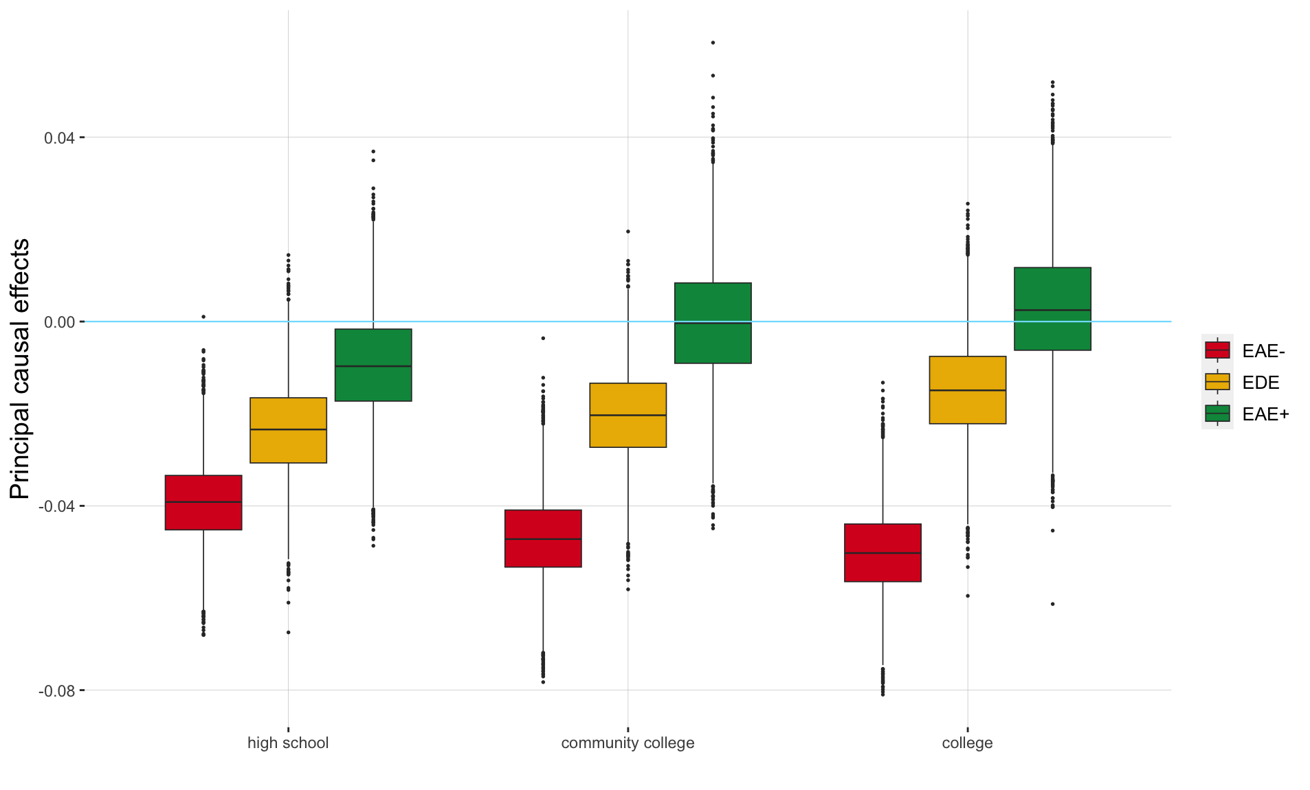
Overall, we can conclude that the pm2.5 exposure does have a negative effect on social mobility, coherently to the conclusion of Lee, Merlo and Dominici (2024). However, the effects are negative even for the dissociative strata, meaning that even when pm2.5 does not hinder educational attainments, the effects on social mobility are still negative. The principal causal effect has a bigger range when the intermediate variable is the college rate and a smaller range for the high school graduation rate.
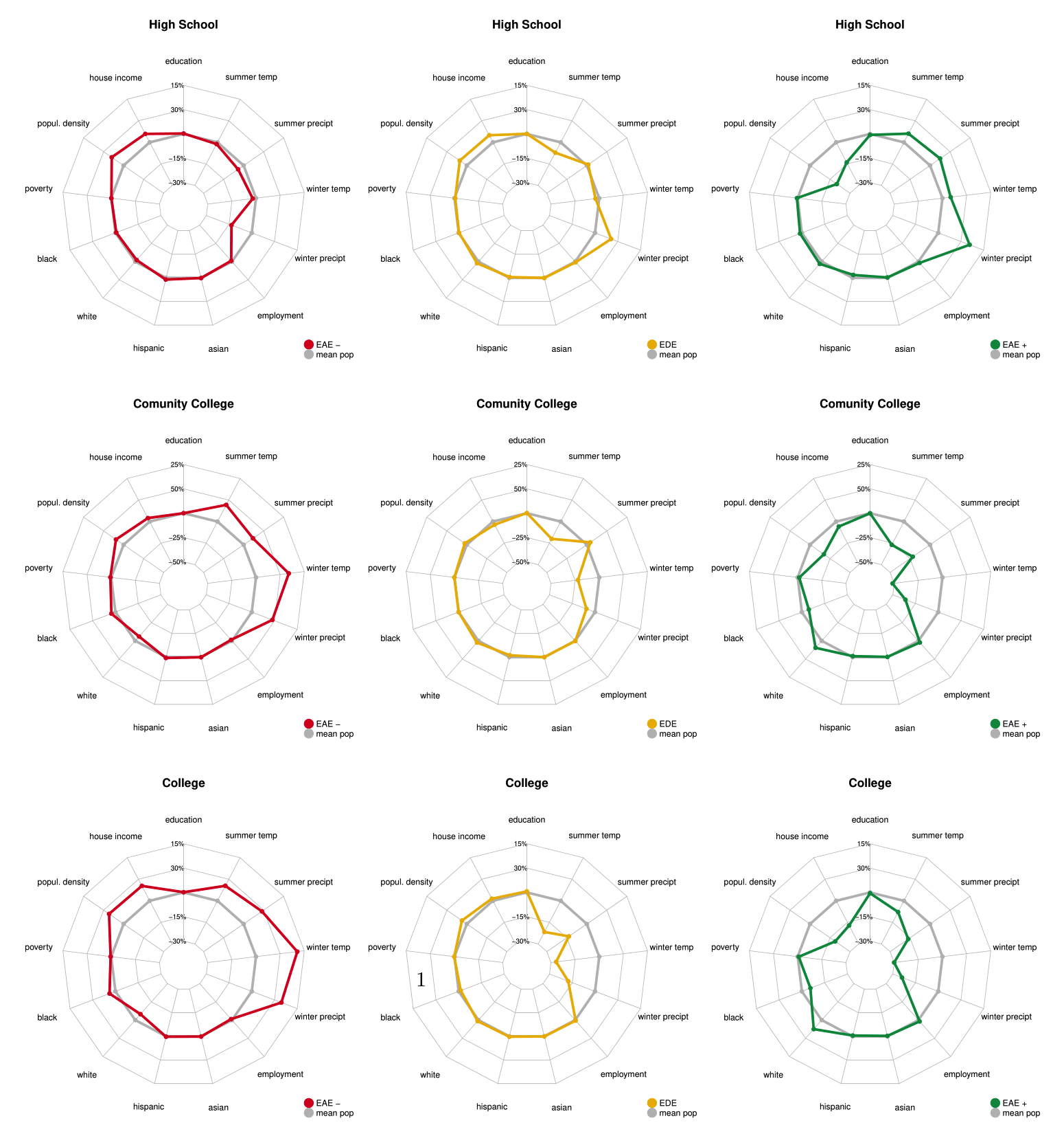
Analyzing the distribution of characteristics between strata provides insights for designing targeted social policies to promote equity within the population. Figure 2 highlights that the primary factors that differ between strata include weather conditions, population density, median household income, and ethnic composition (percentage of white and black populations).
Weather conditions exhibit varying patterns based on education levels: counties with higher temperatures and more rainfall are associated with the positive associative stratum when high school is the mediator of the causal effect of exposure to pm2.5 on social mobility. In contrast, for college and community college as mediators, these weather features define the negative associative stratum.
A consistent finding across the three levels of education is that counties with higher population density and higher median household income—typically urban areas—are more adversely affected by pm2.5 exposure, leading to significant reductions in social mobility (negative associative stratum). Furthermore, counties with a higher percentage of white residents are predominantly assigned to the positive associative stratum, aligning with literature that indicates that white populations are less affected by air pollution and are more likely to experience upward social mobility. In contrast, counties with a higher proportion of Black residents are concentrated in the negative associative stratum, emphasizing the need for targeted social policies to mitigate the increased risks faced by black populations, particularly in urban areas, due to air pollution.
7 Conclusion
In this paper, we propose a novel Bayesian approach for the principal stratification framework. The post-treatment variable plays a key role in defining causal effects in numerous real-world applications, where the primary challenge lies in the complexity of relationships among the involved variables.
Leveraging the DDP prior we defined a flexible model for this framework that allows us to (i) capture the heterogeneity in the potential outcomes, (ii) correctly input the missing data, both in the post-treatment variable and in the final outcome, and (iii) estimate the principal causal effects.
The performance of the proposed model was evaluated in the simulation study, where we compared it with the state-of-the-art BNP model for principal stratification. Having tested for different levels of heterogeneity in the potential outcome for the post-treatment variable and for the final outcome, the proposed model depicted a better performance than the model proposed by Schwartz, Li and Mealli (2011). The latter’s mixture model captures the heterogeneity in the post-treatment variable comparably to our model—see Scenario 1 for the post-treatment variable—while our model, with a mixture distribution for the final outcome, improves the performance on the final outcome whether it is with or without heterogeneity.
An illustrative example, we studied the principal causal effects of air pollution on social mobility—where education level served as a post-treatment variable that is an intermediary between air pollution and social mobility—exhibiting different patterns depending on the different principal strata. In this motivating application, we were interested in capturing the causal effects of pm2.5 exposure on social mobility in three strata: the counties where pm2.5 exposure does not alter education levels and the two associative strata where, in opposition, education levels decrease or improve when exposed to a higher level of pm2.5Overall, the results revealed a consistent negative relationship between pm2.5 exposure and social mobility for all of three education levels—high school, community college, and college rate—that served as a post-treatment variable. The heterogeneity in principal causal effects showed similar patterns across the three education levels. The higher pm2.5 exposure reduces the education rate in the population, which in turn reduces social mobility. In counties where the level of education increases with the higher level of pm2.5 , no significant causal effect is measured in social mobility.
This work is the first to study this complex causal link between air pollution and social mobility when the education level serves as an intermediate variable. Future research could investigate different post-treatment variables or consider simultaneously multiple ones.
From a methodological perspective, our approach can be extended by integrating our model with those proposed by Schwartz, Li and Mealli (2011) or Zorzetto et al. (2024a). Such integration would facilitate the formulation of a fully Bayesian nonparametric framework utilizing a DDP prior for the parameters governing the distributions of the post-treatment variable and the final outcome. Additionally, incorporating the prior introduced by Zorzetto et al. (2024a) would enable the estimation of the principal strata without threshold assumptions, allowing the data to guide the strata partitioning process. We leave this to future research.
[Acknowledgments] The authors wish to thank Luca Merlo and Sophie-An Kingsbury Lee for their helpful suggestions and comments for the application. {funding} This work was partially funded by the following grants: NIH: R01ES026217, R01MD012769, R01ES028033, 1R01ES030616, 1R01AG066793, 1R01MD016054-01A1; Sloan Foundation: G-2020-13946.
Supplement to ’Disentangling the Effects of Air Pollution on Social Mobility: A Bayesian Principal Stratification Approach’ \sdescriptionFurther details for the simulation study described in Section 5 are reported in Appendix A and B, respectively about the data generation process and the results visualization. The posterior distribution and the Gibbs sampler for the model introduced in Section 4 is in Appendix C.
Code \sdescriptionCode for implementing the proposed model and for replicating the results of simulation study and application is publicly available at https://github.com/dafzorzetto/StrataBayes.
Data \sdescriptionThe data are available at the original dataset, and the indication to obtain the analyzed dataset are reported at https://github.com/dafzorzetto/StrataBayes.
References
- Angrist, Imbens and Rubin (1996) {barticle}[author] \bauthor\bsnmAngrist, \bfnmJoshua D\binitsJ. D., \bauthor\bsnmImbens, \bfnmGuido W\binitsG. W. and \bauthor\bsnmRubin, \bfnmDonald B\binitsD. B. (\byear1996). \btitleIdentification of causal effects using instrumental variables. \bjournalJournal of the American Statistical Association \bvolume91 \bpages444–455. \endbibitem
- Antonelli et al. (2023) {barticle}[author] \bauthor\bsnmAntonelli, \bfnmJoseph\binitsJ., \bauthor\bsnmMealli, \bfnmFabrizia\binitsF., \bauthor\bsnmBeck, \bfnmBrenden\binitsB. and \bauthor\bsnmMattei, \bfnmAlessandra\binitsA. (\byear2023). \btitlePrincipal stratification with continuous treatments and continuous post-treatment variables. \bjournalarXiv preprint arXiv:2309.14486. \endbibitem
- Bargagli-Stoffi et al. (2020) {barticle}[author] \bauthor\bsnmBargagli-Stoffi, \bfnmFalco J\binitsF. J., \bauthor\bsnmCadei, \bfnmRiccardo\binitsR., \bauthor\bsnmLee, \bfnmKwonsang\binitsK. and \bauthor\bsnmDominici, \bfnmFrancesca\binitsF. (\byear2020). \btitleCausal Rule Ensemble: Interpretable Discovery and Inference of Heterogeneous Causal Effects. \bjournalarXiv preprint arXiv:2009.09036. \endbibitem
- Barrientos, Jara and Quintana (2012) {barticle}[author] \bauthor\bsnmBarrientos, \bfnmAndrés F\binitsA. F., \bauthor\bsnmJara, \bfnmAlejandro\binitsA. and \bauthor\bsnmQuintana, \bfnmFernando A\binitsF. A. (\byear2012). \btitleOn the support of MacEachern’s dependent Dirichlet processes and extensions. \bjournalBayesian Analysis \bvolume7 \bpages277–310. \endbibitem
- Bell and Ebisu (2012) {barticle}[author] \bauthor\bsnmBell, \bfnmMichelle L\binitsM. L. and \bauthor\bsnmEbisu, \bfnmKeita\binitsK. (\byear2012). \btitleEnvironmental inequality in exposures to airborne particulate matter components in the United States. \bjournalEnvironmental health perspectives \bvolume120 \bpages1699-1704. \endbibitem
- Binelli, Loveless and Whitefield (2015) {barticle}[author] \bauthor\bsnmBinelli, \bfnmChiara\binitsC., \bauthor\bsnmLoveless, \bfnmMatthew\binitsM. and \bauthor\bsnmWhitefield, \bfnmStephen\binitsS. (\byear2015). \btitleWhat Is Social Inequality and Why Does it Matter? Evidence from Central and Eastern Europe. \bjournalWorld Development \bvolume70 \bpages239-248. \bdoihttps://doi.org/10.1016/j.worlddev.2015.02.007 \endbibitem
- Blanden et al. (2014) {bbook}[author] \bauthor\bsnmBlanden, \bfnmJoanne\binitsJ., \bauthor\bsnmMacmillan, \bfnmLindsey\binitsL. \betalet al. (\byear2014). \btitleEducation and Intergenerational Mobility: Help Or Hinderence? \bpublisherCentre for Analysis of Social Exclusion. \endbibitem
- Braithwaite et al. (2019) {barticle}[author] \bauthor\bsnmBraithwaite, \bfnmIsobel\binitsI., \bauthor\bsnmZhang, \bfnmShuo\binitsS., \bauthor\bsnmKirkbride, \bfnmJames B\binitsJ. B., \bauthor\bsnmOsborn, \bfnmDavid PJ\binitsD. P. and \bauthor\bsnmHayes, \bfnmJoseph F\binitsJ. F. (\byear2019). \btitleAir pollution (particulate matter) exposure and associations with depression, anxiety, bipolar, psychosis and suicide risk: a systematic review and meta-analysis. \bjournalEnvironmental health perspectives \bvolume127 \bpages126002. \endbibitem
- Brochu et al. (2011) {barticle}[author] \bauthor\bsnmBrochu, \bfnmPaul J\binitsP. J., \bauthor\bsnmYanosky, \bfnmJeff D\binitsJ. D., \bauthor\bsnmPaciorek, \bfnmChristopher J\binitsC. J., \bauthor\bsnmSchwartz, \bfnmJoel\binitsJ., \bauthor\bsnmChen, \bfnmJarvis T\binitsJ. T., \bauthor\bsnmHerrick, \bfnmRobert F\binitsR. F. and \bauthor\bsnmSuh, \bfnmHelen H\binitsH. H. (\byear2011). \btitleParticulate air pollution and socioeconomic position in rural and urban areas of the Northeastern United States. \bjournalAmerican journal of public health \bvolume101 \bpagesS224–S230. \endbibitem
- Brown and James (2020) {barticle}[author] \bauthor\bsnmBrown, \bfnmPhillip\binitsP. and \bauthor\bsnmJames, \bfnmDavid\binitsD. (\byear2020). \btitleEducational expansion, poverty reduction and social mobility: Reframing the debate. \bjournalInternational Journal of Educational Research \bvolume100 \bpages101537. \endbibitem
- Card (2001) {barticle}[author] \bauthor\bsnmCard, \bfnmDavid\binitsD. (\byear2001). \btitleEstimating the return to schooling: Progress on some persistent econometric problems. \bjournalEconometrica \bvolume69 \bpages1127–1160. \endbibitem
- Castro, Yazdi and Schwartz (2024) {bmisc}[author] \bauthor\bsnmCastro, \bfnmE.\binitsE., \bauthor\bsnmYazdi, \bfnmM. Danesh\binitsM. D. and \bauthor\bsnmSchwartz, \bfnmJ.\binitsJ. (\byear2024). \btitleDaymet v4 daily surface weather aggregated to TIGER/Line geographies. \bnoteAccessed: 20 August 2024. \bdoi10.7910/DVN/MRZGNQ \endbibitem
- Chetty et al. (2017) {barticle}[author] \bauthor\bsnmChetty, \bfnmRaj\binitsR., \bauthor\bsnmGrusky, \bfnmDavid\binitsD., \bauthor\bsnmHell, \bfnmMaximilian\binitsM., \bauthor\bsnmHendren, \bfnmNathaniel\binitsN., \bauthor\bsnmManduca, \bfnmRobert\binitsR. and \bauthor\bsnmNarang, \bfnmJimmy\binitsJ. (\byear2017). \btitleThe fading American dream: Trends in absolute income mobility since 1940. \bjournalScience \bvolume356 \bpages398–406. \endbibitem
- Chetty et al. (2018) {btechreport}[author] \bauthor\bsnmChetty, \bfnmRaj\binitsR., \bauthor\bsnmFriedman, \bfnmJohn N\binitsJ. N., \bauthor\bsnmHendren, \bfnmNathaniel\binitsN., \bauthor\bsnmJones, \bfnmMaggie R\binitsM. R. and \bauthor\bsnmPorter, \bfnmSonya R\binitsS. R. (\byear2018). \btitleThe opportunity atlas: Mapping the childhood roots of social mobility \btypeTechnical Report, \bpublisherNational Bureau of Economic Research. \endbibitem
- Choi, Kim and Kim (2023) {barticle}[author] \bauthor\bsnmChoi, \bfnmYoung Jun\binitsY. J., \bauthor\bsnmKim, \bfnmJi Hyun\binitsJ. H. and \bauthor\bsnmKim, \bfnmYun Young\binitsY. Y. (\byear2023). \btitleSocial Mobility from a Gender Perspective: Dynamics of Mothers’ Roles in Daughters’ Labor Market Performance. \bjournalSocial Indicators Research \bvolume168 \bpages119–138. \endbibitem
- Colmer, Voorheis and Williams (2023) {bmisc}[author] \bauthor\bsnmColmer, \bfnmJ.\binitsJ., \bauthor\bsnmVoorheis, \bfnmJ.\binitsJ. and \bauthor\bsnmWilliams, \bfnmB.\binitsB. (\byear2023). \btitleAir pollution and economic opportunity in the United States. \endbibitem
- Conlon, Taylor and Elliott (2014) {barticle}[author] \bauthor\bsnmConlon, \bfnmAnna SC\binitsA. S., \bauthor\bsnmTaylor, \bfnmJeremy MG\binitsJ. M. and \bauthor\bsnmElliott, \bfnmMichael R\binitsM. R. (\byear2014). \btitleSurrogacy assessment using principal stratification when surrogate and outcome measures are multivariate normal. \bjournalBiostatistics \bvolume15 \bpages266–283. \endbibitem
- Connor and Storper (2020) {barticle}[author] \bauthor\bsnmConnor, \bfnmDylan Shane\binitsD. S. and \bauthor\bsnmStorper, \bfnmMichael\binitsM. (\byear2020). \btitleThe changing geography of social mobility in the United States. \bjournalProceedings of the National Academy of Sciences \bvolume117 \bpages30309–30317. \endbibitem
- Currie, Neidell and Schmieder (2009) {barticle}[author] \bauthor\bsnmCurrie, \bfnmJanet\binitsJ., \bauthor\bsnmNeidell, \bfnmMatthew\binitsM. and \bauthor\bsnmSchmieder, \bfnmJohannes F\binitsJ. F. (\byear2009). \btitleAir pollution and infant health: Lessons from New Jersey. \bjournalJournal of health economics \bvolume28 \bpages688–703. \endbibitem
- Ding et al. (2017) {barticle}[author] \bauthor\bsnmDing, \bfnmPeng\binitsP., \bauthor\bsnmLu, \bfnmJiannan\binitsJ. \betalet al. (\byear2017). \btitlePrincipal stratification analysis using principal scores. \bjournalJournal of the Royal Statistical Society Series B \bvolume79 \bpages757–777. \endbibitem
- Feller, Mealli and Miratrix (2017) {barticle}[author] \bauthor\bsnmFeller, \bfnmAvi\binitsA., \bauthor\bsnmMealli, \bfnmFabrizia\binitsF. and \bauthor\bsnmMiratrix, \bfnmLuke\binitsL. (\byear2017). \btitlePrincipal score methods: Assumptions, extensions, and practical considerations. \bjournalJournal of Educational and Behavioral Statistics \bvolume42 \bpages726–758. \endbibitem
- Ferguson (1973) {barticle}[author] \bauthor\bsnmFerguson, \bfnmThomas S\binitsT. S. (\byear1973). \btitleA Bayesian analysis of some nonparametric problems. \bjournalThe Annals of Statistics \bpages209–230. \endbibitem
- Frangakis and Rubin (2002) {barticle}[author] \bauthor\bsnmFrangakis, \bfnmConstantine E\binitsC. E. and \bauthor\bsnmRubin, \bfnmDonald B\binitsD. B. (\byear2002). \btitlePrincipal stratification in causal inference. \bjournalBiometrics \bvolume58 \bpages21–29. \endbibitem
- Grunewald et al. (2017) {barticle}[author] \bauthor\bsnmGrunewald, \bfnmNicole\binitsN., \bauthor\bsnmKlasen, \bfnmStephan\binitsS., \bauthor\bsnmMartínez-Zarzoso, \bfnmInmaculada\binitsI. and \bauthor\bsnmMuris, \bfnmChris\binitsC. (\byear2017). \btitleThe Trade-off Between Income Inequality and Carbon Dioxide Emissions. \bjournalEcological Economics \bvolume142 \bpages249-256. \bdoihttps://doi.org/10.1016/j.ecolecon.2017.06.034 \endbibitem
- Hajat, Hsia and O’Neill (2015) {barticle}[author] \bauthor\bsnmHajat, \bfnmAnjum\binitsA., \bauthor\bsnmHsia, \bfnmCharlene\binitsC. and \bauthor\bsnmO’Neill, \bfnmMarie S\binitsM. S. (\byear2015). \btitleSocioeconomic disparities and air pollution exposure: a global review. \bjournalCurrent environmental health reports \bvolume2 \bpages440-450. \endbibitem
- Heckman and Landersø (2022) {barticle}[author] \bauthor\bsnmHeckman, \bfnmJames\binitsJ. and \bauthor\bsnmLandersø, \bfnmRasmus\binitsR. (\byear2022). \btitleLessons for Americans from Denmark about inequality and social mobility. \bjournalLabour economics \bvolume77 \bpages101999. \endbibitem
- Holland (1986) {barticle}[author] \bauthor\bsnmHolland, \bfnmPaul W\binitsP. W. (\byear1986). \btitleStatistics and causal inference. \bjournalJournal of the American Statistical Association \bvolume81 \bpages945–960. \endbibitem
- Jiang, Yang and Ding (2022) {barticle}[author] \bauthor\bsnmJiang, \bfnmZhichao\binitsZ., \bauthor\bsnmYang, \bfnmShu\binitsS. and \bauthor\bsnmDing, \bfnmPeng\binitsP. (\byear2022). \btitleMultiply robust estimation of causal effects under principal ignorability. \bjournalJournal of the Royal Statistical Society Series B: Statistical Methodology \bvolume84 \bpages1423–1445. \endbibitem
- Jin and Rubin (2008) {barticle}[author] \bauthor\bsnmJin, \bfnmHui\binitsH. and \bauthor\bsnmRubin, \bfnmDonald B\binitsD. B. (\byear2008). \btitlePrincipal stratification for causal inference with extended partial compliance. \bjournalJournal of the American Statistical Association \bvolume103 \bpages101–111. \endbibitem
- Kim and Zigler (2024) {barticle}[author] \bauthor\bsnmKim, \bfnmChanmin\binitsC. and \bauthor\bsnmZigler, \bfnmCorwin\binitsC. (\byear2024). \btitleBayesian Nonparametric Trees for Principal Causal Effects. \bjournalarXiv preprint arXiv:2403.13256. \endbibitem
- Lee, Merlo and Dominici (2024) {barticle}[author] \bauthor\bsnmLee, \bfnmSophie-An Kingsbury\binitsS.-A. K., \bauthor\bsnmMerlo, \bfnmLuca\binitsL. and \bauthor\bsnmDominici, \bfnmFrancesca\binitsF. (\byear2024). \btitleChildhood PM2.5 exposure and upward mobility in the United States. \bjournalProceedings of the National Academy of Sciences \bvolume121 \bpagese2401882121. \endbibitem
- Lee, Small and Dominici (2021) {barticle}[author] \bauthor\bsnmLee, \bfnmKwonsang\binitsK., \bauthor\bsnmSmall, \bfnmDylan S\binitsD. S. and \bauthor\bsnmDominici, \bfnmFrancesca\binitsF. (\byear2021). \btitleDiscovering heterogeneous exposure effects using randomization inference in air pollution studies. \bjournalJournal of the American Statistical Association \bvolume116 \bpages569–580. \endbibitem
- Lu, Jiang and Ding (2023) {barticle}[author] \bauthor\bsnmLu, \bfnmSizhu\binitsS., \bauthor\bsnmJiang, \bfnmZhichao\binitsZ. and \bauthor\bsnmDing, \bfnmPeng\binitsP. (\byear2023). \btitlePrincipal Stratification with Continuous Post-Treatment Variables: Nonparametric Identification and Semiparametric Estimation. \bjournalarXiv preprint arXiv:2309.12425. \endbibitem
- MacEachern (2000) {barticle}[author] \bauthor\bsnmMacEachern, \bfnmSteven N\binitsS. N. (\byear2000). \btitleDependent Dirichlet processes. Technical Report. \bjournalDepartment of Statistics, The Ohio State University, Columbus, OH. \endbibitem
- Mealli and Mattei (2012) {barticle}[author] \bauthor\bsnmMealli, \bfnmFabrizia\binitsF. and \bauthor\bsnmMattei, \bfnmAlessandra\binitsA. (\byear2012). \btitleA refreshing account of principal stratification. \bjournalThe International Journal of Biostatistics \bvolume8. \endbibitem
- Mohai et al. (2011) {barticle}[author] \bauthor\bsnmMohai, \bfnmPaul\binitsP., \bauthor\bsnmKweon, \bfnmByoung-Suk\binitsB.-S., \bauthor\bsnmLee, \bfnmSangyun\binitsS. and \bauthor\bsnmArd, \bfnmKerry\binitsK. (\byear2011). \btitleAir pollution around schools is linked to poorer student health and academic performance. \bjournalHealth Affairs \bvolume30 \bpages852–862. \endbibitem
- Pfeffer and Hertel (2015) {barticle}[author] \bauthor\bsnmPfeffer, \bfnmFabian T\binitsF. T. and \bauthor\bsnmHertel, \bfnmFlorian R\binitsF. R. (\byear2015). \btitleHow Has Educational Expansion Shaped Social Mobility Trends in the United States? \bjournalSocial Forces \bvolume94 \bpages143–180. \bdoi10.1093/sf/sov045 \endbibitem
- Piketty, Saez and Zucman (2018) {barticle}[author] \bauthor\bsnmPiketty, \bfnmThomas\binitsT., \bauthor\bsnmSaez, \bfnmEmmanuel\binitsE. and \bauthor\bsnmZucman, \bfnmGabriel\binitsG. (\byear2018). \btitleDistributional national accounts: methods and estimates for the United States. \bjournalThe Quarterly Journal of Economics \bvolume133 \bpages553–609. \endbibitem
- Platt (2019) {bbook}[author] \bauthor\bsnmPlatt, \bfnmLucinda\binitsL. (\byear2019). \btitleUnderstanding inequalities: Stratification and difference. \bpublisherJohn Wiley & Sons. \endbibitem
- Quintana et al. (2022) {barticle}[author] \bauthor\bsnmQuintana, \bfnmFernand A\binitsF. A., \bauthor\bsnmMueller, \bfnmPeter\binitsP., \bauthor\bsnmJara, \bfnmAlejandro\binitsA. and \bauthor\bsnmMacEachern, \bfnmSteven N\binitsS. N. (\byear2022). \btitleThe dependent Dirichlet process and related models. \bjournalStatistical Science \bvolume37 \bpages24–41. \endbibitem
- Rodriguez and Dunson (2011) {barticle}[author] \bauthor\bsnmRodriguez, \bfnmAbel\binitsA. and \bauthor\bsnmDunson, \bfnmDavid B\binitsD. B. (\byear2011). \btitleNonparametric Bayesian models through probit stick-breaking processes. \bjournalBayesian Analysis (Online) \bvolume6. \endbibitem
- Rubin (1974a) {barticle}[author] \bauthor\bsnmRubin, \bfnmDonald B\binitsD. B. (\byear1974a). \btitleEstimating causal effects of treatments in randomized and nonrandomized studies. \bjournalJournal of Educational Psychology \bvolume66 \bpages688. \endbibitem
- Rubin (1974b) {barticle}[author] \bauthor\bsnmRubin, \bfnmDonald B\binitsD. B. (\byear1974b). \btitleEstimating causal effects of treatments in randomized and nonrandomized studies. \bjournalJournal of Educational Psychology \bvolume66 \bpages688. \endbibitem
- Rubin (1986) {barticle}[author] \bauthor\bsnmRubin, \bfnmDonald B\binitsD. B. (\byear1986). \btitleComment: Which ifs have causal answers. \bjournalJournal of the American Statistical Association \bvolume81 \bpages961–962. \endbibitem
- Salvanes (2023) {barticle}[author] \bauthor\bsnmSalvanes, \bfnmKjell G\binitsK. G. (\byear2023). \btitleWhat Drives Intergenerational Mobility? The Role of Family, Neighborhood, Education, and Social Class: A Review of Bukodi and Goldthorpe’s Social Mobility and Education in Britain. \bjournalJournal of Economic Literature \bvolume61 \bpages1540–1578. \endbibitem
- Schwartz, Li and Mealli (2011) {barticle}[author] \bauthor\bsnmSchwartz, \bfnmScott L\binitsS. L., \bauthor\bsnmLi, \bfnmFan\binitsF. and \bauthor\bsnmMealli, \bfnmFabrizia\binitsF. (\byear2011). \btitleA Bayesian semiparametric approach to intermediate variables in causal inference. \bjournalJournal of the American Statistical Association \bvolume106 \bpages1331–1344. \endbibitem
- Sethuraman (1994) {barticle}[author] \bauthor\bsnmSethuraman, \bfnmJayaram\binitsJ. (\byear1994). \btitleA constructive definition of Dirichlet priors. \bjournalStatistica Sinica \bpages639–650. \endbibitem
- Shehab and Pope (2019) {barticle}[author] \bauthor\bsnmShehab, \bfnmMA\binitsM. and \bauthor\bsnmPope, \bfnmFD\binitsF. (\byear2019). \btitleEffects of short-term exposure to particulate matter air pollution on cognitive performance. \bjournalScientific reports \bvolume9 \bpages8237. \endbibitem
- Sjölander et al. (2009) {barticle}[author] \bauthor\bsnmSjölander, \bfnmArvid\binitsA., \bauthor\bsnmHumphreys, \bfnmKeith\binitsK., \bauthor\bsnmVansteelandt, \bfnmStijn\binitsS., \bauthor\bsnmBellocco, \bfnmRino\binitsR. and \bauthor\bsnmPalmgren, \bfnmJuni\binitsJ. (\byear2009). \btitleSensitivity analysis for principal stratum direct effects, with an application to a study of physical activity and coronary heart disease. \bjournalBiometrics \bvolume65 \bpages514–520. \endbibitem
- Song et al. (2019) {barticle}[author] \bauthor\bsnmSong, \bfnmJae\binitsJ., \bauthor\bsnmPrice, \bfnmDavid J\binitsD. J., \bauthor\bsnmGuvenen, \bfnmFatih\binitsF., \bauthor\bsnmBloom, \bfnmNicholas\binitsN. and \bauthor\bsnmVon Wachter, \bfnmTill\binitsT. (\byear2019). \btitleFirming up inequality. \bjournalThe Quarterly Journal of Economics \bvolume134 \bpages1–50. \endbibitem
- Stiglitz (2012) {bbook}[author] \bauthor\bsnmStiglitz, \bfnmJoseph E\binitsJ. E. (\byear2012). \btitleThe price of inequality: How today’s divided society endangers our future. \bpublisherWW Norton & Company, \baddressNew York. \endbibitem
- Sunyer et al. (2015) {barticle}[author] \bauthor\bsnmSunyer, \bfnmJordi\binitsJ., \bauthor\bsnmEsnaola, \bfnmMikel\binitsM., \bauthor\bsnmAlvarez-Pedrerol, \bfnmMar\binitsM., \bauthor\bsnmForns, \bfnmJoan\binitsJ., \bauthor\bsnmRivas, \bfnmIoar\binitsI., \bauthor\bsnmL’opez-Vicente, \bfnmM‘onica\binitsM., \bauthor\bsnmSuades-Gonz’alez, \bfnmElisabet\binitsE., \bauthor\bsnmForaster, \bfnmMaria\binitsM., \bauthor\bsnmGarcia-Esteban, \bfnmRaquel\binitsR., \bauthor\bsnmBasaga na, \bfnmXavier\binitsX. \betalet al. (\byear2015). \btitleAssociation between traffic-related air pollution in schools and cognitive development in primary school children: a prospective cohort study. \bjournalPLoS medicine \bvolume12 \bpagese1001792. \endbibitem
- Van Bavel et al. (2011) {barticle}[author] \bauthor\bsnmVan Bavel, \bfnmJan\binitsJ., \bauthor\bsnmMoreels, \bfnmSarah\binitsS., \bauthor\bparticleVan de \bsnmPutte, \bfnmBart\binitsB. and \bauthor\bsnmMatthijs, \bfnmKoen\binitsK. (\byear2011). \btitleFamily size and intergenerational social mobility during the fertility transition: Evidence of resource dilution from the city of Antwerp in nineteenth century Belgium. \bjournalDemographic Research \bvolume24 \bpages313–344. \endbibitem
- VanderWeele (2011) {barticle}[author] \bauthor\bsnmVanderWeele, \bfnmTyler J\binitsT. J. (\byear2011). \btitlePrincipal stratification–uses and limitations. \bjournalThe International Journal of Biostatistics \bvolume7 \bpages1–14. \endbibitem
- Yang and Liu (2018) {barticle}[author] \bauthor\bsnmYang, \bfnmTingru\binitsT. and \bauthor\bsnmLiu, \bfnmWenling\binitsW. (\byear2018). \btitleDoes air pollution affect public health and health inequality? Empirical evidence from China. \bjournalJournal of Cleaner Production \bvolume203 \bpages43-52. \bdoihttps://doi.org/10.1016/j.jclepro.2018.08.242 \endbibitem
- Zhang, Chen and Zhang (2018) {barticle}[author] \bauthor\bsnmZhang, \bfnmXin\binitsX., \bauthor\bsnmChen, \bfnmXi\binitsX. and \bauthor\bsnmZhang, \bfnmXiaobo\binitsX. (\byear2018). \btitleThe impact of exposure to air pollution on cognitive performance. \bjournalProceedings of the National Academy of Sciences \bvolume115 \bpages9193–9197. \endbibitem
- Zigler, Choirat and Dominici (2018) {barticle}[author] \bauthor\bsnmZigler, \bfnmCorwin M\binitsC. M., \bauthor\bsnmChoirat, \bfnmChristine\binitsC. and \bauthor\bsnmDominici, \bfnmFrancesca\binitsF. (\byear2018). \btitleImpact of National Ambient Air Quality Standards nonattainment designations on particulate pollution and health. \bjournalEpidemiology (Cambridge, Mass.) \bvolume29 \bpages165. \endbibitem
- Zorzetto et al. (2024a) {barticle}[author] \bauthor\bsnmZorzetto, \bfnmDafne\binitsD., \bauthor\bsnmCanale, \bfnmAntonio\binitsA., \bauthor\bsnmMealli, \bfnmFabrizia\binitsF., \bauthor\bsnmDominici, \bfnmFrancesca\binitsF. and \bauthor\bsnmBargagli-Stoffi, \bfnmFalco J\binitsF. J. (\byear2024a). \btitleBayesian Nonparametrics for Principal Stratification with Continuous Post-Treatment Variables. \bjournalarXiv preprint arXiv:2405.17669. \endbibitem
- Zorzetto et al. (2024b) {barticle}[author] \bauthor\bsnmZorzetto, \bfnmDafne\binitsD., \bauthor\bsnmBargagli-Stoffi, \bfnmFalco J\binitsF. J., \bauthor\bsnmCanale, \bfnmAntonio\binitsA. and \bauthor\bsnmDominici, \bfnmFrancesca\binitsF. (\byear2024b). \btitleConfounder-dependent Bayesian mixture model: Characterizing heterogeneity of causal effects in air pollution epidemiology. \bjournalBiometrics \bvolume80 \bpagesujae025. \endbibitem