CHARACTERIZATION OF SMOOTH SOLUTIONS TO THE NAVIER-STOKES EQUATIONS IN A PIPE WITH TWO TYPES OF SLIP BOUNDARY CONDITIONS

The 3D stationary Navier-Stokes (NS) equations which describes the motion of stationary viscous incompressible fluids follows that

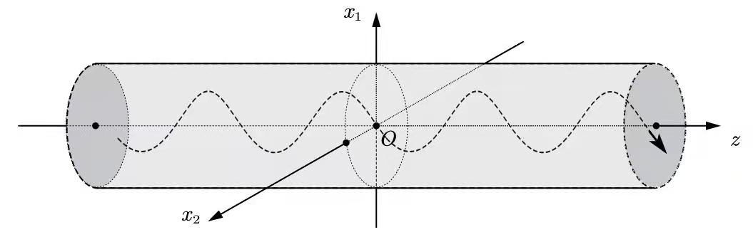
Here $u(x)\in\mathbb{R}^{3}$, $p(x)\in\mathbb{R}$ represents the velocity and the scalar pressure respectively. In this paper, we consider the domain $\mathcal{D}$ to be an infinitely long pipe, i.e.

where $x=(x_{1},x_{2},x_{3})$, $x_{h}=(x_{1},x_{2})$ and $|x_{h}|=\sqrt{x^{2}_{1}+x^{2}_{2}}$. The boundary condition will be equipped with the following:

Here $\mathbb{S}u=\frac{1}{2}\left(\nabla u+(\nabla u)^{T}\right)$ is the stress tensor, where $(\nabla u)^{T}$ is the transpose of the Jacobian matrix $\nabla u$, and $\boldsymbol{n}$ is the unit outer normal vector of $\partial\mathcal{D}$. For a vector field $v$, $v_{\tau}$ stands for its tangential part: $v_{\tau}:=v-(v\cdot\boldsymbol{n})\boldsymbol{n}.$ The condition (NSB) is from the general Navier-slip boundary condition and impermeable boundary condition which was introduced by Claude-Louis Naiver in 1820s [28]:

Here $\alpha\geq 0$ stands for the friction constant which may depend on various elements, such as the property of the boundary and the viscosity of the fluid. When $\alpha=0$, boundary condition (1.2) turns to the total Navier-slip boundary (NSB), and when $\alpha\to\infty$, boundary condition (1.2) degenerates into the no-slip boundary condition $u\equiv 0$ on the boundary.

The boundary condition (NHLB) is a special case in a family of boundary conditions proposed by Navier [28], which has been studied extensively in the literature and was attributed to different authors. The boundary condition was called the Navier-Hodge boundary condition in [25] and the Navier-Lions boundary condition in [23]. For this reason, we will call it the Navier-Hodge-Lions boundary condition in this paper.

We write $\mathcal{D}$ to be

where the cross section $\Sigma\in{\mathbb{R}}^{2}$ is a unit disc. The domain considered here is a high-degree simplification of the following “distorted cylinder”, i.e.

where $\tilde{\Sigma}\in{\mathbb{R}}^{2}$ is a simply connected bounded domain with smooth boundary.

Let $\tilde{\mathcal{D}}_{0}$ be a simply connected bounded domain with smooth boundary in ${\mathbb{R}}^{3}$ and $\tilde{\mathcal{D}}_{0}\cap\tilde{\mathcal{D}}\neq\emptyset$. Existence problem of weak solutions in domain $\tilde{\mathcal{D}}_{\text{Union}}:=\tilde{\mathcal{D}}\cup\tilde{\mathcal{D}}_{0}$ with the Navier-slip boundary (NSB) was addressed in [17] and regularity of solutions was also implied there. On the other hand, if $\tilde{\mathcal{D}}_{0}\subset\tilde{\mathcal{D}}$ is an “obstacle” in $\tilde{\mathcal{D}}$, then the two dimensional existence problems and asymptotic behaviors of smooth solutions in domain $\tilde{\mathcal{D}}_{\text{Diff}}:=\tilde{\mathcal{D}}\backslash\tilde{\mathcal{D}}_{0}$ with the total Navier-slip boundary condition are obtained in [26, 27].

There have also been many pieces of literature in studying the existence, uniqueness and asymptotic behavior of the Navier-Stokes equations in a distorted pipe $\tilde{\mathcal{D}}_{\text{Union}}$ or $\tilde{\mathcal{D}}_{\text{Diff}}$ with no-slip boundary and with the Poiseuille flow as the asymptotic profile at infinity (Leray’s problem: Ladyzhenskaya [18, p. 77] and [19, p. 551]). The first remarkable contribution on the solvability of Leray’s problem is due to Amick [1, 2], who reduced the solvability problem to the resolution of a variational problem related to the stability of the Poiseuille flow in a flat cylinder. However, uniqueness and existence of solutions with large flux are left open. Ladyzhenskaya and Solonnikov [20] gave a detailed analysis of this problem on existence, uniqueness and asymptotic behavior of small-flux solutions. One may refer to [3, 14, 30] and references for more details on well-posedness, decay and far-field asymptotic analysis of solutions for Leray’s problem and related topics. A systematic review and study of Leray’s problem can be found in [11, Chapter XIII]. Recently Wang-Xie in [33] studied uniform structural stability of Poiseuille flows for the 3D axially symmetric solutions in the 3D pipe $\mathcal{D}$ where a force term appears on the right hand of equation (1.1)₁.

Compared to the no-slip boundary condition, this model with the total Navier-slip or Navier-Hodge-Lions boundary condition has different physical interpretations and gives different mathematical properties. Literature [26, 17] addressed the existence and regularity problems of weak solutions for the total Navier-slip boundary condition in a pipe, but uniqueness was left open. Also readers can refer to, i.e., [4, 10, 23, 34] for some well-posedness results for the Navier-Hodge-Lions boundary condition in different domains. In this paper, we attempt to derive some uniqueness results for the Navier-Stokes equations with the total Navier-slip or Navier-Hodge-Lions boundary condition in the regular infinite pipe $\mathcal{D}$. We emphasize that our results below do not require any smallness and decay assumptions.

In this paper, for the boundary condition (NSB), a family of smooth helical solutions will be given, and for the Navier-Hodge-Lions boundary condition (NHLB), the trivial shear flow is easy to be discovered. We concern on the characterization and uniqueness of these two types of smooth solutions in $\mathcal{D}$.

Most of our proof will be carried out in the framework of cylindrical coordinates $(r,\theta,z)$ and some of our results are restricted to the axially symmetric solutions. Here we give the formulation of axially symmetric solutions in the cylindrical coordinates which enjoy the following relationship with 3D Euclidian coordinates:

A stationary axially symmetric solution of the incompressible Navier-Stokes equations is given as

where the basis vectors $\boldsymbol{e_{r}}$, $\boldsymbol{e_{\theta}}$ ,$\boldsymbol{e_{z}}$ are

while the components $u_{r},u_{\theta},u_{z}$, which are independent of $\theta$, satisfy

where $b=u_{r}\boldsymbol{e}_{r}+u_{z}\boldsymbol{e}_{z}$.

We can also compute the axi-symmetric vorticity $\omega=\nabla\times u=\omega_{r}\boldsymbol{e_{r}}+\omega_{\theta}\boldsymbol{e_{\theta}}+\omega_{z}\boldsymbol{e_{z}}$ as follows

which satisfies

In the cylindrical coordinates, the total Navier-slip boundary condition (NSB) is represented as

while the Navier-Hodge-Lions boundary condition (NHLB) is given by

whose computations are postponed to Appendix A.

Clearly direct calculation shows that, for arbitrary constants $C_{1}$ and $C_{2}$, the following type of helical solutions

solves (1.3) with the boundary condition (1.5).

We further note that helical solutions (1.7), which is smooth in $\mathcal{D}$, enjoys the following property:

Thus a natural question raises:

Are helical solutions (1.7) the only smooth solutions of system (1.3) with the boundary condition (1.5) which enjoys property ($\ast$ ‣ 1)?

Before answering this question, we recall that the flux $\Phi(z)$ at the cross section $\Sigma$, which is defined by

is a constant. Here $\boldsymbol{\nu}=\boldsymbol{e_{z}}$ is the unit normal vector of $\Sigma$ pointing to the positive $z$ direction. Actually by using the divergence free condition of the velocity and the boundary condition (NSB)₂, we have

where $\boldsymbol{n}=(n_{1},n_{2},0)$ is the unit outer normal vector of $\partial\mathcal{D}$. Then for any $z\in\mathbb{R}$, we will denote $\Phi(z)=\Phi$.

Our first result in this paper gives a positive answer to the above question in the following two cases:

• (i).

  the solution is axially symmetric and the flux $\Phi$ is zero (corresponding to $C_{2}=0$);

• (ii).

  the solution is $z$-periodic.

∎

Besides, we observe that solutions (1.7) enjoy the following property:

In the following theorem, we will conclude that if $u_{\theta}$ or $u_{z}$ is independent of $z$, then (1.7) are the only group of smooth solutions to (1.3) subject to the boundary condition (1.5).

In the case of $u_{\theta}$ being independent of $z$, the bounded $W^{1,\infty}$ assumption on the velocity will be extensively relaxed to the following:

for any $\gamma_{0}<\alpha\approx 3.83171$, $\delta_{0}<1$, and $M_{0}>0$. Here $\alpha$ is the first positive root of the Bessel function $J_{1}$. We recall that $J_{\beta}$ are canonical solutions of Bessel’s ordinary differential equation

which can be expressed by the following series form:

In the case of $u_{z}$ being independent of $z$, no size assumptions such as (1.9) are imposed on the solution.

∎

∎

∎

If we switch the total Navier-slip boundary condition to the Navier-Hodge-Lions boundary condition (NHLB), one notices that a non-zero swirling solution does not enjoy (NHLB). In this situation, one can derive the following Liouville-type theorem:

∎

There has already been much literature studying Liouville-type results on the Navier-Stokes equations subject to various boundary conditions in various unbounded domains. Readers can refer to [8, 9, 31, 32, 7, 29] and references therein for more Liouville-type results on the stationary Navier-Stokes equations. Moreover, our results in the above Theorems can be extended from the stationary case to the case of ancient solutions (backward global solutions) under suitable assumptions. However, for simplification of idea presenting, we omit this extension here and leave it to further works. See [13] where the authors established a Liouville-type result for the ancient solution to the Navier-Stokes equations in the half plane with the no-slip boundary condition.

Liouville-type results of ancient solutions is connected to the regularity of solutions to the initial value problem of the non-stationary Navier-Stokes equations. Type I blow-up solutions of the Navier-Stokes initial value problem could not exist provided the Liouville-type result holds for bounded ancient solutions. See [15, 12].

Before ending our introduction, we briefly outline our strategy for proofs of Theorem 1.1, Theorem 1.3 and Theorem 1.5. The most important ingredient of proving Theorem 1.1 is to show that $\mathbb{S}u\equiv 0$. For Case I in Theorem 1.1, we need to first show that $\mathbb{S}u\in L^{2}(\mathcal{D})$, which is not trivial since the pipe is an unbounded domain. In this process, $L^{\infty}$ oscillation boundedness of the pressure in $\mathcal{D}_{2Z}\backslash\mathcal{D}_{Z}$ (see (1.16) for the definition of $\mathcal{D}_{Z}$) is essential, which will be presented in Section 2.1.2. Then combining the square integrability of $\mathbb{S}u$ and boundedness of the velocity together with its gradient, a trick of integration by parts and Poincaré inequality will indicate that $u_{z}$ actually belongs to $L^{2}(\mathcal{D})$, which will result in the vanishing of $\mathbb{S}u$. While vanishing of $\mathbb{S}u$ in Case II of Theorem 1.1 is directly due to the $x_{3}$-periodic property by performing the energy estimate in a single period. However, in the process, we must be careful of handing of the pressure, which may not be $x_{3}$ periodic. After analyzing ingredients of $\mathbb{S}u$, we finally conclude the validity of Theorem 1.1.

The idea for proof of Theorem 1.3 is completely different from that of Theorem 1.1. Under the assumption of Case I in Theorem 1.3, we will see that the quantity $\Omega:=\omega_{\theta}/r$ satisfies a nice linear elliptic equation with an advection term. Under the growing assumption (1.9) in domain $\mathcal{D}$, by using the Nash-Moser iteration, we can show that actually $\Omega\equiv 0$, which indicates that $b=u_{r}\boldsymbol{e_{r}}+u_{z}\boldsymbol{e_{z}}$ must be harmonic in $\mathcal{D}$. Then by constructing a barrier function, applying maximum principle and assumptions on $b$, one derives $u_{r}\equiv 0$ and $u_{z}$ must be a constant. From then on, (1.3)₂ is reduced to a linear ordinary differential equation of $u_{\theta}$, and we finally obtain $u_{\theta}=C_{1}r$. While under the assumption of Case II in Theorem 1.3, a rather direct computation implies that $u_{r}\equiv 0$ by using the divergence-free condition. Then by combining the equations of $u_{r}$ and $u_{z}$, independence of $z$ variable for $u_{\theta}$ can be obtained. Then the equation of $u_{\theta}$ will degenerate to an ordinary differential equation with respect to $r$, which will result in $u_{\theta}=C_{1}r$. At last, trivialness of $u_{z}$ is achieved by solving a two- dimensional Laplacian equation with Neumann boundary condition.

Proof of Theorem 1.5 is to apply Lemma 4.1, which was originally announced in reference [20] as far as the authors know. Denote the energy integral in terms of $v:=u-\frac{\Phi}{\pi}\boldsymbol{e}_{3}$ as follows:

A differential inequality of $Y(Z)$, satisfying the assumption in Lemma 4.1, will be derived. In this process, boundary terms coming from integration by parts will be carefully addressed by using the boundary condition, which has a good sign compared with those from the Navier-slip boundary condition. At last, a direct application of Lemma 4.1 will imply the vanishing of $Y(Z)$.

For the generalized Navier boundary condition (1.2) in $\mathcal{D}$, one can derive that in cylindrical coordinates, (1.2) is equivalent to

For given flux $\Phi:=\int_{\Sigma}u_{z}(x_{h},z)dx_{h}=\text{const.}$, we can find a family of bounded smooth solutions satisfying (1.3) with boundary condition (1.14) as follows

where $C_{1}$ is an arbitrary constant, and $\chi_{\{\alpha=0\}}$ is the characteristic function on $\{\alpha=0\}$, which means

When $\alpha\rightarrow+\infty$, the boundary condition (1.14) becomes the no-slip boundary and the solution (1.15) corresponds to the Hagen-Poisseuille flow in $\mathcal{D}$. Uniqueness of Hagen-Poisseuille flow is still open for large flux $\Phi$. Our Theorem 1.1 states that in the case $\alpha=0$ and $\Phi=0$, we can show that (1.15) are the only bounded smooth solutions of (1.3) with the boundary condition (1.14). For general $0\leq\alpha\leq+\infty$ and $\Phi$, we have the following conjecture.

∎

∎

Throughout this paper, $C_{a,b,c,...}$ denotes a positive constant depending on $a,\,b,\,c,\,...$ which may be different from line to line. For two quantities $A_{1}$, $A_{2}$, we denote $A_{1}\vee A_{2}=\max\{A_{1},\,A_{2}\}$. Meanwhile, for $Z>1$, we denote

the truncated pipe with the length of $2\zeta$. And notations $\mathcal{O}_{\zeta}^{\pm}$ states

respectively. We also apply $A\lesssim B$ to denote $A\leq CB$. Moreover, $A\simeq B$ means both $A\lesssim B$ and $B\lesssim A$.

This paper is arranged as follows: Section 2 is devoted to the proof of Theorem 1.1, and the proof of Theorem 1.3 could be found in Section 3. Proof of Theorem 1.5 will be presented in Section 4.

In this section, we devote to proof of Theorem 1.1. Proof of Case I is shown in Section 2.1. In Section 2.1.1, we deduce a uniform bound of $\partial_{z}\omega_{\theta}$ by using classical energy estimate of (1.4)₂ and the Moser’s iteration. Then it will be applied to derive the $L^{\infty}$ oscillation boundedness of the pressure in Section 2.1.2. Based on these preparations, we finish proving Case I of Theorem 1.1 in Section 2.1.3. Proof of Case II is directly derived in Section 2.2.

References

- [1] C. J. Amick: Steady solutions of the Navier-Stokes equations in unbounded channels and pipes. Ann. Scuola Norm. Sup. Pisa Cl. Sci. (4) 4 (1977), no. 3, 473–513.
- [2] C. J. Amick: Properties of steady Navier-Stokes solutions for certain unbounded channels and pipes. Nonlinear Anal. 2 (1978), no. 6, 689–720.
- [3] K. A. Ames and L. E. Payne: Decay estimates in steady pipe flow. SIAM J. Math. Anal. 20 (1989), no. 4, 789–815.
- [4] H. Beirao da Veiga and J. Yang: Regularity criteria for Navier-Stokes equations with slip boundary conditions on non-flat boundaries via two velocity components. Adv. Nonlinear Anal., 9 (2020), no. 1, 633–643,.
- [5] M. Bogovskiĭ: Solution of the first boundary value problem for an equation of continuity of an incompressible medium, (Russian) Dokl. Akad. Nauk SSSR (248) 5 (1979), no. 3, 1037–1040.
- [6] M. Bogovskiĭ: Solutions of some problems of vector analysis, associated with the operators div and grad, (Russian) Theory of cubature formulas and the application of functional analysis to problems of mathematical physics, pp. 5–40, 149, Trudy Sem. S. L. Soboleva, No. 1, 1980, Akad. Nauk SSSR Sibirsk. Otdel., Inst. Mat., Novosibirsk, 1980.
- [7] B. Carrillo, X. Pan, Q. S. Zhang and N. Zhao: Decay and vanishing of some D-solutions of the Navier-Stokes equations. Arch. Ration. Mech. Anal. 237 (2020), no. 3, 1383–1419.
- [8] D. Chae: Liouville-type theorems for the forced Euler equations and the Navier-Stokes equations. Comm. Math. Phys. 326 (2014), no. 1, 37–48.
- [9] D. Chae and J. Wolf: On Liouville type theorems for the steady Navier-Stokes equations in . J. Differential Equations 261 (2016), no. 10, 5541–5560.
- [10] G.-Q. Chen and Z. Qian: A study of the Navier-Stokes equations with the kinematic and Navier boundary conditions. Indiana Univ. Math. J., 59 (2010), no. 2, 721–760.
- [11] G. P. Galdi: An introduction to the mathematical theory of the Navier-Stokes equations. Steady-state problems. Second edition. Springer Monographs in Mathematics. Springer, New York, 2011.
- [12] Y. Giga and H. Miura: On vorticity directions near singularities for the Navier-Stokes fows with infinite energy, Comm. Math. Phys., 303 (2011), 289–300.
- [13] Y. Giga, P. Y. Hsu and Y. Maekawa: A Liouville theorem for the planer Navier-Stokes equations with the no-slip boundary condition and its application to a geometric regularity criterion. Comm. Partial Differential Equations 39 (2014), no. 10, 1906–1935.
- [14] C. O. Horgan and L. T. Wheeler: Spatial decay estimates for the Navier-Stokes equations with application to the problem of entry flow. SIAM J. Appl. Math. 35 (1978), no. 1, 97–116.
- [15] G. Koch, N. Nadirashvili, G. A. Seregin and V. Šverák: Liouville theorems for the Navier-Stokes equations and applications. Acta Math. 203 (2009), no. 1, 83–105.
- [16] V.A. Kondrat’ev and O.A. Olenik, Boundary value problems for a system in elasticity theory in unbounded domains. Korn inequalities. Russ. Math. Surv. 43 (1988), 65–119.
- [17] P. Konieczny: On a steady flow in a three-dimensional infinite pipe. Colloq. Math. 104 (2006), no. 1, 33–56.
- [18] O. A. Ladyženskaya: Investigation of the Navier-Stokes equation for stationary motion of an incompressible fluid. (Russian) Uspehi Mat. Nauk 14 (1959), no. 3, 75–97.
- [19] O. A. Ladyženskaya: Stationary motion of viscous incompressible fluids in pipes. Soviet Physics. Dokl. 124 (4) (1959), 68–70 (551–553 Dokl. Akad. Nauk SSSR).
- [20] O. Ladyženskaya and V. Solonnikov: Determination of the solutions of boundary value problems for stationary Stokes and Navier-Stokes equations having an unbounded Dirichlet integral, Translated from Zapiski Nauchnykh Seminarov Leningradskogo Otdeleniya Matematicheskogo Instituta im. V. A. Steklova Akad. Nauk SSSR, Vol. 96, pp. 117-160, 1980.
- [21] P. Li and R. Schoen: and mean value properties of subharmonic functions on Riemannian manifolds. Acta Math. 153(3–4), (1884), 279–301.
- [22] Z. Li, X. Pan and J. Yang: On Leray’s problem in an infinite-long pipe with the Navier-slip boundary condition. arXiv: 2204.10578.
- [23] D. Phan and S. S. Rodrigues.: Gevrey regularity for Navier-Stokes equations under Lions boundary conditions. J. Funct. Anal., 272 (2017), no. 7, 2865–2898.
- [24] K. Mikhail, W. Lyu and S. Weng: On the existence of helical invariant solutions to steady Navier-Stokes equations. arXiv: 2102.13341.
- [25] M. Mitrea and S. Monniaux: The nonlinear Hodge-Navier-Stokes equations in Lipschitz domains. Differential Integral Equations, 22 (2009), no. 3-4, 339–356.
- [26] P. B. Mucha: On Navier-Stokes equations with slip boundary conditions in an infinite pipe. Acta Appl. Math. 76 (2003), no. 1, 1–15.
- [27] P. B. Mucha: Asymptotic behavior of a steady flow in a two-dimensional pipe. Studia Math. 158 (2003), no. 1, 39–58.
- [28] C. Navier: Sur les lois du mouvement des fuides. Mem. Acad. R. Sci. Inst. France, 6, (1823), 389–440.
- [29] X. Pan: A Liouville theorem of Navier-Stokes equations with two periodic variables. J. Math. Anal. Appl. 485 (2020), no. 2, 123854, 7 pp.
- [30] K. Piletskas: On the asymptotic behavior of solutions of a stationary system of Navier-Stokes equations in a domain of layer type. (Russian) Mat. Sb. 193 (2002), no. 12, 69–104; translation in Sb. Math. 193 (2002), no. 11–12, 1801–1836.
- [31] G. Seregin: Liouville type theorem for stationary Navier-Stokes equations. Nonlinearity 29 (2016), no. 8, 2191–2195.
- [32] W. Wang: Remarks on Liouville type theorems for the 3D steady axially symmetric Navier-Stokes equations. J. Differential Equations 266 (2019), no. 10, 6507–6524.
- [33] Y. Wang and C. Xie: Uniform structural stability of Hagen-Poiseuille flows in a pipe. arXiv: 1911.00749.
- [34] Y. Xiao and Z. Xin: On the vanishing viscosity limit for the 3D Navier-Stokes equations with a slip boundary condition. Comm. Pure Appl. Math., 60 (2007), no. 7, 1027–1055.
- [35] Q. S. Zhang: Bounded solutions to the axially symmetric Navier Stokes equation in a cusp region. arXiv:2106.08509 v1.
Z. Li: School of Mathematics and Statistics, Nanjing University of Information Science and Technology, Nanjing 210044, China
E-mail address: [email protected]
X. Pan: College of Mathematics, Nanjing University of Aeronautics and Astronautics, Nanjing 211106, China
J. Yang: School of Mathematics and Statistics, Northwestern Polytechnical University, Xi’an 710129, China