Channel Coding for Gaussian Channels with
Mean and Variance Constraints

Adeel Mahmood and Aaron B. Wagner
School of Electrical and Computer Engineering, Cornell University

Abstract

We consider channel coding for Gaussian channels with the recently introduced mean and variance cost constraints. Through matching converse and achievability bounds, we characterize the optimal first- and second-order performance. The main technical contribution of this paper is an achievability scheme which uses random codewords drawn from a mixture of three uniform distributions on $(n-1)$ -spheres of radii $R_{1},R_{2}$ and $R_{3}$ , where $R_{i}=O(\sqrt{n})$ and $|R_{i}-R_{j}|=O(1)$ . To analyze such a mixture distribution, we prove a lemma giving a uniform $O(\log n)$ bound, which holds with high probability, on the log ratio of the output distributions $Q_{i}^{cc}$ and $Q_{j}^{cc}$ , where $Q_{i}^{cc}$ is induced by a random channel input uniformly distributed on an $(n-1)$ -sphere of radius $R_{i}$ . To facilitate the application of the usual central limit theorem, we also give a uniform $O(\log n)$ bound, which holds with high probability, on the log ratio of the output distributions $Q_{i}^{cc}$ and $Q^{*}_{i}$ , where $Q_{i}^{*}$ is induced by a random channel input with i.i.d. components.

Index Terms:

Channel coding, Gaussian channels, second-order coding rate, random coding, mixture distribution

I Introduction

The two common forms of cost (or power) constraints in channel coding have been the maximal cost constraint specified by $c(\mathbf{X})\leq\Gamma$ almost surely, or the expected cost constraint specified by $\mathbb{E}\left[c(\mathbf{X})\right]\leq\Gamma$ , where $\mathbf{X}\in\mathbb{R}^{n}$ is a random channel input vector and $c(\cdot)$ is an additively separable cost function defined as

\displaystyle c(\mathbf{X}):=\frac{1}{n}\sum_{i=1}^{n}c(X_{i}).

Recent works [1] and [2] introduced the mean and variance (m.v.) cost constraint, specified by

	$\displaystyle\mathbb{E}\left[c(\mathbf{X})\right]$	$\displaystyle\leq\Gamma$
	$\displaystyle\text{Var}\left(c(\mathbf{X})\right)$	$\displaystyle\leq\frac{V}{n},$

for discrete memoryless channels (DMCs). With a variance parameter $V$ , the mean and variance (m.v.) cost constraint generalizes the two existing frameworks in the sense that $V\to 0$ recovers the first- and second-order coding performance of the maximal cost constraint [1] and $V\to\infty$ recovers the expected cost constraint. Beyond generalization, the m.v. cost constraint for $0<V<\infty$ is shown to have practical advantages over both prior cost models. Unlike the maximal cost constraint, it allows for an improved second-order coding performance with feedback [1, Theorem 3], [2, Theorem 2]; even without feedback, the coding performance under the m.v. cost constraint is superior [2, Theorem 1]. In particular, for DMCs with a unique capacity-cost-achieving distribution, second-order coding performance improvement via feedback is possible if and only if $V>0$ . Unlike the expected cost constraint, the m.v. cost constraint enforces a controlled, ergodic use of transmission power [2, (5)]. This is essential for several practical reasons such as operating circuitry in the linear regime, minimizing power consumption, and reducing interference with other terminals. The m.v. cost constraint allows the power to fluctuate above the threshold in a manner consistent with a noise process, thus making it a more realistic and natural cost model in practice than the restrictive maximal cost constraint.

The aforementioned performance improvements under the m.v. cost constraint were shown for DMCs only, although the ergodic behavior enforced by the m.v. cost constraint is generally true. In this paper, we investigate additive white Gaussian noise (AWGN) channels with the mean and variance cost constraint with the cost function taken to be $c(x)=x^{2}$ . Specifically, we characterize the optimal first- and second-order coding rates (SOCR) under the m.v. cost constraint for AWGN channels subject to a non-vanishing average probability of error $\epsilon>0$ . Simultaneously, we also characterize the optimal average error probability as a function of the second-order rate with the baseline first-order rate fixed as the capacity-cost function [3, (9.17)]. The latter is motivated by the fact, which itself follows from our results, that the strong converse [3, p. 208] holds under the m.v. cost constraint. This is an interesting finding since the strong converse does not hold for AWGN channels subject to expectation-only constraint [4, Theorem 77]. However, if one considers maximal probability of error instead of average probability of error, then the strong converse holds for both m.v. cost constraint and expectation-only constraint [5, (18)]. More results on AWGN channels can be found in [6] and [7]. In this paper, we only focus on the average error probability and non-feedback framework.

Our achievability proof relies on a random coding scheme where the channel input has a distribution supported on at most three concentric spheres of radii $R_{1}$ , $R_{2}$ and $R_{3}$ , where $R_{i}=O(\sqrt{n})$ and $|R_{i}-R_{j}|=O(1)$ . Each uniform distribution on a sphere induces a distribution $Q_{i}^{cc}$ on the channel output, and a mixture of such input uniform distributions induces a mixture distribution of $Q_{1}^{cc},Q_{2}^{cc}$ and $Q_{3}^{cc}$ on the output. For $\mathbf{Y}\sim Q_{i}^{cc}$ , we have that $\mathbb{E}[||\mathbf{Y}||^{2}]=O(n)$ and $||\mathbf{Y}||^{2}$ concentrates in probability over a set encompassing $\pm\sqrt{n}$ deviations around its mean. Furthermore, the probability density function $Q_{i}^{cc}$ is given in terms of the modified Bessel function of the first kind. To assist in the analysis of the mixture distribution, we use a uniform asymptotic expansion of the Bessel function followed by traditional series expansions to bound the $\log$ ratio of $Q_{i}^{cc}$ and $Q_{j}^{cc}$ . Remarkably, the zeroth- and first-order terms, which are $O(n)$ and $O(\sqrt{n})$ respectively, cancel out, giving us an $O(\log n)$ bound. This $O(\log n)$ bounds holds uniformly over a set on which $||\mathbf{Y}||^{2}$ concentrates. Moreover, to facilitate the application of the central limit theorem, we give a similar $O(\log n)$ bound on the $\log$ ratio of $Q_{i}^{cc}$ and $Q^{*}$ , where $Q^{*}$ is the output distribution induced by an i.i.d. channel input. The discussion of this paragraph is formalized in Lemmas 5, 6 and 7 in Section III. The achievability theorem and its proof are also given in Section III.

For the proof of the matching converse result, the main technical component involves obtaining convergence of the distribution of the normalized sum of information densities to a standard Gaussian CDF. Let $\mathbf{Y}=(Y_{1},\ldots,Y_{n})$ denote the random channel output when the input to the AWGN channel, denoted by $W$ , is some fixed vector $\mathbf{x}=(x_{1},\ldots,x_{n})$ . The sum of the information densities is given by

\displaystyle\sum_{i=1}^{n}\log\frac{W(Y_{i}|x_{i})}{Q^{*}(Y_{i})}.

(1)

A well-known observation is that the distribution of $(\ref{sphxsymm})$ depends on $\mathbf{x}$ only through its average power $c(\mathbf{x})=||\mathbf{x}||^{2}/n$ (see Lemma 2). Unlike the maximal cost constraint, $c(\mathbf{x})$ is not uniformly bounded in the mean and variance cost constraint framework. Hence, we prove that the normalized sum converges uniformly in distribution to the standard Gaussian, where the convergence is only uniform over typical vectors $\mathbf{x}\in\mathbb{R}^{n}$ . For atypical vectors, we use standard concentration arguments. Section IV is devoted to the converse theorem and its proof.

II Preliminaries

We write $\mathbf{x}=(x_{1},\ldots,x_{n})$ to denote a vector and $\mathbf{X}=(X_{1},\ldots,X_{n})$ to denote a random vector in $\mathbb{R}^{n}$ . For any $\mu\in\mathbb{R}$ and $\sigma^{2}>0$ , let $\mathcal{N}(\mu,\sigma^{2})$ denote the Gaussian distribution with mean $\mu$ and variance $\sigma^{2}$ . Let $\Phi$ denote the standard Gaussian CDF. Let $\chi^{2}_{n}(\lambda)$ denote the noncentral chi-squared distribution with $n$ degrees of freedom and noncentrality parameter $\lambda$ . If two random variables $X$ and $Y$ have the same distribution, we write $X\stackrel{{\scriptstyle d}}{{=}}Y$ . The modified Bessel function of the first kind of order $\nu$ is denoted by $I_{\nu}(x)$ . We will write $\log$ to denote logarithm to the base $e$ and $\exp(x)$ to denote $e$ to the power of $x$ . Define $S^{n-1}_{R}$ to be the $(n-1)$ -sphere of radius $R$ centered at the origin, i.e., $S^{n-1}_{R}:=\{\mathbf{x}\in\mathbb{R}^{n}:||\mathbf{x}||=R\}$ .

Let $\mathcal{P}(\mathbb{R}^{n})$ denote the set of all probability distributions over $\mathbb{R}^{n}$ . If $P\in\mathcal{P}(\mathbb{R}^{n})$ is an $n$ -fold product distribution induced by some $P^{\prime}\in\mathcal{P}(\mathbb{R})$ , then we write

\displaystyle P(\mathbf{x})=P^{\prime}(\mathbf{x})=\prod_{i=1}^{n}P^{\prime}(x_{i})

with some abuse of notation.

The additive white Gaussian noise (AWGN) channel models the relationship between the channel input $\mathbf{X}$ and output $\mathbf{Y}$ over $n$ channel uses as $\mathbf{Y}=\mathbf{X}+\mathbf{Z}$ , where $\mathbf{Z}\sim\mathcal{N}(\mathbf{0},N\cdot I_{n})$ represents independent and identically distributed (i.i.d.) Gaussian noise with variance $N>0$ . The noise vector $\mathbf{Z}$ is independent of the input $\mathbf{X}$ . For a single time step, we use $W$ to denote the conditional probability distribution associated with the channel:

W(\cdot|x):=\mathcal{N}(x,N).

Let the cost function $c:\mathbb{R}\to[0,\infty)$ be given by $c(x)=x^{2}$ . For a channel input sequence $\mathbf{x}\in\mathbb{R}^{n}$ ,

\displaystyle c(\mathbf{x})=\frac{1}{n}\sum_{i=1}^{n}c(x_{i})=\frac{||\mathbf{x}||^{2}}{n}.

For $\Gamma>0$ , the capacity-cost function is defined as

\displaystyle C(\Gamma)=\max_{P:\mathbb{E}_{P}[c(X)]\leq\Gamma}I(P,W),

(2)

where

\displaystyle\mathbb{E}_{P}\left[c(X)\right]=\int_{\mathbb{R}}x^{2}dP(x).

Definition 1

We use $P^{*}$ to denote the capacity-cost-achieving distribution in $(\ref{defcc})$ and $Q^{*}=P^{*}W$ to denote the induced output distribution. We define

	$\displaystyle\nu_{x}$	$\displaystyle:=\text{Var}\left(\log\frac{W(Y\|x)}{Q^{*}(Y)}\right),\quad\text{ where }Y\sim W(\cdot\|x),$
	$\displaystyle V(\Gamma)$	$\displaystyle:=\int_{\mathbb{R}}\nu_{x}P^{*}(x)dx.$

Lemma 1

We have $P^{*}=\mathcal{N}(0,\Gamma)$ and $Q^{*}=\mathcal{N}(0,\Gamma+N)$ . Thus, the capacity-cost function is given by

\displaystyle C(\Gamma)

\displaystyle=\frac{1}{2}\log\left(1+\frac{\Gamma}{N}\right).

Furthermore, for any $x\in\mathbb{R}$ and $Y\sim W(\cdot|x)$ ,

$\displaystyle\mathbb{E}\left[\log\frac{W(Y\|x)}{Q^{*}(Y)}\right]$	$\displaystyle=C(\Gamma)-C^{\prime}(\Gamma)\left(\Gamma-c(x)\right)$	(3)
$\displaystyle C^{\prime}(\Gamma)$	$\displaystyle=\frac{1}{2(\Gamma+N)}$
$\displaystyle\nu_{x}$	$\displaystyle=\frac{\Gamma^{2}+2x^{2}N}{2\left(N+\Gamma\right)^{2}}$
$\displaystyle V(\Gamma)$	$\displaystyle=\frac{\Gamma^{2}+2\Gamma N}{2\left(N+\Gamma\right)^{2}}.$	(4)

Proof: The fact that $P^{*}=\mathcal{N}(0,\Gamma)$ can be found in [3, (9.17)]. The remaining content of Lemma 1 follows from elementary calculus.

Lemma 2 (Spherical Symmetry)

Let $\mathbf{x}\in\mathbb{R}^{n}$ be the channel input. Let $Y_{i}=x_{i}+Z_{i}$ . Define

\displaystyle T_{i}:=\log\frac{W(Y_{i}|x_{i})}{Q^{*}(Y_{i})}-\mathbb{E}\left[\log\frac{W(Y_{i}|x_{i})}{Q^{*}(Y_{i})}\right].

Then

\sum_{i=1}^{n}T_{i}\stackrel{{\scriptstyle d}}{{=}}-\frac{\Gamma}{2(\Gamma+N)}\Lambda+\frac{Nnc(\mathbf{x})}{2\Gamma(\Gamma+N)}+\frac{n\Gamma}{2(\Gamma+N)},

where $\Lambda\sim\chi^{2}_{n}\left(\frac{Nnc(\mathbf{x})}{\Gamma^{2}}\right)$ . Hence, the distribution of $\sum\limits_{i=1}^{n}T_{i}$ depends on $\mathbf{x}$ only through its cost $c(\mathbf{x})$ . Hence, we can write

\displaystyle\sum_{i=1}^{n}T_{i}\stackrel{{\scriptstyle d}}{{=}}\sum_{i=1}^{n}\tilde{T}_{i}

(5)

where $\tilde{T}_{i}$ ’s are i.i.d. and

\displaystyle\tilde{T}_{i}\stackrel{{\scriptstyle d}}{{=}}\log\frac{W(Y|\sqrt{c(\mathbf{x})})}{Q^{*}(Y)}-\mathbb{E}\left[\log\frac{W(Y|\sqrt{c(\mathbf{x})})}{Q^{*}(Y)}\right],

(6)

where $Y\sim\mathcal{N}(\sqrt{c(\mathbf{x})},N)$ in $(\ref{v3})$ .

Proof: The observation of spherical symmetry with respect to the channel input is standard in most works on AWGN channels (see, e.g., [8]). For convenience and completeness, we have given a proof of this lemma in Appendix A.

Corollary 1

With the same setup as in Lemma 2, we have

\displaystyle\text{Var}\left(\sum_{i=1}^{n}T_{i}\right)=\frac{n\Gamma^{2}+2Nnc(\mathbf{x})}{2(\Gamma+N)^{2}}.

Proof: Use the equality in distribution given in $(\ref{redefTis})$ and Lemma 1.

With a blocklength $n$ and a fixed rate $R>0$ , let $\mathcal{M}_{R}=\{1,\ldots,\lceil\exp(nR)\rceil\}$ denote the message set. Let $M\in\mathcal{M}_{R}$ denote the random message drawn uniformly from the message set.

Definition 2

An $(n,R)$ code for an AWGN channel consists of an encoder $f$ which, for each message $m\in\mathcal{M}_{R}$ , chooses an input $\mathbf{X}=f(m)\in\mathbb{R}^{n}$ , and a decoder $g$ which maps the output $\mathbf{Y}$ to $\hat{m}\in\mathcal{M}_{R}$ . The code $(f,g)$ is random if $f$ or $g$ is random.

Definition 3

An $(n,R,\Gamma,V)$ code for an AWGN channel is an $(n,R)$ code such that $\mathbb{E}\left[c(\mathbf{X})\right]\leq\Gamma$ and $\text{Var}\left(c(\mathbf{X})\right)\leq V/n$ , where the message $M\sim\text{Unif}(\mathcal{M}_{R})$ has a uniform distribution over the message set $\mathcal{M}_{R}$ .

Given $\epsilon\in(0,1)$ , define

\displaystyle M^{*}(n,\epsilon,\Gamma,V):=\max\{\lceil\exp(nR)\rceil:\bar{P}_{\text{e}}(n,R,\Gamma,V)\leq\epsilon\},

where $\bar{P}_{\text{e}}(n,R,\Gamma,V)$ denotes the minimum average error probability attainable by any random $(n,R,\Gamma,V)$ code.

Definition 4

Define the function $\mathcal{K}:\mathbb{R}\times[0,\infty)\to(0,1)$ as

\displaystyle\mathcal{K}\left(r,V\right)

\displaystyle=\inf_{\begin{subarray}{c}\Pi:\\ \mathbb{E}[\Pi]=r\\ \text{Var}(\Pi)\leq V\end{subarray}}\mathbb{E}\left[\Phi(\Pi)\right].

(7)

Lemma 3

The $\mathcal{K}$ function has the following properties:

1.

The infimum in $(\ref{min5})$ is a minimum, and there exists a minimizer which is a discrete probability distribution with at most 3 point masses,
2.

$\mathcal{K}(r,V)$ is (jointly) continuous in $(r,V)$ ,
3.

for any fixed $V$ , $\mathcal{K}(r,V)$ is strictly increasing in $r$ ,
4.

for any $V$ and $0<\epsilon<1$ , there always exists a unique $r^{*}$ satisfying $\mathcal{K}(r^{*},V)=\epsilon$ ,
5.

for all $r\in\mathbb{R}$ and $V>0$ , the minimizing distribution in $(\ref{min5})$ has at least two point masses.

Proof: See [9, Lemmas 3 and 4] for the first four properties and [2, Theorem 1] for the fifth property above.

III Achievability Result

The design of random channel codes $(f,g)$ can be directly related to the design of the distribution $P\in\mathcal{P}(\mathbb{R}^{n})$ of the codewords. Specifically, for each message $m\in\mathcal{M}_{R}$ , the channel input $\mathbf{X}$ is chosen randomly according to $P$ . Given an observed $\mathbf{y}$ at the decoder $g$ , the decoder selects the message $m$ with the lowest index that achieves the maximum over $m$ of

\displaystyle\prod_{i=1}^{n}W\left(y_{i}|f(m)\right).

Any distribution $P\in\mathcal{P}(\mathbb{R}^{n})$ can be used to construct an $(n,R)$ channel code using the aforementioned construction. Moreover, any distribution $P$ satisfying

\displaystyle\begin{split}\mathbb{E}\left[c(\mathbf{X})\right]&\leq\Gamma\\ \text{Var}\left(c(\mathbf{X})\right)&\leq\frac{V}{n}\end{split}

(8)

can be used to construct a random $(n,R,\Gamma,V)$ code.

Given a random $(n,R,\Gamma,V)$ code based on an input distribution $P$ , the following lemma gives an upper bound on the average error probability of the code in terms of the distribution of $(\mathbf{X},\mathbf{Y})$ induced by $P$ and the channel transition probability $W$ .

Lemma 4

Consider an AWGN channel $W$ with noise variance $N>0$ and cost constraint $(\Gamma,V)\in(0,\infty)\times[0,\infty)$ . For any distribution $P\in\mathcal{P}(\mathbb{R}^{n})$ satisfying $(\ref{faby})$ , and any $n$ , $\theta$ and $R$ ,

\displaystyle\bar{P}_{\text{e}}(n,R,\Gamma,V)\leq(P\circ W)\left(\frac{1}{n}\log\frac{W(\mathbf{Y}|\mathbf{X})}{PW(\mathbf{Y})}\leq R+\theta\right)+e^{-n\theta},

(9)

where $(\mathbf{X},\mathbf{Y})$ have the joint distribution specified by

\displaystyle(P\circ W)(\mathbf{x},\mathbf{y})

\displaystyle=P(\mathbf{x})\prod_{k=1}^{n}W(y_{k}|x_{k}),

and $PW$ denotes the marginal distribution of $\mathbf{Y}$ . Furthermore, if for some $\alpha$ and $\epsilon$ ,

\displaystyle\limsup_{n\to\infty}\,(P\circ W)\left(\frac{1}{n}\log\frac{W(\mathbf{Y}|\mathbf{X})}{PW(\mathbf{Y})}\leq C(\Gamma)+\frac{\alpha}{\sqrt{n}}\right)<\epsilon,

(10)

then the distribution $P$ gives rise to an achievable second-order coding rate (SOCR) of $\alpha$ , i.e.,

\displaystyle\liminf_{n\to\infty}\frac{\log M^{*}(n,\epsilon,\Gamma,V)-nC(\Gamma)}{\sqrt{n}}\geq\alpha.

(11)

Proof: The proof can be adapted from the proof of [10, Lemma 14] by (i) replacing controllers with distributions $P$ satisfying $(\ref{faby})$ and (ii) replacing sums with integrals.

Lemma 4 is a starting point for proving our achievability result. Hence, a central quantity of interest in the proof is

\displaystyle\log\frac{W(\mathbf{Y}|\mathbf{X})}{PW(\mathbf{Y})}.

(12)

As discussed in the introduction, Lemmas 5, 6 and 7 are helpful in the analysis of $(\ref{centralinterest})$ , where $P$ is a mixture distribution. Specifically, the lemmas are helpful in approximating the output distribution $PW$ in terms of a simpler distribution.

Lemma 5

\displaystyle Q^{cc}(\mathbf{y})=\frac{\Gamma\left(\frac{n}{2}\right)}{2(\pi N)^{n/2}}\cdot\exp\left(-\frac{R^{2}+||\mathbf{y}||^{2}}{2N}\right)\left(\frac{N}{R||\mathbf{y}||}\right)^{\frac{n}{2}-1}I_{\frac{n}{2}-1}\left(\frac{R||\mathbf{y}||}{N}\right).

Proof: The proof is given in Appendix B.

To state the next two lemmas in a succinct way, we need to introduce some notation.

Definition 5 (Multi-parameter and multi-variable big- $O$ notation)

Let $f,f_{1},\ldots,f_{m}$ be functions of $\epsilon,\Delta$ and $n$ . We write

\displaystyle f(\epsilon,\Delta,n)=O\left(f_{1}(\epsilon,\Delta,n),\ldots,f_{m}(\epsilon,\Delta,n)\right)

if there exist positive constants $\epsilon_{0},\Delta_{0},n_{0}$ and $C_{1},\ldots,C_{m}$ such that for all $n\geq n_{0}$ , $|\epsilon|\leq\epsilon_{0}$ and $|\Delta|\leq\Delta_{0}$ ,

\displaystyle|f(\epsilon,\Delta,n)|\leq\sum_{i=1}^{m}C_{i}|f_{i}(\epsilon,\Delta,n)|.

Lemma 6

Consider a random vector $\mathbf{Y}=\mathbf{X}+\mathbf{Z}$ , where $\mathbf{X}$ and $\mathbf{Z}$ are independent, $\mathbf{X}$ is uniformly distributed on an $(n-1)$ sphere of radius $\sqrt{n\Gamma}$ and $\mathbf{Z}\sim\mathcal{N}(\mathbf{0},NI_{n})$ . Let $Q^{cc}$ denote the PDF of $\mathbf{Y}$ . Consider another random vector $\mathbf{Y}^{\prime}=\mathbf{X}^{\prime}+\mathbf{Z}^{\prime}$ , where $\mathbf{X}^{\prime}$ and $\mathbf{Z}^{\prime}$ are independent, $\mathbf{X}^{\prime}$ is uniformly distributed on an $(n-1)$ sphere of radius $\sqrt{n\Gamma^{\prime}}$ and $\mathbf{Z}^{\prime}\sim\mathcal{N}(\mathbf{0},NI_{n})$ . Let $Q^{cc}_{0}$ denote the PDF of $\mathbf{Y}^{\prime}$ . Let $\Gamma^{\prime}=\Gamma+\epsilon$ . Then

\displaystyle\sup_{\mathbf{y}\in\mathcal{P}_{n}^{*}}\Bigg{|}\log\frac{Q^{cc}_{0}(\mathbf{y})}{Q^{cc}(\mathbf{y})}\Bigg{|}=O\left(\log n,n\epsilon^{2},n\Delta^{2},n\epsilon\Delta\right),

where $\mathcal{P}_{n}^{*}=\left\{\mathbf{y}\in\mathbb{R}^{n}:\Gamma+N-\Delta\leq\frac{||\mathbf{y}||^{2}}{n}\leq\Gamma+N+\Delta\right\}$ and $\Delta\geq 0$ .

Remark 1

The parameters $\epsilon$ and $\Delta$ in Lemma 6 may depend on $n$ .

Proof: The proof of Lemma 6 is given in Appendix C.

Lemma 7

\displaystyle\sup_{\mathbf{y}\in\mathcal{P}_{n}^{*}}\Bigg{|}\log\frac{Q^{cc}(\mathbf{y})}{Q^{*}(\mathbf{y})}\Bigg{|}=O\left(\log n,n\Delta^{2}\right),

where $\mathcal{P}_{n}^{*}=\left\{\mathbf{y}\in\mathbb{R}^{n}:\Gamma+N-\Delta\leq\frac{||\mathbf{y}||^{2}}{n}\leq\Gamma+N+\Delta\right\}$ and $\Delta\geq 0$ .

Remark 2

The parameter $\Delta$ in Lemma 7 may depend on $n$ . In fact, in the proof of Theorem 1, we invoke Lemma 7 for $\Delta=\sqrt{\frac{\log n}{n}}$ .

Proof: The proof of Lemma 7 is given in Appendix D.

Remark 3

The set $\mathcal{P}_{n}^{*}$ in both Lemmas 6 and 7 is a “high probability” set in the following sense. For $\Delta=\omega(n^{-1/2})$ , we have $\mathbb{P}\left(\mathbf{Y}\in\mathcal{P}_{n}^{*}\right)\to 1$ as $n\to\infty$ , if $\mathbb{E}\left[||\mathbf{Y}||^{2}/n\right]=\Gamma+N$ and $\text{Var}(||\mathbf{Y}||^{2})=O(n)$ . The latter two conditions hold when $\mathbf{Y}\sim Q^{*}$ or $\mathbf{Y}\sim Q^{cc}$ . This property is used multiple times in the proof of Theorem 1.

Remark 4

See also [8, Theorem 42] for a related result to Lemma 7.

Theorem 1

Fix an arbitrary $\epsilon\in(0,1)$ . Consider an AWGN channel with noise variance $N>0$ . Under the mean and variance cost constraint specified by the pair $(\Gamma,V)\in(0,\infty)\times[0,\infty)$ , we have

\displaystyle\liminf_{n\to\infty}\,\frac{\log M^{*}(n,\epsilon,\Gamma,V)-nC(\Gamma)}{\sqrt{n}}\geq\max\left\{r\in\mathbb{R}:\mathcal{K}\left(\frac{r}{\sqrt{V(\Gamma)}},\frac{C^{\prime}(\Gamma)^{2}V}{V(\Gamma)}\right)\leq\epsilon\right\}.

Alternatively, for any second-order coding rate $r\in\mathbb{R}$ ,

\displaystyle\limsup_{n\to\infty}\bar{P}_{\text{e}}\left(n,C(\Gamma)+\frac{r}{\sqrt{n}},\Gamma,V\right)

\displaystyle\leq\mathcal{K}\left(\frac{r}{\sqrt{V(\Gamma)}},\frac{C^{\prime}(\Gamma)^{2}V}{V(\Gamma)}\right).

Remark 5

When $V=0$ , Theorem 1 recovers the optimal second-order coding rate corresponding to the maximal cost constraint $||\mathbf{X}||\leq\sqrt{n\Gamma}$ , as given in [11, Theorem 5]. In this special case, the achievability scheme in Theorem 1 simplifies to taking the channel input to be uniformly distributed on a singular $(n-1)$ -sphere of radius $\sqrt{n\Gamma}$ . Thus, for $V=0$ , the proof of Theorem 1 is an alternative and more direct proof technique than that of [11, Theorem 5], which relies on randomly selecting the channel input from sequences of a fixed $n$ -type $P^{(n)}$ over a finite alphabet of size $n^{1/4}$ and an implicit assumption on the convergence rate of $I(P^{(n)},W)$ to $C(\Gamma)$ [11, p. 4963].

Remark 6

When $V>0$ , the achievability scheme involves the random channel input having a mixture distribution of two or three uniform distributions on $(n-1)$ -spheres.

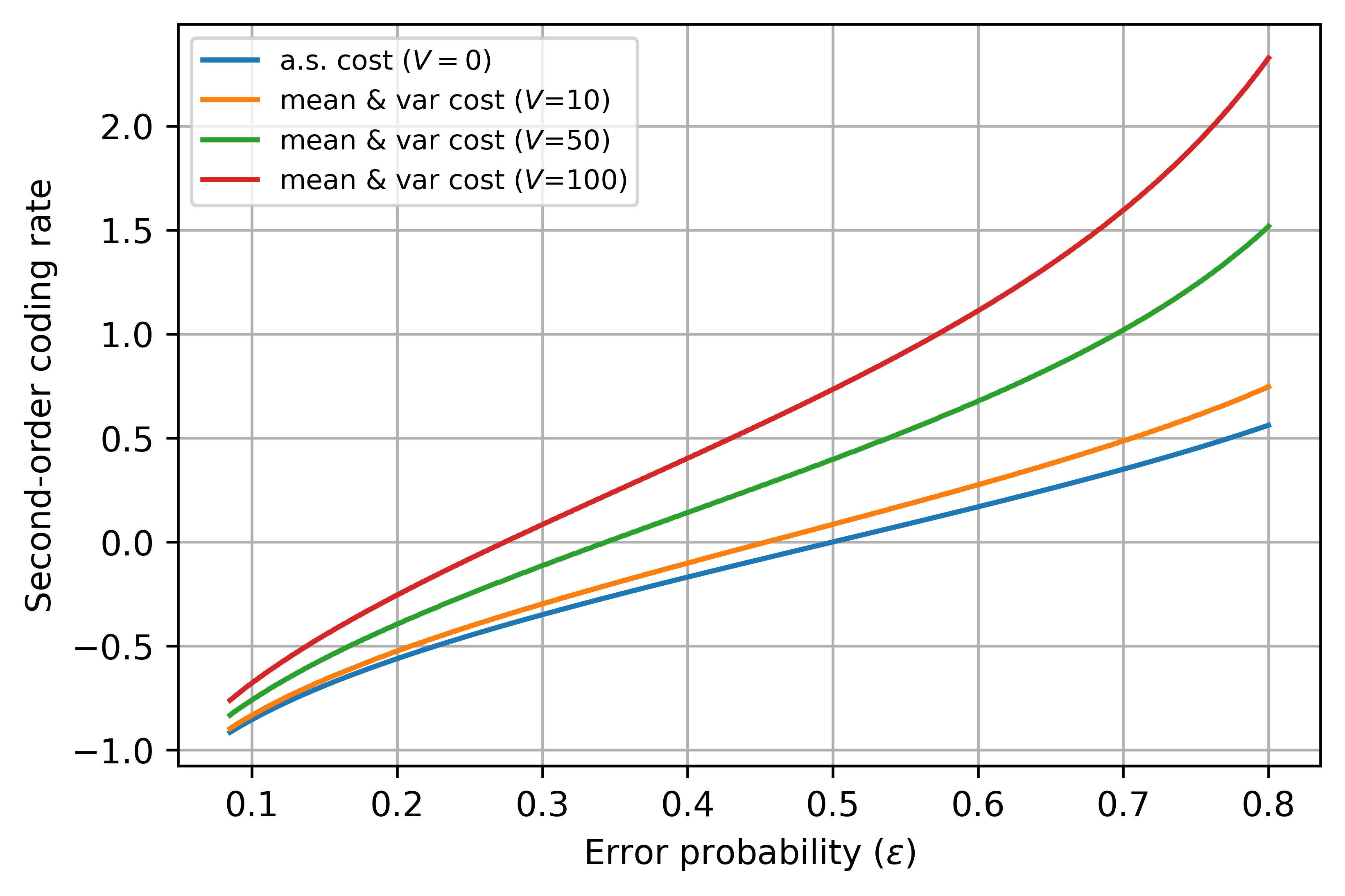
Let $r(\epsilon,\Gamma,V)$ denote the achievable SOCR for the mean and variance cost constraint in Theorem 1, which is also the optimal SOCR as shown later in Theorem 2. As remarked earlier, $r(\epsilon,\Gamma,0)=\sqrt{V(\Gamma)}\Phi^{-1}(\epsilon)$ is the optimal SOCR for the maximal cost constraint. Fig. 1 plots the SOCR against the average error probability for a Gaussian channel with $\Gamma=2$ and $N=1$ , showing improved SOCR for several values of $V$ . In fact, [2, Theorem 1] shows that $r(\epsilon,\Gamma,V)>\sqrt{V(\Gamma)}\Phi^{-1}(\epsilon)$ for all $V>0$ .

Refer to caption — Figure 1: The SOCR is compared between the almost-sure cost constraint and the mean and variance cost constraints for different values of $V$ . The plots for the mean and variance cost constraints are technically lower bounds to the SOCR since they are obtained through a non-exhaustive search of the feasible region in the maximization and minimization in the formulation of $r(\epsilon,\Gamma,V)$ .

Proof:

In view of Lemma 3, consider any distribution $P_{\Pi}$ which achieves the minimum in

\mathcal{K}\left(\frac{r}{\sqrt{V(\Gamma)}},\frac{C^{\prime}(\Gamma)^{2}V}{V(\Gamma)}\right).

Let $\Pi\sim P_{\Pi}$ , where we write

\displaystyle P_{\Pi}(\pi)=\begin{cases}p_{1}&\pi=\pi_{1}\\ p_{2}&\pi=\pi_{2}\\ p_{3}&\pi=\pi_{3}.\end{cases}

Recall that $\mathbb{E}[\Pi]=\frac{r}{\sqrt{V(\Gamma)}}$ and $\text{Var}(\Pi)\leq\frac{C^{\prime}(\Gamma)^{2}V}{V(\Gamma)}$ . For each $j\in\{1,2,3\}$ , let

\displaystyle\Gamma_{j}=\Gamma-\frac{\sqrt{V(\Gamma)}}{C^{\prime}(\Gamma)\sqrt{n}}\pi_{j}+\frac{r}{C^{\prime}(\Gamma)\sqrt{n}}.

(13)

We assume sufficiently large $n$ so that $\Gamma_{j}>0$ for all $j\in\{1,2,3\}$ . Let $P^{*}_{j}$ be the capacity-cost-achieving input distribution for $C(\Gamma_{j})$ and $Q_{j}^{*}$ be the corresponding optimal output distribution. Thus, $P_{j}^{*}=\mathcal{N}(0,\Gamma_{j})$ and $Q_{j}^{*}=\mathcal{N}(0,\Gamma_{j}+N)$ . Let $Q^{cc}_{j}$ be the output distribution induced by the input distribution $\text{Unif}(S^{n-1}_{R_{j}})$ for $R_{j}=\sqrt{n\Gamma_{j}}$ .

Achievability Scheme: Let the random channel input $\mathbf{X}$ be such that with probability $p_{j}$ , $\mathbf{X}\sim\text{Unif}(S^{n-1}_{R_{j}})$ . Denoting the distribution of $\mathbf{X}$ by $P$ , we can write

\displaystyle P=\sum_{j=1}^{3}p_{j}\cdot\text{Unif}(S^{n-1}_{R_{j}}).

The output distribution of $\mathbf{Y}$ induced by $P\circ W$ is

\displaystyle PW(\mathbf{y})

\displaystyle=\sum_{j=1}^{3}p_{j}Q_{j}^{cc}(\mathbf{y}).

We define

\displaystyle\mathcal{E}_{n}:=(P\circ W)\left(\frac{1}{n}\log\frac{W(\mathbf{Y}|\mathbf{X})}{PW(\mathbf{Y})}\leq C(\Gamma)+\frac{r}{\sqrt{n}}\right)

and show that $\limsup_{n\to\infty}\mathcal{E}_{n}<\epsilon$ which, by Lemma 4, would show that the random coding scheme achieves a second-order coding rate of $r$ .

Analysis: We first write

\displaystyle\mathcal{E}_{n}

\displaystyle=\sum_{j=1}^{3}p_{j}\mathbb{P}_{\mathbf{X}\sim\text{Unif}(S^{n-1}_{R_{j}})}\left(\frac{1}{n}\log\frac{W(\mathbf{Y}|\mathbf{X})}{PW(\mathbf{Y})}\leq C(\Gamma)+\frac{r}{\sqrt{n}}\right).

(14)

To proceed further, we upper bound

	$\displaystyle\mathbb{P}_{\mathbf{X}\sim\text{Unif}(S^{n-1}_{R_{j}})}\left(\frac{1}{n}\log\frac{W(\mathbf{Y}\|\mathbf{X})}{PW(\mathbf{Y})}\leq C(\Gamma)+\frac{r}{\sqrt{n}}\right)$		(15)
	$\displaystyle=\int_{\mathbf{y}\in\mathbb{R}^{n}}d\mathbf{y}Q_{j}^{cc}(\mathbf{y})\mathbb{P}\left(\frac{1}{n}\log\frac{W(\mathbf{y}\|\mathbf{X})}{PW(\mathbf{y})}\leq C(\Gamma)+\frac{r}{\sqrt{n}}\Big{\|}\mathbf{Y}=\mathbf{y}\right)$
	$\displaystyle\leq\int_{\mathbf{y}\in\mathbb{R}^{n}}d\mathbf{y}Q_{j}^{cc}(\mathbf{y})\mathbb{P}\left(\frac{1}{n}\log\frac{W(\mathbf{y}\|\mathbf{X})}{Q_{i}^{cc}(\mathbf{y})}\leq C(\Gamma)+\frac{r}{\sqrt{n}}\Big{\|}\mathbf{Y}=\mathbf{y}\right),$

where $i\in\{1,2,3\}$ depends on $\mathbf{y}$ and is such that $Q_{i}^{cc}(\mathbf{y})$ assigns the highest probability to $\mathbf{y}$ . We continue the derivation as

	$\displaystyle\mathbb{P}_{\mathbf{X}\sim\text{Unif}(S^{n-1}_{R_{j}})}\left(\frac{1}{n}\log\frac{W(\mathbf{Y}\|\mathbf{X})}{PW(\mathbf{Y})}\leq C(\Gamma)+\frac{r}{\sqrt{n}}\right)$
	$\displaystyle\leq\int_{\mathbf{y}\in\mathbb{R}^{n}}d\mathbf{y}Q_{j}^{cc}(\mathbf{y})\mathbb{P}\left(\log\frac{W(\mathbf{y}\|\mathbf{X})}{Q_{i}^{cc}(\mathbf{y})}\leq nC(\Gamma)+r\sqrt{n}\Big{\|}\mathbf{Y}=\mathbf{y}\right)$
	$\displaystyle=\int_{\mathbf{y}\in\mathbb{R}^{n}}d\mathbf{y}Q_{j}^{cc}(\mathbf{y})\mathbb{P}\left(\log\frac{W(\mathbf{y}\|\mathbf{X})}{Q_{j}^{cc}(\mathbf{y})}\leq nC(\Gamma)+r\sqrt{n}+\log\frac{Q_{i}^{cc}(\mathbf{y})}{Q_{j}^{cc}(\mathbf{y})}\Big{\|}\mathbf{Y}=\mathbf{y}\right)$
	$\displaystyle\leq\int_{\mathbf{y}\in\mathbb{R}^{n}}d\mathbf{y}Q_{j}^{cc}(\mathbf{y})\mathbb{P}\left(\log\frac{W(\mathbf{y}\|\mathbf{X})}{Q_{j}^{cc}(\mathbf{y})}\leq nC(\Gamma)+r\sqrt{n}+\kappa_{1}\log n\Big{\|}\mathbf{Y}=\mathbf{y}\right)+\delta_{n}^{(j)}.$		(16)

In the last inequality above, we used Lemma 6. Specifically, in Lemma 6, let

•

$\Gamma=\Gamma_{j}$ ,
•

$\Gamma^{\prime}=\Gamma_{i}$ ,
•

$\epsilon=\Gamma_{i}-\Gamma_{j}$ so that $\epsilon=O\left(\frac{1}{\sqrt{n}}\right)$ , and
•

$\Delta=\sqrt{\frac{\log n}{n}}$ .

Consequently, $\kappa_{1}$ is a constant from the result of Lemma 6 and

\displaystyle\delta_{n}^{(j)}=Q_{j}^{cc}\left(\Bigg{|}\frac{||\mathbf{Y}||^{2}}{n}-\Gamma_{j}-N\Bigg{|}>\Delta\right).

It is easy to check that for $\mathbf{Y}\sim Q_{j}^{cc}$ , $\mathbb{E}\left[||\mathbf{Y}||^{2}\right]=n\Gamma_{j}+nN$ and $\text{Var}(||\mathbf{Y}||^{2})=4nN\Gamma_{j}+2nN^{2}$ . Thus, it is easy to see that $\delta_{n}^{(j)}\to 0$ as $n\to\infty$ using Chebyshev inequality.

Continuing the derivation from $(\ref{1zp})$ , we have

	$\displaystyle\mathbb{P}_{\mathbf{X}\sim\text{Unif}(S^{n-1}_{R_{j}})}\left(\frac{1}{n}\log\frac{W(\mathbf{Y}\|\mathbf{X})}{PW(\mathbf{Y})}\leq C(\Gamma)+\frac{r}{\sqrt{n}}\right)$
	$\displaystyle\leq\int_{\mathbf{y}\in\mathbb{R}^{n}}d\mathbf{y}Q_{j}^{cc}(\mathbf{y})\mathbb{P}\left(\log\frac{W(\mathbf{y}\|\mathbf{X})}{Q_{j}^{}(\mathbf{y})}\leq nC(\Gamma)+r\sqrt{n}+\kappa_{1}\log n+\log\frac{Q_{j}^{cc}(\mathbf{y})}{Q_{j}^{}(\mathbf{y})}\Big{\|}\mathbf{Y}=\mathbf{y}\right)+\delta_{n}^{(j)}$
	$\displaystyle\leq\int_{\mathbf{y}\in\mathbb{R}^{n}}d\mathbf{y}Q_{j}^{cc}(\mathbf{y})\mathbb{P}\left(\log\frac{W(\mathbf{y}\|\mathbf{X})}{Q_{j}^{*}(\mathbf{y})}\leq nC(\Gamma)+r\sqrt{n}+\kappa\log n\Big{\|}\mathbf{Y}=\mathbf{y}\right)+2\delta_{n}^{(j)}.$		(17)

In the last inequality above, we used Lemma 7. Specifically, in Lemma 7, let $\Gamma=\Gamma_{j}$ and $\Delta=\sqrt{\frac{\log n}{n}}$ . Consequently, $\kappa$ is a suitable bounding constant for both Lemma 6 and Lemma 7.

Continuing the derivation from $(\ref{2x})$ , we have

	$\displaystyle\mathbb{P}_{\mathbf{X}\sim\text{Unif}(S^{n-1}_{R_{j}})}\left(\frac{1}{n}\log\frac{W(\mathbf{Y}\|\mathbf{X})}{PW(\mathbf{Y})}\leq C(\Gamma)+\frac{r}{\sqrt{n}}\right)$
	$\displaystyle\leq\mathbb{P}_{\mathbf{X}\sim\text{Unif}(S^{n-1}_{R_{j}})}\left(\log\frac{W(\mathbf{Y}\|\mathbf{X})}{Q_{j}^{*}(\mathbf{Y})}\leq nC(\Gamma)+r\sqrt{n}+\kappa\log n\right)+2\delta_{n}^{(j)}$
	$\displaystyle=\mathbb{P}_{\mathbf{X}\sim\text{Unif}(S^{n-1}_{R_{j}})}\left(\sum_{m=1}^{n}\log\frac{W(Y_{m}\|X_{m})}{Q_{j}^{*}(Y_{m})}-nC(\Gamma_{j})\leq n\left(C(\Gamma)-C(\Gamma_{j})\right)+r\sqrt{n}+\kappa\log n\right)+2\delta_{n}^{(j)}$
	$\displaystyle\stackrel{{\scriptstyle(a)}}{{=}}\mathbb{P}_{\mathbf{X}\sim\text{Unif}(S^{n-1}_{R_{j}})}\left(\sum_{m=1}^{n}\left[\log\frac{W(Y_{m}\|X_{m})}{Q_{j}^{}(Y_{m})}-\mathbb{E}\left[\log\frac{W(Y_{m}\|X_{m})}{Q_{j}^{}(Y_{m})}\right]\right]\leq n\left(C(\Gamma)-C(\Gamma_{j})\right)+r\sqrt{n}+\kappa\log n\right)+2\delta_{n}^{(j)}$
	$\displaystyle\stackrel{{\scriptstyle(b)}}{{=}}\mathbb{P}\left(\sum_{m=1}^{n}\tilde{T}_{m}\leq n\left(C(\Gamma)-C(\Gamma_{j})\right)+r\sqrt{n}+\kappa\log n\right)+2\delta_{n}^{(j)}$
	$\displaystyle\stackrel{{\scriptstyle(c)}}{{=}}\mathbb{P}\left(\frac{1}{\sqrt{nV(\Gamma_{j})}}\sum_{m=1}^{n}\tilde{T}_{m}\leq\sqrt{n}\frac{C(\Gamma)-C(\Gamma_{j})}{\sqrt{V(\Gamma_{j})}}+\frac{r}{\sqrt{V(\Gamma_{j})}}+\frac{\kappa\log n}{\sqrt{nV(\Gamma_{j})}}\right)+2\delta_{n}^{(j)}$

	$\displaystyle\stackrel{{\scriptstyle(d)}}{{\leq}}\Phi\left(\sqrt{n}\frac{C(\Gamma)-C(\Gamma_{j})}{\sqrt{V(\Gamma_{j})}}+\frac{r}{\sqrt{V(\Gamma_{j})}}+\frac{\kappa\log n}{\sqrt{nV(\Gamma_{j})}}\right)+\delta_{n}$
	$\displaystyle\stackrel{{\scriptstyle(e)}}{{\leq}}\Phi\left(\frac{\sqrt{n}}{2\sqrt{V(\Gamma_{j})}}\left(\frac{\Gamma-\Gamma_{j}}{N+\Gamma}\right)+\frac{r}{\sqrt{V(\Gamma_{j})}}+\frac{2\kappa\log n}{\sqrt{nV(\Gamma_{j})}}\right)+\delta_{n}$		(18)

In equality $(a)$ above, we used Lemma 1. Specifically, use Equation $(\ref{equsentimes})$ in Lemma 1 with $\Gamma=\Gamma_{j}$ .

In equality $(b)$ above, we used Lemma 2, where the $\tilde{T}_{m}$ ’s are i.i.d. and

\displaystyle\tilde{T}_{m}=\log\frac{W(Y|\sqrt{\Gamma_{j}})}{Q^{*}_{j}(Y)}-\mathbb{E}\left[\log\frac{W(Y|\sqrt{\Gamma_{j}})}{Q^{*}_{j}(Y)}\right],

(19)

where $Y\sim\mathcal{N}(\sqrt{\Gamma_{j}},N)$ .

In equality $(c)$ above, we normalize the sum to have unit variance, which follows from Corollary 1 and Equation $(\ref{VGammadef})$ .

In inequality $(d)$ above, we used the Berry-Esseen Theorem [12] to obtain convergence of the CDF of the normalized sum of i.i.d. random variables $\tilde{T}_{m}$ ’s to the standard normal CDF, with $\delta_{n}\to 0$ accounting for both the rate of convergence and $\delta_{n}^{(j)}\to 0$ . In inequality $(e)$ above, we used a Taylor series approximation, noting that $\Gamma-\Gamma_{j}=O(1/\sqrt{n})$ .

Substituting $(\ref{subsintosumof3})$ into $(\ref{epsnu})$ , we obtain

\displaystyle\mathcal{E}_{n}

\displaystyle\leq\sum_{j=1}^{3}p_{j}\Phi\left(\frac{\sqrt{n}}{2\sqrt{V(\Gamma_{j})}}\left(\frac{\Gamma-\Gamma_{j}}{N+\Gamma}\right)+\frac{r}{\sqrt{V(\Gamma_{j})}}+\frac{2\kappa\log n}{\sqrt{nV(\Gamma_{j})}}\right)+\delta_{n}

for some redefined sequence $\delta_{n}\to 0$ as $n\to\infty$ . Using Equation $(\ref{38n})$ and the formula for $C^{\prime}(\Gamma)$ from Lemma 1, we can simplify the upper bound as

\displaystyle\mathcal{E}_{n}

\displaystyle\leq\sum_{j=1}^{3}p_{j}\Phi\left(\frac{\sqrt{V(\Gamma)}}{\sqrt{V(\Gamma_{j})}}\pi_{j}-\frac{r}{\sqrt{V(\Gamma_{j})}}+\frac{r}{\sqrt{V(\Gamma_{j})}}+\frac{2\kappa\log n}{\sqrt{nV(\Gamma_{j})}}\right)+\delta_{n}.

Therefore, since $\Gamma_{j}\to\Gamma$ as $n\to\infty$ , we have

	$\displaystyle\limsup_{n\to\infty}\mathcal{E}_{n}$	$\displaystyle\leq\sum_{j=1}^{3}p_{j}\Phi\left(\pi_{j}\right)$
		$\displaystyle=\mathcal{K}\left(\frac{r}{\sqrt{V(\Gamma)}},\frac{C^{\prime}(\Gamma)^{2}V}{V(\Gamma)}\right).$		(20)

To complete the proof, we choose $r<r^{*}$ where

\displaystyle r^{*}=\max\left\{r:\mathcal{K}\left(\frac{r}{\sqrt{V(\Gamma)}},\frac{C^{\prime}(\Gamma)^{2}V}{V(\Gamma)}\right)\leq\epsilon\right\}.

(21)

Hence, $\limsup_{n\to\infty}\mathcal{E}_{n}<\epsilon$ because, from Lemma 3, $\mathcal{K}(\cdot,\cdot)$ is a strictly increasing function in the first argument. Hence, $\limsup_{n\to\infty}\mathcal{E}_{n}<\epsilon$ for $r<r^{*}$ , thus establishing that any $r<r^{*}$ is an achievable second-order coding rate. Finally, letting $r\to r^{*}$ establishes an achievable second-order coding rate of $r^{*}$ , matching the converse in Theorem 2.

The achievability result can also be stated in terms of an upper bound on the minimum average probability of error of $(n,R,\Gamma,V)$ codes for a rate $R=C(\Gamma)+\frac{r}{\sqrt{n}}$ . From Lemma 4, we have for $\theta=1/n^{\vartheta}$ for $1>\vartheta>1/2$ ,

\displaystyle\bar{P}_{\text{e}}\left(n,C(\Gamma)+\frac{r}{\sqrt{n}},\Gamma,V\right)\leq(P\circ W)\left(\frac{1}{n}\log\frac{W(\mathbf{Y}|\mathbf{X})}{PW(\mathbf{Y})}\leq C(\Gamma)+\frac{r}{\sqrt{n}}+\frac{1}{n^{\vartheta}}\right)+e^{-n^{1-\vartheta}}.

(22)

For any $r^{\prime}>r$ , we have $\frac{r}{\sqrt{n}}+\frac{1}{n^{\vartheta}}<\frac{r^{\prime}}{\sqrt{n}}$ eventually, so

	$\displaystyle\limsup_{n\to\infty}\bar{P}_{\text{e}}\left(n,C(\Gamma)+\frac{r}{\sqrt{n}},\Gamma,V\right)$
	$\displaystyle\leq\limsup_{n\to\infty}(P\circ W)\left(\frac{1}{n}\log\frac{W(\mathbf{Y}\|\mathbf{X})}{PW(\mathbf{Y})}\leq C(\Gamma)+\frac{r^{\prime}}{\sqrt{n}}\right)$
	$\displaystyle\leq\mathcal{K}\left(\frac{r^{\prime}}{\sqrt{V(\Gamma)}},\frac{C^{\prime}(\Gamma)^{2}V}{V(\Gamma)}\right),$		(23)

where the last inequality follows from $(\ref{extendtoerror})$ . Letting $r^{\prime}\to r$ in $(\ref{notplayggg})$ and invoking continuity of the function $\mathcal{K}$ establishes the result.

∎

IV Converse Result

Lemma 8

Consider an AWGN channel $W$ with noise variance $N>0$ and cost constraint $(\Gamma,V)\in(0,\infty)\times(0,\infty)$ . Then for every $n,\rho>0$ and $\epsilon\in(0,1)$ ,

\displaystyle\log M^{*}(n,\epsilon,\Gamma,V)

\displaystyle\leq\log\rho-\log\left[\left(1-\epsilon-\sup_{\overline{P}\in\mathcal{P}_{\Gamma,V}(\mathbb{R}^{n})}\,\inf_{q\in\mathcal{P}(\mathbb{R}^{n})}(\overline{P}\circ W)\left(\frac{W(\mathbf{Y}|\mathbf{X})}{q(\mathbf{Y})}>\rho\right)\right)^{+}\right],

(24)

where $\mathcal{P}_{\Gamma,V}(\mathbb{R}^{n})\subset\mathcal{P}(\mathbb{R}^{n})$ is the set of distributions $\overline{P}$ such that $\mathbb{E}\left[\sum_{i=1}^{n}c(X_{i})\right]\leq n\Gamma$ and $\text{Var}\left(\sum_{i=1}^{n}c(X_{i})\right)\leq nV$ for $\mathbf{X}\sim\overline{P}$ .

Proof: The proof is similar to that of [9, Lemma 2] and is omitted.

Theorem 2

Fix an arbitrary $\epsilon\in(0,1)$ . Consider an AWGN channel with noise variance $N>0$ . Under the mean and variance cost constraints specified by the pair $(\Gamma,V)\in(0,\infty)\times[0,\infty)$ , we have

\displaystyle\limsup_{n\to\infty}\,\frac{\log M^{*}(n,\epsilon,\Gamma,V)-nC(\Gamma)}{\sqrt{n}}\leq\max\left\{r\in\mathbb{R}:\mathcal{K}\left(\frac{r}{\sqrt{V(\Gamma)}},\frac{C^{\prime}(\Gamma)^{2}V}{V(\Gamma)}\right)\leq\epsilon\right\}.

(25)

Alternatively, for any second-order coding rate $r\in\mathbb{R}$ ,

\displaystyle\liminf_{n\to\infty}\bar{P}_{\text{e}}\left(n,C(\Gamma)+\frac{r}{\sqrt{n}},\Gamma,V\right)

\displaystyle\geq\mathcal{K}\left(\frac{r}{\sqrt{V(\Gamma)}},\frac{C^{\prime}(\Gamma)^{2}V}{V(\Gamma)}\right).

(26)

Proof:

For $V=0$ , we are required to prove that the upper bound in $(\ref{upper_bound_V=0})$ is $\sqrt{V(\Gamma)}\Phi^{-1}(\epsilon)$ , and the lower bound in $(\ref{lower_bound_V=0})$ is $\Phi\left(r/\sqrt{V(\Gamma)}\right)$ . But this follows from the known converse results for the maximal cost constraint, since the m.v. cost constraint for $V=0$ is more stringent.

We assume $V>0$ for the remainder of the proof. We start with Lemma 8 and first upper bound

\displaystyle\sup_{\overline{P}\in\mathcal{P}_{\Gamma,V}(\mathbb{R}^{n})}\,\inf_{q\in\mathcal{P}(\mathbb{R}^{n})}(\overline{P}\circ W)\left(\frac{W(\mathbf{Y}|\mathbf{X})}{q(\mathbf{Y})}>\rho\right).

(27)

Let $\rho=\exp\left(nC(\Gamma)+\sqrt{n}r\right)$ in $(\ref{bx})$ , where $r$ is a number to be specified later. Let $\mathbf{X}\sim\overline{P}$ for any arbitrary $\overline{P}\in\mathcal{P}_{\Gamma,V}(\mathbb{R}^{n})$ so that $\mathbb{E}\left[\sum_{i=1}^{n}c(X_{i})\right]\leq n\Gamma$ and $\text{Var}\left(\sum_{i=1}^{n}c(X_{i})\right)\leq nV$ .

Choosing $q=Q^{*}$ in $(\ref{bx})$ , we have

	$\displaystyle(\overline{P}\circ W)\left(\log\frac{W(\mathbf{Y}\|\mathbf{X})}{Q^{*}(\mathbf{Y})}>nC(\Gamma)+\sqrt{n}r\right)$
	$\displaystyle=\int_{\mathbb{R}^{n}}d\overline{P}(\mathbf{x})W\left(\sum_{i=1}^{n}\log\frac{W(Y_{i}\|x_{i})}{Q^{*}(Y_{i})}>nC(\Gamma)+\sqrt{n}r\right),$		(28)

where in $(\ref{fopv})$ , $Y_{1},Y_{2},\ldots,Y_{n}$ are independent random variables and each $Y_{i}\sim\mathcal{N}(x_{i},N)$ . We define the empirical distribution of a vector $\mathbf{x}$ as

\displaystyle P_{\mathbf{x}}=\frac{1}{n}\sum_{i=1}^{n}\delta_{x_{i}},

where $\delta_{x}$ is the dirac delta measure at $x$ . For any given channel input $\mathbf{x}$ and independent $Y_{i}$ ’s where $Y_{i}\sim\mathcal{N}(x_{i},N)$ , we have from Corollary 1 that

	$\displaystyle\text{Var}\left(\frac{1}{\sqrt{n}}\sum_{i=1}^{n}\left[\log\frac{W(Y_{i}\|x_{i})}{Q^{}(Y_{i})}-\mathbb{E}\left[\log\frac{W(Y_{i}\|x_{i})}{Q^{}(Y_{i})}\right]\right]\right)$
	$\displaystyle=\int\nu_{t}P_{\mathbf{x}}(t)dt$
	$\displaystyle=\frac{\Gamma^{2}+2Nc(\mathbf{x})}{2(N+\Gamma)^{2}}$

For any $\beta\geq 0$ , define

\displaystyle\delta_{\beta}:=\sup_{\Gamma-\beta<t\leq\Gamma+\beta}\Bigg{|}\frac{\Gamma^{2}+2Nt}{2(N+\Gamma)^{2}}-V(\Gamma)\Bigg{|}

and note that $\delta_{\beta}\to 0$ as $\beta\to 0$ . Define the function

\displaystyle\psi_{\beta}\left(t\right):=\begin{cases}V(\Gamma)+\delta_{\beta}&\text{ if }t\leq\Gamma\\ V(\Gamma)-\delta_{\beta}&\text{ if }t>\Gamma.\end{cases}

Fix any $0<\Delta<1/2$ and $\eta>0$ . Then select $\beta>0$ such that $\delta_{\beta}<V(\Gamma)$ ,

\displaystyle\sup_{t\in\mathbb{R}}\Bigg{|}\frac{1}{\sqrt{V(\Gamma)}}-\frac{1}{\sqrt{\psi_{\beta}(t)}}\Bigg{|}\leq\frac{\Delta}{C^{\prime}(\Gamma)\sqrt{V}}

(29)

and

\displaystyle\sup_{t\in\mathbb{R}}\Bigg{|}\frac{1}{V(\Gamma)}-\frac{1}{\psi_{\beta}(t)}\Bigg{|}\leq\frac{\Delta/2}{C^{\prime}(\Gamma)^{2}V}.

(30)

Also define

\displaystyle\varphi(r):=\begin{cases}V(\Gamma)-\delta_{\beta}&\text{ if }r\leq 0\\ V(\Gamma)+\delta_{\beta}&\text{ if }r>0.\end{cases}

(31)

With $\Delta$ , $\eta$ and $\beta$ fixed as above¹¹1 $\eta$ is used later., we divide the set of sequences $\mathbf{x}\in\mathbb{R}^{n}$ into three subsets:

	$\displaystyle\mathcal{P}_{n,1}$	$\displaystyle:=\left\{\mathbf{x}:c(\mathbf{x})\leq\Gamma-\beta\right\},$
	$\displaystyle\mathcal{P}_{n,2}$	$\displaystyle:=\left\{\mathbf{x}:\Gamma-\beta<c(\mathbf{x})\leq\Gamma+\beta\right\},$
	$\displaystyle\mathcal{P}_{n,3}$	$\displaystyle:=\left\{\mathbf{x}:c(\mathbf{x})>\Gamma+\beta\right\}.$

For $\mathbf{x}\in\mathcal{P}_{n,1}$ , we have

	$\displaystyle W\left(\sum_{i=1}^{n}\log\frac{W(Y_{i}\|x_{i})}{Q^{*}(Y_{i})}>nC(\Gamma)+\sqrt{n}r\right)$
	$\displaystyle\stackrel{{\scriptstyle(a)}}{{=}}W\left(\sum_{i=1}^{n}\left[\log\frac{W(Y_{i}\|x_{i})}{Q^{}(Y_{i})}-\mathbb{E}\left[\log\frac{W(Y_{i}\|x_{i})}{Q^{}(Y_{i})}\right]\right]>nC^{\prime}(\Gamma)\left(\Gamma-c(\mathbf{x})\right)+\sqrt{n}r\right)$
	$\displaystyle\leq W\left(\sum_{i=1}^{n}\left[\log\frac{W(Y_{i}\|x_{i})}{Q^{}(Y_{i})}-\mathbb{E}\left[\log\frac{W(Y_{i}\|x_{i})}{Q^{}(Y_{i})}\right]\right]>nC^{\prime}(\Gamma)\beta+\sqrt{n}r\right)$
	$\displaystyle\stackrel{{\scriptstyle(b)}}{{\leq}}W\left(\sum_{i=1}^{n}\left[\log\frac{W(Y_{i}\|x_{i})}{Q^{}(Y_{i})}-\mathbb{E}\left[\log\frac{W(Y_{i}\|x_{i})}{Q^{}(Y_{i})}\right]\right]>\frac{nC^{\prime}(\Gamma)\beta}{2}\right)$
	$\displaystyle\stackrel{{\scriptstyle(c)}}{{\leq}}\frac{4}{nC^{\prime}(\Gamma)^{2}\beta^{2}}\left(\frac{\Gamma^{2}+2N\Gamma}{2(N+\Gamma)^{2}}\right)$		(32)

for sufficiently large $n$ . In equality $(a)$ , we used Lemma 1. Inequality $(b)$ holds because $r$ is a constant. Inequality $(c)$ follows by applying Chebyshev’s inequality and Corollary 1, the latter of which gives us that

	$\displaystyle\text{Var}\left(\sum_{i=1}^{n}\left[\log\frac{W(Y_{i}\|x_{i})}{Q^{}(Y_{i})}-\mathbb{E}\left[\log\frac{W(Y_{i}\|x_{i})}{Q^{}(Y_{i})}\right]\right]\right)$
	$\displaystyle=\frac{n\Gamma^{2}+2nNc(\mathbf{x})}{2\left(N+\Gamma\right)^{2}}$
	$\displaystyle\leq n\left(\frac{\Gamma^{2}+2N\Gamma}{2(N+\Gamma)^{2}}\right).$

For $\mathbf{x}\in\mathcal{P}_{n,2}$ , we have

	$\displaystyle W\left(\sum_{i=1}^{n}\log\frac{W(Y_{i}\|x_{i})}{Q^{*}(Y_{i})}>nC(\Gamma)+\sqrt{n}r\right)$
	$\displaystyle\stackrel{{\scriptstyle(a)}}{{=}}W\left(\sum_{i=1}^{n}\left[\log\frac{W(Y_{i}\|x_{i})}{Q^{}(Y_{i})}-\mathbb{E}\left[\log\frac{W(Y_{i}\|x_{i})}{Q^{}(Y_{i})}\right]\right]>nC^{\prime}(\Gamma)\left(\Gamma-c(\mathbf{x})\right)+\sqrt{n}r\right)$
	$\displaystyle\stackrel{{\scriptstyle(b)}}{{=}}W\left(\frac{1}{\sqrt{\int n\,\nu_{t}P_{\mathbf{x}}(t)dt}}\sum_{i=1}^{n}\left[\log\frac{W(Y_{i}\|x_{i})}{Q^{}(Y_{i})}-\mathbb{E}\left[\log\frac{W(Y_{i}\|x_{i})}{Q^{}(Y_{i})}\right]\right]>\mbox{}\right.$
	$\displaystyle\left.\quad\quad\quad\quad\quad\quad\quad\quad\quad\frac{\sqrt{n}C^{\prime}(\Gamma)\left(\Gamma-c(\mathbf{x})\right)}{\sqrt{\int\nu_{t}P_{\mathbf{x}}(t)dt}}+\frac{r}{\sqrt{\int\nu_{t}P_{\mathbf{x}}(t)dt}}\right)$
	$\displaystyle\stackrel{{\scriptstyle(c)}}{{=}}W\left(\frac{1}{\sqrt{\int n\,\nu_{t}P_{\mathbf{x}}(t)dt}}\sum_{i=1}^{n}\tilde{T}_{i}>\frac{\sqrt{n}C^{\prime}(\Gamma)\left(\Gamma-c(\mathbf{x})\right)}{\sqrt{\int\nu_{t}P_{\mathbf{x}}(t)dt}}+\frac{r}{\sqrt{\int\nu_{t}P_{\mathbf{x}}(t)dt}}\right)$
	$\displaystyle\stackrel{{\scriptstyle(d)}}{{\leq}}1-\Phi\left(\frac{\sqrt{n}C^{\prime}(\Gamma)\left(\Gamma-c(\mathbf{x})\right)}{\sqrt{\int\nu_{t}P_{\mathbf{x}}(t)dt}}+\frac{r}{\sqrt{\int\nu_{t}P_{\mathbf{x}}(t)dt}}\right)+\frac{\kappa_{\mathbf{x}}}{\sqrt{n}}$
	$\displaystyle\stackrel{{\scriptstyle(e)}}{{\leq}}1-\Phi\left(\frac{\sqrt{n}C^{\prime}(\Gamma)\left(\Gamma-c(\mathbf{x})\right)}{\sqrt{\int\nu_{t}P_{\mathbf{x}}(t)dt}}+\frac{r}{\sqrt{\int\nu_{t}P_{\mathbf{x}}(t)dt}}\right)+\frac{\kappa}{\sqrt{n}}$
	$\displaystyle\leq 1-\Phi\left(\frac{\sqrt{n}C^{\prime}(\Gamma)\left(\Gamma-c(\mathbf{x})\right)}{\sqrt{\psi_{\beta}(c(\mathbf{x}))}}+\frac{r}{\sqrt{\varphi(r)}}\right)+\frac{\kappa}{\sqrt{n}}$		(33)

for sufficiently large $n$ . In equality $(a)$ , we used Lemma 1. In equality $(b)$ , we normalize the sum to have unit variance, where we write

	$\displaystyle\int_{-\infty}^{\infty}n\,\nu_{t}P_{\mathbf{x}}(t)dt$
	$\displaystyle=\text{Var}\left(\sum_{i=1}^{n}\left[\log\frac{W(Y_{i}\|x_{i})}{Q^{}(Y_{i})}-\mathbb{E}\left[\log\frac{W(Y_{i}\|x_{i})}{Q^{}(Y_{i})}\right]\right]\right)$
	$\displaystyle=\frac{n\Gamma^{2}+2nNc(\mathbf{x})}{2\left(N+\Gamma\right)^{2}}.$

In equality $(c)$ , we use Lemma 2. In inequality $(d)$ , we apply the Berry-Esseen Theorem [12], where $\kappa_{\mathbf{x}}$ is a constant depending on the second- and third-order moments of $\{\tilde{T}_{i}\}_{i=1}^{n}$ . In inequality $(e)$ , we use the fact that the distribution of each $\tilde{T}_{i}$ depends on $\mathbf{x}$ only through its cost $c(\mathbf{x})$ . Since $c(\mathbf{x})$ is uniformly bounded over the set $\mathcal{P}_{n,2}$ , the constant $\kappa_{\mathbf{x}}$ can be uniformly upper bounded over all $\mathbf{x}\in\mathcal{P}_{n,2}$ by some constant $\kappa$ that does not depend on $\mathbf{x}$ at all.

For $\mathcal{P}_{n,3}$ , the following lemma shows that the probability of this set under $\overline{P}$ is small.

Lemma 9

We have

\displaystyle\overline{P}\left(\mathcal{P}_{n,3}\right)\leq\frac{V}{n\beta^{2}}.

(34)

Proof:

Let $\mu_{i}=\mathbb{E}[c(X_{i})]$ . For any $\beta>0$ ,

	$\displaystyle\overline{P}\left(c(\mathbf{X})>\Gamma+\beta\right)$
	$\displaystyle=\overline{P}\left(\sum_{i=1}^{n}\left(c(X_{i})-\mu_{i}\right)+\sum_{i=1}^{n}\mu_{i}\geq n\Gamma+n\beta\right)$
	$\displaystyle\leq\overline{P}\left(\sum_{i=1}^{n}\left(c(X_{i})-\mu_{i}\right)\geq n\beta\right)$
	$\displaystyle\leq\overline{P}\left(\left(\sum_{i=1}^{n}\left(c(X_{i})-\mu_{i}\right)\right)^{2}\geq n^{2}\beta^{2}\right)$
	$\displaystyle\leq\frac{1}{n^{2}\beta^{2}}\mathbb{E}\left[\left(\sum_{i=1}^{n}\left(c(X_{i})-\mu_{i}\right)\right)^{2}\right]$
	$\displaystyle\leq\frac{V}{n\beta^{2}}.$

∎

Using the results in $(\ref{pn1})$ , $(\ref{pn2})$ and $(\ref{pn3})$ , we can upper bound $(\ref{fopv})$ as

	$\displaystyle(\overline{P}\circ W)\left(\log\frac{W(\mathbf{Y}\|\mathbf{X})}{Q^{*}(\mathbf{Y})}>nC(\Gamma)+\sqrt{n}r\right)$
	$\displaystyle\leq 1+\frac{4}{nC^{\prime}(\Gamma)^{2}\beta^{2}}\left(\frac{\Gamma^{2}+2N\Gamma}{2(N+\Gamma)^{2}}\right)+\frac{V}{n\beta^{2}}+\frac{\kappa}{\sqrt{n}}-\mbox{}$
	$\displaystyle\quad\quad\quad\mathbb{E}\left[\Phi\left(\frac{\sqrt{n}C^{\prime}(\Gamma)\left(\Gamma-c(\mathbf{X})\right)}{\sqrt{\psi_{\beta}(c(\mathbf{X}))}}+\frac{r}{\sqrt{\varphi(r)}}\right)\right].$		(35)

To further upper bound the above expression, we need to obtain a lower bound to

\displaystyle\inf_{\mathbf{X}}\,\mathbb{E}\left[\Phi\left(\frac{\sqrt{n}C^{\prime}(\Gamma)\left(\Gamma-c(\mathbf{X})\right)}{\sqrt{\psi_{\beta}(c(\mathbf{X}))}}+\frac{r}{\sqrt{\varphi(r)}}\right)\right],

where the infimum is over all random vectors $\mathbf{X}$ such that $\mathbb{E}\left[c(\mathbf{X})\right]\leq\Gamma$ and $\text{Var}\left(c(\mathbf{X})\right)\leq V/n$ . Without loss of generality, we can assume $\mathbb{E}[c(\mathbf{X})]=\Gamma$ since the function $\Phi$ is monotonically increasing and the function

c\mapsto\frac{\Gamma-c}{\sqrt{\psi_{\beta}(c)}}

is monotonically nonincreasing.

Note that

	$\displaystyle\Bigg{\|}\mathbb{E}\left[\frac{\sqrt{n}C^{\prime}(\Gamma)}{\sqrt{\psi_{\beta}(c(\mathbf{X}))}}\left(\Gamma-c(\mathbf{X})\right)\right]-\mathbb{E}\left[\frac{\sqrt{n}C^{\prime}(\Gamma)}{\sqrt{V(\Gamma)}}\left(\Gamma-c(\mathbf{X})\right)\right]\Bigg{\|}$
	$\displaystyle=\Bigg{\|}\mathbb{E}\left[\sqrt{n}C^{\prime}(\Gamma)\left(\Gamma-c(\mathbf{X})\right)\left[\frac{1}{\sqrt{\psi_{\beta}(c(\mathbf{X}))}}-\frac{1}{\sqrt{V(\Gamma)}}\right]\right]\Bigg{\|}$
	$\displaystyle\leq\sqrt{n}C^{\prime}(\Gamma)\mathbb{E}\left[\big{\|}\Gamma-c(\mathbf{X})\big{\|}\cdot\Bigg{\|}\frac{1}{\sqrt{\psi_{\beta}(c(\mathbf{X}))}}-\frac{1}{\sqrt{V(\Gamma)}}\Bigg{\|}\right]$
	$\displaystyle\stackrel{{\scriptstyle(a)}}{{\leq}}\sqrt{n}C^{\prime}(\Gamma)\frac{\Delta}{C^{\prime}(\Gamma)\sqrt{V}}\mathbb{E}\left[\big{\|}\Gamma-c(\mathbf{X})\big{\|}\right]$
	$\displaystyle\stackrel{{\scriptstyle(b)}}{{\leq}}\Delta.$		(36)

In inequality $(a)$ , we used $(\ref{aaronerr1})$ . In inequality $(b)$ , we used the fact that $\mathbb{E}\left[\sqrt{\left(\Gamma-c(\mathbf{X})\right)^{2}}\right]\leq\sqrt{\text{Var}(c(\mathbf{X}))}$ . Hence, from $(\ref{bzuyv})$ , we have

	$\displaystyle\mathbb{E}\left[\frac{\sqrt{n}C^{\prime}(\Gamma)}{\sqrt{\psi_{\beta}(c(\mathbf{X}))}}\left(\Gamma-c(\mathbf{X})\right)\right]$
	$\displaystyle\geq\mathbb{E}\left[\frac{\sqrt{n}C^{\prime}(\Gamma)}{\sqrt{V(\Gamma)}}\left(\Gamma-c(\mathbf{X})\right)\right]-\Delta$
	$\displaystyle=-\Delta.$		(37)

Now define $X^{\prime}=\Gamma-c(\mathbf{X})$ so that $\mathbb{E}[X^{\prime}]=0$ and $\text{Var}(X^{\prime})\leq V/n$ . Also define

\displaystyle\Psi_{\beta}(X^{\prime}):=\begin{cases}V(\Gamma)+\delta_{\beta}&\text{ if }X^{\prime}\geq 0\\ V(\Gamma)-\delta_{\beta}&\text{ if }X^{\prime}<0.\end{cases}

Then note that

	$\displaystyle\Bigg{\|}\text{Var}\left(\frac{\Gamma-c(\mathbf{X})}{\sqrt{\psi_{\beta}(c(\mathbf{X}))}}\right)-\text{Var}\left(\frac{\Gamma-c(\mathbf{X})}{\sqrt{V(\Gamma)}}\right)\Bigg{\|}$
	$\displaystyle=\Bigg{\|}\text{Var}\left(\frac{X^{\prime}}{\sqrt{\Psi_{\beta}(X^{\prime})}}\right)-\text{Var}\left(\frac{X^{\prime}}{\sqrt{V(\Gamma)}}\right)\Bigg{\|}$
	$\displaystyle=\Bigg{\|}\mathbb{E}\left[\frac{X^{\prime 2}}{\Psi_{\beta}(X^{\prime})}-\frac{X^{\prime 2}}{V(\Gamma)}\right]+\left(\mathbb{E}\left[\frac{X^{\prime}}{\sqrt{V(\Gamma)}}\right]\right)^{2}-\left(\mathbb{E}\left[\frac{X^{\prime}}{\sqrt{\Psi_{\beta}(X^{\prime})}}\right]\right)^{2}\Bigg{\|}$
	$\displaystyle=\Bigg{\|}\mathbb{E}\left[\left(\frac{X^{\prime}}{\sqrt{\Psi_{\beta}(X^{\prime})}}+\frac{X^{\prime}}{\sqrt{V(\Gamma)}}\right)\left(\frac{X^{\prime}}{\sqrt{\Psi_{\beta}(X^{\prime})}}-\frac{X^{\prime}}{\sqrt{V(\Gamma)}}\right)\right]+\mbox{}$
	$\displaystyle\quad\quad\quad\quad\quad\left(\mathbb{E}\left[\frac{X^{\prime}}{\sqrt{V(\Gamma)}}\right]+\mathbb{E}\left[\frac{X^{\prime}}{\sqrt{\Psi_{\beta}(X^{\prime})}}\right]\right)\left(\mathbb{E}\left[\frac{X^{\prime}}{\sqrt{V(\Gamma)}}\right]-\mathbb{E}\left[\frac{X^{\prime}}{\sqrt{\Psi_{\beta}(X^{\prime})}}\right]\right)\Bigg{\|}$
	$\displaystyle\leq\Bigg{\|}\mathbb{E}\left[\left(\frac{X^{\prime}}{\sqrt{\Psi_{\beta}(X^{\prime})}}+\frac{X^{\prime}}{\sqrt{V(\Gamma)}}\right)\left(\frac{X^{\prime}}{\sqrt{\Psi_{\beta}(X^{\prime})}}-\frac{X^{\prime}}{\sqrt{V(\Gamma)}}\right)\right]\Bigg{\|}+\mbox{}$
	$\displaystyle\quad\quad\quad\quad\quad\Bigg{\|}\left(\mathbb{E}\left[\frac{X^{\prime}}{\sqrt{V(\Gamma)}}\right]+\mathbb{E}\left[\frac{X^{\prime}}{\sqrt{\Psi_{\beta}(X^{\prime})}}\right]\right)\left(\mathbb{E}\left[\frac{X^{\prime}}{\sqrt{V(\Gamma)}}\right]-\mathbb{E}\left[\frac{X^{\prime}}{\sqrt{\Psi_{\beta}(X^{\prime})}}\right]\right)\Bigg{\|}$
	$\displaystyle\stackrel{{\scriptstyle(a)}}{{\leq}}\mathbb{E}[X^{\prime 2}]\frac{\Delta/2}{C^{\prime}(\Gamma)^{2}V}+\Bigg{\|}\left(\mathbb{E}\left[\frac{X^{\prime}}{\sqrt{V(\Gamma)}}\right]+\mathbb{E}\left[\frac{X^{\prime}}{\sqrt{\Psi_{\beta}(X^{\prime})}}\right]\right)\left(\mathbb{E}\left[\frac{X^{\prime}}{\sqrt{V(\Gamma)}}\right]-\mathbb{E}\left[\frac{X^{\prime}}{\sqrt{\Psi_{\beta}(X^{\prime})}}\right]\right)\Bigg{\|}$
	$\displaystyle\leq\mathbb{E}[X^{\prime 2}]\frac{\Delta/2}{C^{\prime}(\Gamma)^{2}V}+\Bigg{\|}\mathbb{E}\left[\frac{X^{\prime}}{\sqrt{V(\Gamma)}}+\frac{X^{\prime}}{\sqrt{\Psi_{\beta}(X^{\prime})}}\right]\Bigg{\|}\cdot\Bigg{\|}\mathbb{E}\left[\frac{X^{\prime}}{\sqrt{V(\Gamma)}}-\frac{X^{\prime}}{\sqrt{\Psi_{\beta}(X^{\prime})}}\right]\Bigg{\|}$
	$\displaystyle\leq\mathbb{E}[X^{\prime 2}]\frac{\Delta/2}{C^{\prime}(\Gamma)^{2}V}+\Bigg{\|}\mathbb{E}\left[\frac{X^{\prime}}{\sqrt{\Psi_{\beta}(X^{\prime})}}\right]\Bigg{\|}\cdot\mathbb{E}\left[\|X^{\prime}\|\cdot\Bigg{\|}\frac{1}{\sqrt{V(\Gamma)}}-\frac{1}{\sqrt{\Psi_{\beta}(X^{\prime})}}\Bigg{\|}\right]$
	$\displaystyle\stackrel{{\scriptstyle(b)}}{{\leq}}\mathbb{E}[X^{\prime 2}]\frac{\Delta/2}{C^{\prime}(\Gamma)^{2}V}+\frac{\Delta}{\sqrt{n}C^{\prime}(\Gamma)}\cdot\frac{\Delta}{C^{\prime}(\Gamma)\sqrt{V}}\mathbb{E}\left[\|X^{\prime}\|\right]$
	$\displaystyle\stackrel{{\scriptstyle(c)}}{{\leq}}\frac{V}{n}\frac{\Delta/2}{C^{\prime}(\Gamma)^{2}V}+\frac{\Delta}{\sqrt{n}C^{\prime}(\Gamma)}\cdot\frac{\Delta}{C^{\prime}(\Gamma)\sqrt{V}}\sqrt{\frac{V}{n}}.$		(38)

In inequality $(a)$ , we used $(\ref{aaronerr2})$ . In inequality $(b)$ , we used $(\ref{aaronerr1})$ and $(\ref{bzuyv})$ , noting that $\mathbb{E}[X^{\prime}]=0$ . In inequality $(c)$ , we used the inequality $\mathbb{E}[|X^{\prime}|]\leq\sqrt{\mathbb{E}[X^{\prime 2}]}=\sqrt{\text{Var}(X^{\prime})}\leq\sqrt{V/n}$ . Therefore, from $(\ref{finbhikarle})$ , we have

	$\displaystyle\text{Var}\left(\frac{\sqrt{n}C^{\prime}(\Gamma)}{\sqrt{\psi_{\beta}(c(\mathbf{X}))}}\left(\Gamma-c(\mathbf{X})\right)\right)$
	$\displaystyle\leq\text{Var}\left(\frac{\sqrt{n}C^{\prime}(\Gamma)}{\sqrt{V(\Gamma)}}\left(\Gamma-c(\mathbf{X})\right)\right)+\Delta$
	$\displaystyle\leq\frac{C^{\prime}(\Gamma)^{2}V}{V(\Gamma)}+\Delta.$		(39)

Define the random variable $\Pi^{\prime}$ as

\displaystyle\Pi^{\prime}:=\frac{\sqrt{n}C^{\prime}(\Gamma)}{\sqrt{\psi_{\beta}(c(\mathbf{X}))}}\left(\Gamma-c(\mathbf{X})\right)

so that, from $(\ref{Piprimemean})$ and $(\ref{Piprimevar})$ , $\mathbb{E}[\Pi^{\prime}]\geq-\Delta$ and $\text{Var}(\Pi^{\prime})\leq\frac{C^{\prime}(\Gamma)^{2}V}{V(\Gamma)}+\Delta$ . Then, from $(\ref{pq})$ , for sufficiently large $n$ ,

	$\displaystyle(\overline{P}\circ W)\left(\log\frac{W(\mathbf{Y}\|\mathbf{X})}{Q^{*}(\mathbf{Y})}>nC(\Gamma)+\sqrt{n}r\right)$
	$\displaystyle\leq 1+2\frac{\kappa}{\sqrt{n}}-\inf_{\Pi^{\prime}}\mathbb{E}\left[\Phi\left(\Pi^{\prime}+\frac{r}{\sqrt{\varphi(r)}}\right)\right]$
	$\displaystyle\stackrel{{\scriptstyle(a)}}{{=}}1+2\frac{\kappa}{\sqrt{n}}-\inf_{\Pi}\mathbb{E}\left[\Phi(\Pi)\right]$
	$\displaystyle\stackrel{{\scriptstyle(b)}}{{=}}1+2\frac{\kappa}{\sqrt{n}}-\mathcal{K}\left(-\Delta+\frac{r}{\sqrt{\varphi(r)}},\frac{C^{\prime}(\Gamma)^{2}V}{V(\Gamma)}+\Delta\right).$		(40)

The infimum in equality $(a)$ above is over all random variables $\Pi$ such that $\mathbb{E}[\Pi]\geq-\Delta+\frac{r}{\sqrt{\varphi(r)}}$ and $\text{Var}(\Pi)\leq\frac{C^{\prime}(\Gamma)^{2}V}{V(\Gamma)}+\Delta.$ Equality $(b)$ follows by the definition and properties of the $\mathcal{K}$ function given in Definition 4 and Lemma 3.

Using $(\ref{iskosocrmain})$ to upper bound $(\ref{bx})$ and using that upper bound in the result of Lemma 8 (with $\rho=\exp\left(nC(\Gamma)+\sqrt{n}r\right)$ ), we obtain

	$\displaystyle\log M^{*}(n,\epsilon,\Gamma,V)\leq nC(\Gamma)+\sqrt{n}r-\log\left[\left(-\epsilon-2\frac{\kappa}{\sqrt{n}}+\mathcal{K}\left(-\Delta+\frac{r}{\sqrt{\varphi(r)}},\frac{C^{\prime}(\Gamma)^{2}V}{V(\Gamma)}+\Delta\right)\right)^{+}\right]$
	$\displaystyle\frac{\log M^{*}(n,\epsilon,\Gamma,V)-nC(\Gamma)}{\sqrt{n}}\leq r-\frac{1}{\sqrt{n}}\log\left[\left(-\epsilon-2\frac{\kappa}{\sqrt{n}}+\mathcal{K}\left(-\Delta+\frac{r}{\sqrt{\varphi(r)}},\frac{C^{\prime}(\Gamma)^{2}V}{V(\Gamma)}+\Delta\right)\right)^{+}\right].$		(41)

For any given average error probability $\epsilon\in(0,1)$ , we choose $r$ in $(\ref{rchoosekar})$ as

\displaystyle r

\displaystyle=\begin{cases}r_{1}^{*}+\eta&\text{ if }\epsilon\in\left(0,\epsilon^{*}\right]\\ r_{2}^{*}+\eta&\text{ if }\epsilon\in\left(\epsilon^{*},1\right),\end{cases}

(42)

where

$\displaystyle r^{*}_{1}$	$\displaystyle:=\max\left\{r^{\prime}:\mathcal{K}\left(-\Delta+\frac{r^{\prime}}{\sqrt{V(\Gamma)-\delta_{\beta}}},\frac{C^{\prime}(\Gamma)^{2}V}{V(\Gamma)}+\Delta\right)\leq\epsilon\right\},$	(43)
$\displaystyle r^{*}_{2}$	$\displaystyle:=\max\left\{r^{\prime}:\mathcal{K}\left(-\Delta+\frac{r^{\prime}}{\sqrt{V(\Gamma)+\delta_{\beta}}},\frac{C^{\prime}(\Gamma)^{2}V}{V(\Gamma)}+\Delta\right)\leq\epsilon\right\},$	(44)
$\displaystyle\epsilon^{*}$	$\displaystyle:=\mathcal{K}\left(-\Delta-\frac{\eta}{\sqrt{V(\Gamma)-\delta_{\beta}}},\frac{C^{\prime}(\Gamma)^{2}V}{V(\Gamma)}+\Delta\right).$

Note that in $(\ref{rfuncepsilon})$ , $r\leq 0$ for $\epsilon\leq\epsilon^{*}$ and $r>0$ for $\epsilon>\epsilon^{*}$ .

Therefore, for $\epsilon\leq\epsilon^{*}$ , we have

\displaystyle\frac{\log M^{*}(n,\epsilon,\Gamma,V)-nC(\Gamma)}{\sqrt{n}}\leq r_{1}^{*}+\eta-\frac{1}{\sqrt{n}}\log\left[\left(-\epsilon-\frac{2\kappa}{\sqrt{n}}+\mathcal{K}\left(-\Delta+\frac{r_{1}^{*}+\eta}{\sqrt{V(\Gamma)-\delta_{\beta}}},\frac{C^{\prime}(\Gamma)^{2}V}{V(\Gamma)}+\Delta\right)\right)^{+}\right].

(45)

Since $\mathcal{K}(\cdot\,,\cdot)$ is strictly increasing in the first argument, we have

\displaystyle\mathcal{K}\left(-\Delta+\frac{r_{1}^{*}+\eta}{\sqrt{V(\Gamma)-\delta_{\beta}}},\frac{C^{\prime}(\Gamma)^{2}V}{V(\Gamma)}+\Delta\right)>\epsilon

from the definition of $r_{1}^{*}$ in $(\ref{r1star})$ and the fact that $\eta>0$ . Hence, taking the limit supremum as $n\to\infty$ in $(\ref{rchoosekarvv})$ , we obtain

\displaystyle\limsup_{n\to\infty}\,\frac{\log M^{*}(n,\epsilon,\Gamma,V)-nC(\Gamma)}{\sqrt{n}}\leq r_{1}^{*}+\eta

(46)

for $\epsilon\leq\epsilon^{*}$ . For $\epsilon>\epsilon^{*}$ , a similar derivation gives us

\displaystyle\limsup_{n\to\infty}\,\frac{\log M^{*}(n,\epsilon,\Gamma,V)-nC(\Gamma)}{\sqrt{n}}\leq r_{2}^{*}+\eta.

(47)

We now let $\Delta,\eta,\beta$ and $\delta_{\beta}$ go to zero in both $(\ref{pq2})$ and $(\ref{pq3})$ . Then using the fact from Lemma 3 that $\mathcal{K}(\cdot,\cdot)$ is continuous, we obtain

\displaystyle\limsup_{n\to\infty}\,\frac{\log M^{*}(n,\epsilon,\Gamma,V)-nC(\Gamma)}{\sqrt{n}}\leq\max\left\{r:\mathcal{K}\left(\frac{r}{\sqrt{V(\Gamma)}},\frac{C^{\prime}(\Gamma)^{2}V}{V(\Gamma)}\right)\leq\epsilon\right\}

for all $\epsilon\in(0,1)$ .

The converse result can also be stated in terms of a lower bound on the minimum average probability of error of $(n,R,\Gamma,V)$ codes for a rate $R=C(\Gamma)+\frac{r}{\sqrt{n}}$ . Starting again from Lemma 8, we have that for $(n,R,\Gamma,V)$ codes with minimum average error probability $\epsilon$ ,

\displaystyle\log\lceil\exp(nR)\rceil

\displaystyle\leq\log\rho-\log\left[\left(1-\epsilon-\sup_{\overline{P}\in\mathcal{P}_{\Gamma,V}(\mathbb{R}^{n})}\,\inf_{q\in\mathcal{P}(\mathbb{R}^{n})}(\overline{P}\circ W)\left(\frac{W(\mathbf{Y}|\mathbf{X})}{q(\mathbf{Y})}>\rho\right)\right)^{+}\right].

(48)

Assume first that $r\leq 0$ and let $\rho=\exp\left(nC(\Gamma)+r^{\prime}\sqrt{n}\right)$ for some arbitrary $r^{\prime}<r$ . It directly follows from $(\ref{iskosocrmain})$ and the definition of $\varphi(\cdot)$ in $(\ref{varphidefinitionr})$ that

	$\displaystyle\sup_{\overline{P}\in\mathcal{P}_{\Gamma,V}(\mathbb{R}^{n})}\,\inf_{q\in\mathcal{P}(\mathbb{R}^{n})}(\overline{P}\circ W)\left(\frac{W(\mathbf{Y}\|\mathbf{X})}{q(\mathbf{Y})}>\rho\right)$
	$\displaystyle\leq 1+2\frac{\kappa}{\sqrt{n}}-\mathcal{K}\left(-\Delta+\frac{r}{\sqrt{V(\Gamma)-\delta_{\beta}}},\frac{C^{\prime}(\Gamma)^{2}V}{V(\Gamma)}+\Delta\right)$		(49)

From $(\ref{qandp22})$ and $(\ref{nogames6})$ , we have

\displaystyle\log\lceil\exp(nR)\rceil

\displaystyle\leq\log\rho-\log\left[\left(-\epsilon-2\frac{\kappa}{\sqrt{n}}+\mathcal{K}\left(-\Delta+\frac{r^{\prime}}{\sqrt{V(\Gamma)-\delta_{\beta}}},\frac{C^{\prime}(\Gamma)^{2}V}{V(\Gamma)}+\Delta\right)\right)^{+}\right]

(50)

which evaluates to

\displaystyle-\epsilon-2\frac{\kappa}{\sqrt{n}}+\mathcal{K}\left(-\Delta+\frac{r^{\prime}}{\sqrt{V(\Gamma)-\delta_{\beta}}},\frac{C^{\prime}(\Gamma)^{2}V}{V(\Gamma)}+\Delta\right)\leq e^{-(r-r^{\prime})\sqrt{n}}.

Taking the limit as $n\to\infty$ and letting $r^{\prime}\to r$ , $\Delta\to 0$ , $\beta\to 0$ and $\delta_{\beta}\to 0$ , we obtain

\displaystyle\epsilon\geq\mathcal{K}\left(\frac{r}{\sqrt{V(\Gamma)}},\frac{C^{\prime}(\Gamma)^{2}V}{V(\Gamma)}\right)

(51)

for any $r\leq 0$ . For $r>0$ , let $\rho=\exp\left(nC(\Gamma)+r^{\prime}\sqrt{n}\right)$ for some arbitrary $0<r^{\prime}<r$ . Then from $(\ref{iskosocrmain})$ and the definition of $\varphi(\cdot)$ in $(\ref{varphidefinitionr})$ , we have that

	$\displaystyle\sup_{\overline{P}\in\mathcal{P}_{\Gamma,V}(\mathbb{R}^{n})}\,\inf_{q\in\mathcal{P}(\mathbb{R}^{n})}(\overline{P}\circ W)\left(\frac{W(\mathbf{Y}\|\mathbf{X})}{q(\mathbf{Y})}>\rho\right)$
	$\displaystyle\leq 1+2\frac{\kappa}{\sqrt{n}}-\mathcal{K}\left(-\Delta+\frac{r^{\prime}}{\sqrt{V(\Gamma)+\delta_{\beta}}},\frac{C^{\prime}(\Gamma)^{2}V}{V(\Gamma)}+\Delta\right).$		(52)

Then a similar derivation to that used from $(\ref{z1s})$ to $(\ref{z1s2})$ gives us

\displaystyle\epsilon\geq\mathcal{K}\left(\frac{r}{\sqrt{V(\Gamma)}},\frac{C^{\prime}(\Gamma)^{2}V}{V(\Gamma)}\right)

for all $r>0$ .

∎

Appendix A Proof of Lemma 2

Let $Y\sim W(\cdot|x)=\mathcal{N}(x,N)$ . We have

	$\displaystyle W(y\|x)$	$\displaystyle=\frac{1}{\sqrt{2\pi N}}\exp\left(-\frac{(y-x)^{2}}{2N}\right)$
	$\displaystyle Q^{*}(y)$	$\displaystyle=\frac{1}{\sqrt{2\pi(\Gamma+N)}}\exp\left(-\frac{y^{2}}{2(\Gamma+N)}\right)$
	$\displaystyle\frac{W(Y\|x)}{Q^{*}(Y)}$	$\displaystyle=\frac{\sqrt{\Gamma+N}}{\sqrt{N}}\exp\left(-\frac{(Y-x)^{2}}{2N}+\frac{Y^{2}}{2(\Gamma+N)}\right)$
	$\displaystyle\log\frac{W(Y\|x)}{Q^{*}(Y)}$	$\displaystyle=\frac{1}{2}\log\left(1+\frac{\Gamma}{N}\right)-\frac{(Y-x)^{2}}{2N}+\frac{Y^{2}}{2(\Gamma+N)}$
	$\displaystyle\mathbb{E}\left[\log\frac{W(Y\|x)}{Q^{*}(Y)}\right]$	$\displaystyle=\frac{1}{2}\log\left(1+\frac{\Gamma}{N}\right)-\frac{\Gamma-x^{2}}{2(\Gamma+N)}.$

Hence,

\displaystyle T_{i}

\displaystyle=\frac{Y_{i}^{2}}{2(\Gamma+N)}-\frac{(Y_{i}-x_{i})^{2}}{2N}+\frac{\Gamma-x_{i}^{2}}{2(\Gamma+N)}.

(53)

Using the relation $Y_{i}=x_{i}+Z_{i}$ , we can write

	$\displaystyle\sum_{i=1}^{n}T_{i}$	$\displaystyle=\sum_{i=1}^{n}\frac{(x_{i}+Z_{i})^{2}}{2(\Gamma+N)}-\sum_{i=1}^{n}\frac{Z_{i}^{2}}{2N}+\frac{n\Gamma-nc(\mathbf{X})}{2(\Gamma+N)}$
		$\displaystyle=\frac{nc(\mathbf{X})}{2(\Gamma+N)}+\sum_{i=1}^{n}\frac{Z_{i}^{2}}{2(\Gamma+N)}+\sum_{i=1}^{n}\frac{x_{i}Z_{i}}{\Gamma+N}-\sum_{i=1}^{n}\frac{Z_{i}^{2}}{2N}+\frac{n\Gamma-nc(\mathbf{X})}{2(\Gamma+N)}$
		$\displaystyle=\sum_{i=1}^{n}\left[\frac{Z_{i}^{2}}{2(\Gamma+N)}+\frac{x_{i}Z_{i}}{\Gamma+N}-\frac{Z_{i}^{2}}{2N}\right]+\frac{n\Gamma}{2(\Gamma+N)}.$

By completing the square and writing $Z_{i}=\sqrt{N}S_{i}$ , where $\{S_{i}\}$ is i.i.d. $\mathcal{N}(0,1)$ , we can write

\displaystyle\sum_{i=1}^{n}T_{i}

\displaystyle=-\frac{\Gamma}{2(\Gamma+N)}\sum_{i=1}^{n}\left(S_{i}-x_{i}\frac{\sqrt{N}}{\Gamma}\right)^{2}+\frac{Nnc(\mathbf{X})}{2\Gamma(\Gamma+N)}+\frac{n\Gamma}{2(\Gamma+N)}.

Since

\sum_{i=1}^{n}\left(S_{i}-x_{i}\frac{\sqrt{N}}{\Gamma}\right)^{2}

has a noncentral chi-squared distribution with $n$ degrees of freedom and noncentrality parameter $\lambda$ given by

\displaystyle\lambda=\frac{Nnc(\mathbf{X})}{\Gamma^{2}},

the assertion of the lemma follows.

Appendix B Proof of Lemma 5

Define $\tilde{\mathbf{Y}}=\tilde{\mathbf{X}}+\tilde{\mathbf{Z}}$ , where $\tilde{\mathbf{X}}$ and $\tilde{\mathbf{Z}}$ are independent, $\tilde{\mathbf{X}}$ is uniformly distributed on an $(n-1)$ sphere of radius $\frac{R}{\sqrt{N}}$ and $\tilde{\mathbf{Z}}\sim\mathcal{N}(\mathbf{0},I_{n})$ . Let $Q^{cc}_{1}$ denote the PDF of $\tilde{\mathbf{Y}}$ . From [13, Proposition 1], we have

\displaystyle Q^{cc}_{1}(\tilde{\mathbf{y}})=\frac{\Gamma\left(\frac{n}{2}\right)}{2\pi^{n/2}}\cdot\exp\left(-\frac{R^{2}+N||\tilde{\mathbf{y}}||^{2}}{2N}\right)\left(\frac{\sqrt{N}}{R||\tilde{\mathbf{y}}||}\right)^{\frac{n}{2}-1}I_{\frac{n}{2}-1}\left(\frac{R||\tilde{\mathbf{y}}||}{\sqrt{N}}\right).

Since $\mathbf{Y}\stackrel{{\scriptstyle d}}{{=}}\sqrt{N}\tilde{\mathbf{Y}}$ , we can apply the change-of-variables formula

\displaystyle Q^{cc}(\mathbf{y})

\displaystyle=Q_{1}^{cc}\left(\frac{1}{\sqrt{N}}\mathbf{y}\right)\cdot\text{det}\left(\frac{1}{\sqrt{N}}I_{n}\right)

to obtain the result.

Appendix C Proof of Lemma 6

From Lemma 5, we have

\displaystyle Q^{cc}(\mathbf{y})

\displaystyle=\frac{\Gamma\left(\frac{n}{2}\right)}{2(\pi N)^{n/2}}\cdot\exp\left(-\frac{n\Gamma+||\mathbf{y}||^{2}}{2N}\right)\left(\frac{N}{\sqrt{n\Gamma}||\mathbf{y}||}\right)^{\frac{n}{2}-1}I_{\frac{n}{2}-1}\left(\frac{\sqrt{n\Gamma}||\mathbf{y}||}{N}\right)

and

\displaystyle Q^{cc}_{0}(\mathbf{y})

\displaystyle=\frac{\Gamma\left(\frac{n}{2}\right)}{2(\pi N)^{n/2}}\cdot\exp\left(-\frac{n\Gamma^{\prime}+||\mathbf{y}||^{2}}{2N}\right)\left(\frac{N}{\sqrt{n\Gamma^{\prime}}||\mathbf{y}||}\right)^{\frac{n}{2}-1}I_{\frac{n}{2}-1}\left(\frac{\sqrt{n\Gamma^{\prime}}||\mathbf{y}||}{N}\right).

Hence,

	$\displaystyle\frac{Q^{cc}_{0}(\mathbf{y})}{Q^{cc}(\mathbf{y})}$	$\displaystyle=\frac{\exp\left(-\frac{n\Gamma^{\prime}}{2N}\right)\left(\frac{N}{\sqrt{n\Gamma^{\prime}}\|\|\mathbf{y}\|\|}\right)^{\frac{n}{2}-1}I_{\frac{n}{2}-1}\left(\frac{\sqrt{n\Gamma^{\prime}}\|\|\mathbf{y}\|\|}{N}\right)}{\exp\left(-\frac{n\Gamma}{2N}\right)\left(\frac{N}{\sqrt{n\Gamma}\|\|\mathbf{y}\|\|}\right)^{\frac{n}{2}-1}I_{\frac{n}{2}-1}\left(\frac{\sqrt{n\Gamma}\|\|\mathbf{y}\|\|}{N}\right)}$
		$\displaystyle=\exp\left(\frac{n}{2N}(\Gamma-\Gamma^{\prime})\right)\left(\frac{\sqrt{n\Gamma}\|\|\mathbf{y}\|\|}{\sqrt{n\Gamma^{\prime}}\|\|\mathbf{y}\|\|}\right)^{\frac{n}{2}-1}\frac{I_{\frac{n}{2}-1}\left(\frac{\sqrt{n\Gamma^{\prime}}\|\|\mathbf{y}\|\|}{N}\right)}{I_{\frac{n}{2}-1}\left(\frac{\sqrt{n\Gamma}\|\|\mathbf{y}\|\|}{N}\right)}$
		$\displaystyle=\exp\left(\frac{n}{2N}(\Gamma-\Gamma^{\prime})\right)\left(\frac{\Gamma}{\Gamma^{\prime}}\right)^{\frac{n}{4}-\frac{1}{2}}\frac{I_{\frac{n}{2}-1}\left(\frac{\sqrt{n\Gamma^{\prime}}\|\|\mathbf{y}\|\|}{N}\right)}{I_{\frac{n}{2}-1}\left(\frac{\sqrt{n\Gamma}\|\|\mathbf{y}\|\|}{N}\right)}.$

Hence,

	$\displaystyle\log\frac{Q^{cc}_{0}(\mathbf{y})}{Q^{cc}(\mathbf{y})}$
	$\displaystyle=\frac{n}{2N}(\Gamma-\Gamma^{\prime})+\left(\frac{n}{4}-\frac{1}{2}\right)\log\left(\frac{\Gamma}{\Gamma^{\prime}}\right)+\log I_{\frac{n}{2}-1}\left(\frac{\sqrt{n\Gamma^{\prime}}\|\|\mathbf{y}\|\|}{N}\right)-\log I_{\frac{n}{2}-1}\left(\frac{\sqrt{n\Gamma}\|\|\mathbf{y}\|\|}{N}\right)$

To approximate the Bessel function, we first rewrite it as

\displaystyle I_{\frac{n}{2}-1}\left(\frac{\sqrt{n\Gamma}||\mathbf{y}||}{N}\right)

\displaystyle=I_{\nu}\left(\nu z\right),

where $\nu=\frac{n}{2}-1$ and $z=\frac{2\sqrt{n\Gamma}||\mathbf{y}||}{N(n-2)}$ . Since $\mathbf{y}\in\mathcal{P}_{n}^{*}$ by assumption, we have that $z$ lies in a compact interval $[a,b]\subset(0,\infty)$ for sufficiently large $n$ , where $0<a<b<\infty$ . Hence, we can use a uniform asymptotic expansion of the modified Bessel function (see [14, 10.41.3] whose interpretation is given in [14, 2.1(iv)]): as $\nu\to\infty$ , we have

\displaystyle I_{\nu}(\nu z)=\frac{e^{\nu\eta}}{(2\pi\nu)^{1/2}(1+z^{2})^{\frac{1}{4}}}\left(1+O\left(\frac{1}{\nu}\right)\right),

(54)

where

\eta=\sqrt{1+z^{2}}+\log\left(\frac{z}{1+(1+z^{2})^{1/2}}\right).

Since $z\in(0,1)$ , the $O(1/\nu)$ term in $(\ref{besselapprox22})$ can be uniformly bounded over $\mathcal{P}_{n}^{*}$ . Using the approximation in $(\ref{besselapprox22})$ , we have

\displaystyle\log I_{\frac{n}{2}-1}\left(\frac{\sqrt{n\Gamma}||\mathbf{y}||}{N}\right)

\displaystyle=\frac{n}{2}\sqrt{1+\frac{4||\mathbf{y}||^{2}n\Gamma}{N^{2}(n-2)^{2}}}+\frac{n}{2}\log\left(\frac{2||\mathbf{y}||\sqrt{n\Gamma}}{N(n-2)}\right)-\frac{n}{2}\log\left(1+\sqrt{1+\frac{4||\mathbf{y}||^{2}n\Gamma}{N^{2}(n-2)^{2}}}\right)+O(\log n),

(55)

where it is easy to see that the $O(\log n)$ term can be made to be uniformly bounded over $\mathcal{P}_{n}^{*}$ . Using $(\ref{z322})$ , we have

	$\displaystyle\log I_{\frac{n}{2}-1}\left(\frac{\sqrt{n\Gamma^{\prime}}\|\|\mathbf{y}\|\|}{N}\right)-I_{\frac{n}{2}-1}\left(\frac{\sqrt{n\Gamma}\|\|\mathbf{y}\|\|}{N}\right)$
	$\displaystyle=\frac{n}{2}\sqrt{1+\frac{4\|\|\mathbf{y}\|\|^{2}n\Gamma^{\prime}}{N^{2}(n-2)^{2}}}+\frac{n}{2}\log\left(\frac{2\|\|\mathbf{y}\|\|\sqrt{n\Gamma^{\prime}}}{N(n-2)}\right)-\frac{n}{2}\log\left(1+\sqrt{1+\frac{4\|\|\mathbf{y}\|\|^{2}n\Gamma^{\prime}}{N^{2}(n-2)^{2}}}\right)-\mbox{}$
	$\displaystyle\quad\quad\quad\quad\frac{n}{2}\sqrt{1+\frac{4\|\|\mathbf{y}\|\|^{2}n\Gamma}{N^{2}(n-2)^{2}}}-\frac{n}{2}\log\left(\frac{2\|\|\mathbf{y}\|\|\sqrt{n\Gamma}}{N(n-2)}\right)+\frac{n}{2}\log\left(1+\sqrt{1+\frac{4\|\|\mathbf{y}\|\|^{2}n\Gamma}{N^{2}(n-2)^{2}}}\right)+O(\log n)$
	$\displaystyle=\frac{n}{2}\sqrt{1+\frac{4\|\|\mathbf{y}\|\|^{2}n\Gamma^{\prime}}{N^{2}(n-2)^{2}}}+\frac{n}{4}\log\left(\frac{\Gamma^{\prime}}{\Gamma}\right)-\frac{n}{2}\log\left(1+\sqrt{1+\frac{4\|\|\mathbf{y}\|\|^{2}n\Gamma^{\prime}}{N^{2}(n-2)^{2}}}\right)-\mbox{}$
	$\displaystyle\quad\quad\quad\quad\frac{n}{2}\sqrt{1+\frac{4\|\|\mathbf{y}\|\|^{2}n\Gamma}{N^{2}(n-2)^{2}}}+\frac{n}{2}\log\left(1+\sqrt{1+\frac{4\|\|\mathbf{y}\|\|^{2}n\Gamma}{N^{2}(n-2)^{2}}}\right)+O(\log n).$

Hence,

	$\displaystyle\log\frac{Q^{cc}_{0}(\mathbf{y})}{Q^{cc}(\mathbf{y})}$
	$\displaystyle=\frac{n}{2N}(\Gamma-\Gamma^{\prime})+\left(\frac{n}{4}-\frac{1}{2}\right)\log\left(\frac{\Gamma}{\Gamma^{\prime}}\right)+\mbox{}$
	$\displaystyle\frac{n}{2}\sqrt{1+\frac{4\|\|\mathbf{y}\|\|^{2}n\Gamma^{\prime}}{N^{2}(n-2)^{2}}}+\frac{n}{4}\log\left(\frac{\Gamma^{\prime}}{\Gamma}\right)-\frac{n}{2}\log\left(1+\sqrt{1+\frac{4\|\|\mathbf{y}\|\|^{2}n\Gamma^{\prime}}{N^{2}(n-2)^{2}}}\right)-\mbox{}$
	$\displaystyle\quad\quad\quad\quad\frac{n}{2}\sqrt{1+\frac{4\|\|\mathbf{y}\|\|^{2}n\Gamma}{N^{2}(n-2)^{2}}}+\frac{n}{2}\log\left(1+\sqrt{1+\frac{4\|\|\mathbf{y}\|\|^{2}n\Gamma}{N^{2}(n-2)^{2}}}\right)+O(\log n)$
	$\displaystyle=\frac{n}{2N}(\Gamma-\Gamma^{\prime})+\frac{1}{2}\log\left(\frac{\Gamma^{\prime}}{\Gamma}\right)+\frac{n}{2}\sqrt{1+\frac{4\|\|\mathbf{y}\|\|^{2}n\Gamma^{\prime}}{N^{2}(n-2)^{2}}}-\frac{n}{2}\log\left(1+\sqrt{1+\frac{4\|\|\mathbf{y}\|\|^{2}n\Gamma^{\prime}}{N^{2}(n-2)^{2}}}\right)-\mbox{}$
	$\displaystyle\quad\quad\quad\quad\frac{n}{2}\sqrt{1+\frac{4\|\|\mathbf{y}\|\|^{2}n\Gamma}{N^{2}(n-2)^{2}}}+\frac{n}{2}\log\left(1+\sqrt{1+\frac{4\|\|\mathbf{y}\|\|^{2}n\Gamma}{N^{2}(n-2)^{2}}}\right)+O(\log n).$

To simplify the notation, we write $\delta=\frac{||\mathbf{y}||^{2}}{n}-(\Gamma+N)$ . Recall that $\Gamma^{\prime}=\Gamma+\epsilon$ and $|\delta|\leq\Delta$ . Then

	$\displaystyle\log\frac{Q^{cc}_{0}(\mathbf{y})}{Q^{cc}(\mathbf{y})}$
	$\displaystyle=-\frac{n}{2N}\epsilon+\frac{1}{2}\log\left(1+\frac{\epsilon}{\Gamma}\right)+\frac{1}{2}g_{n}(\delta,\epsilon)-\frac{1}{2}h_{n}(\delta,\epsilon)-\frac{1}{2}g_{n}(\delta,0)+\frac{1}{2}h_{n}(\delta,0)+O(\log n),$		(56)

where we define

	$\displaystyle g_{n}(\delta,\epsilon)$	$\displaystyle:=\sqrt{n^{2}+\frac{4\Gamma(\Gamma+N)}{N^{2}}\frac{n^{4}}{(n-2)^{2}}+\frac{4\epsilon(\Gamma+N)}{N^{2}}\frac{n^{4}}{(n-2)^{2}}+\frac{4\Gamma}{N^{2}}\frac{n^{4}}{(n-2)^{2}}\delta+\frac{4\epsilon}{N^{2}}\frac{n^{4}}{(n-2)^{2}}\delta}$
	$\displaystyle h_{n}(\delta,\epsilon)$	$\displaystyle:=n\log\left(1+\sqrt{1+\frac{4n^{2}\Gamma(\Gamma+N+\delta)}{N^{2}(n-2)^{2}}+\frac{4n^{2}\epsilon(\Gamma+N+\delta)}{N^{2}(n-2)^{2}}}\right).$

Using the Taylor series approximation

\displaystyle\frac{n^{2}}{(n-2)^{2}}=1+\frac{4}{n}+O\left(\frac{1}{n^{2}}\right),

we have

	$\displaystyle\left(g_{n}(\delta,\epsilon)\right)^{2}$
	$\displaystyle=n^{2}+\frac{4\Gamma(\Gamma+N)}{N^{2}}\left(n^{2}+4n+O(1)\right)+\frac{4(\Gamma+N)}{N^{2}}\left(n^{2}+4n+O(1)\right)\epsilon+\mbox{}$
	$\displaystyle\quad\quad\quad\quad\quad\quad\quad\frac{4\Gamma}{N^{2}}\left(n^{2}+4n+O(1)\right)\delta+\frac{4}{N^{2}}\left(n^{2}+4n+O(1)\right)\epsilon\delta$
	$\displaystyle=n^{2}\left(1+\frac{4\Gamma(\Gamma+N)}{N^{2}}+\frac{4(\Gamma+N)}{N^{2}}\epsilon+\frac{4\Gamma}{N^{2}}\delta+\frac{4}{N^{2}}\epsilon\delta\right)+\mbox{}$
	$\displaystyle\quad\quad\quad\quad\quad\quad\quad n\left(\frac{16\Gamma(\Gamma+N)}{N^{2}}+\frac{16(\Gamma+N)}{N^{2}}\epsilon+\frac{16\Gamma}{N^{2}}\delta+\frac{16}{N^{2}}\epsilon\delta\right)+O(1).$

Let

	$\displaystyle A$	$\displaystyle=1+\frac{4\Gamma(\Gamma+N)}{N^{2}}$
	$\displaystyle B$	$\displaystyle=\frac{4(\Gamma+N)}{N^{2}}$
	$\displaystyle C$	$\displaystyle=\frac{4\Gamma}{N^{2}}$
	$\displaystyle D$	$\displaystyle=\frac{4}{N^{2}}$
	$\displaystyle E$	$\displaystyle=\frac{16\Gamma(\Gamma+N)}{N^{2}}$

so that

	$\displaystyle g_{n}(\delta,\epsilon)$
	$\displaystyle=\sqrt{n^{2}\left(A+B\epsilon+C\delta+D\epsilon\delta\right)+n\left(E+4B\epsilon+4C\delta+4D\epsilon\delta\right)+O(1)}$
	$\displaystyle=n\sqrt{A+B\epsilon+C\delta+D\epsilon\delta+\frac{E+4B\epsilon+4C\delta+4D\epsilon\delta}{n}+O(n^{-2})}$

Further set $K=A+B\epsilon+C\delta+D\epsilon\delta$ and $L=E+4B\epsilon+4C\delta+4D\epsilon\delta$ . Then

	$\displaystyle g_{n}(\delta,\epsilon)$	$\displaystyle=n\sqrt{K+\frac{L}{n}+O(n^{-2})}$
		$\displaystyle=n\sqrt{K}\sqrt{1+\frac{L}{Kn}+O(n^{-2})}$
		$\displaystyle=n\sqrt{K}\left(1+\frac{L}{2Kn}+O(n^{-2})\right)$
		$\displaystyle=n\sqrt{K}+\frac{L}{2\sqrt{K}}+O(n^{-1}).$

Now

	$\displaystyle\sqrt{K}$	$\displaystyle=\sqrt{A+B\epsilon+C\delta+D\epsilon\delta}$
		$\displaystyle=\sqrt{A}\sqrt{1+\frac{B}{A}\epsilon+\frac{C}{A}\delta+\frac{D}{A}\epsilon\delta}$
		$\displaystyle=\sqrt{A}\left(1+\frac{B}{2A}\epsilon+\frac{C}{2A}\delta+O(\epsilon^{2},\Delta^{2},\epsilon\Delta)\right)$
		$\displaystyle=\sqrt{A}+\frac{B}{2\sqrt{A}}\epsilon+\frac{C}{2\sqrt{A}}\delta+O(\epsilon^{2},\Delta^{2},\epsilon\Delta).$

Thus

\displaystyle n\sqrt{K}

\displaystyle=n\sqrt{A}+\frac{B}{2\sqrt{A}}n\epsilon+\frac{C}{2\sqrt{A}}n\delta+O(n\epsilon^{2},n\Delta^{2},n\epsilon\Delta).

Combining all the terms, we have

\displaystyle g_{n}(\delta,\epsilon)

\displaystyle=n\sqrt{1+\frac{4\Gamma(\Gamma+N)}{N^{2}}}+\frac{4(\Gamma+N)}{2N^{2}\sqrt{1+\frac{4\Gamma(\Gamma+N)}{N^{2}}}}n\epsilon+\frac{4\Gamma}{2N^{2}\sqrt{1+\frac{4\Gamma(\Gamma+N)}{N^{2}}}}n\delta+O(1)+O(n\epsilon^{2},n\Delta^{2},n\epsilon\Delta).

Note that

\displaystyle\sqrt{A}=\sqrt{1+\frac{4\Gamma(\Gamma+N)}{N^{2}}}

\displaystyle=\frac{2\Gamma+N}{N}.

Hence,

\displaystyle g_{n}(\delta,\epsilon)

\displaystyle=n\frac{2\Gamma+N}{N}+\frac{2(\Gamma+N)}{N(2\Gamma+N)}n\epsilon+\frac{2\Gamma}{N(2\Gamma+N)}n\delta+O(1)+O(n\epsilon^{2},n\Delta^{2},n\epsilon\Delta).

(57)

Now we turn to

\displaystyle h_{n}(\delta,\epsilon)=n\log\left(1+\sqrt{1+\frac{4n^{2}\Gamma(\Gamma+N+\delta)}{N^{2}(n-2)^{2}}+\frac{4n^{2}\epsilon(\Gamma+N+\delta)}{N^{2}(n-2)^{2}}}\right).

We first simplify the expression inside the square root as follows:

	$\displaystyle 1+\frac{4n^{2}\Gamma(\Gamma+N+\delta)}{N^{2}(n-2)^{2}}+\frac{4n^{2}\epsilon(\Gamma+N+\delta)}{N^{2}(n-2)^{2}}$
	$\displaystyle=1+\frac{4\Gamma(\Gamma+N+\delta)}{N^{2}}\left(1+\frac{4}{n}+O\left(\frac{1}{n^{2}}\right)\right)+\frac{4\epsilon(\Gamma+N+\delta)}{N^{2}}\left(1+\frac{4}{n}+O\left(\frac{1}{n^{2}}\right)\right)$
	$\displaystyle=1+\frac{4\Gamma(\Gamma+N+\delta)}{N^{2}}+\frac{4\epsilon(\Gamma+N+\delta)}{N^{2}}+O\left(\frac{1}{n}\right)$
	$\displaystyle=A+C\delta+B\epsilon+D\epsilon\delta+O(n^{-1})$
	$\displaystyle=A\left(1+\frac{C}{A}\delta+\frac{B}{A}\epsilon+\frac{D}{A}\epsilon\delta+O(n^{-1})\right).$

Therefore,

	$\displaystyle\sqrt{A}\sqrt{1+\frac{C}{A}\delta+\frac{B}{A}\epsilon+\frac{D}{A}\epsilon\delta+O(n^{-1})}$
	$\displaystyle=\sqrt{A}\left(1+\frac{C}{2A}\delta+\frac{B}{2A}\epsilon+O(n^{-1},\Delta^{2},\epsilon^{2},\epsilon\Delta)\right)$
	$\displaystyle=\sqrt{A}+\frac{C}{2\sqrt{A}}\delta+\frac{B}{2\sqrt{A}}\epsilon+O(n^{-1},\Delta^{2},\epsilon^{2},\epsilon\Delta).$

Therefore,

	$\displaystyle\log\left(1+\sqrt{A}+\frac{C}{2\sqrt{A}}\delta+\frac{B}{2\sqrt{A}}\epsilon+O(n^{-1},\Delta^{2},\epsilon^{2},\epsilon\Delta)\right)$
	$\displaystyle=\log\left(1+\sqrt{A}\right)+\frac{1}{1+\sqrt{A}}\left(\frac{C}{2\sqrt{A}}\delta+\frac{B}{2\sqrt{A}}\epsilon\right)+O(n^{-1},\Delta^{2},\epsilon^{2},\epsilon\Delta)$
	$\displaystyle=\log\left(2\frac{\Gamma+N}{N}\right)+\frac{N}{2(\Gamma+N)}\frac{4\Gamma}{2N(2\Gamma+N)}\delta+\frac{N}{2(\Gamma+N)}\frac{4(\Gamma+N)}{2N(2\Gamma+N)}\epsilon+O(n^{-1},\Delta^{2},\epsilon^{2},\epsilon\Delta)$
	$\displaystyle=\log\left(2\frac{\Gamma+N}{N}\right)+\frac{\Gamma}{(2\Gamma+N)(\Gamma+N)}\delta+\frac{1}{2\Gamma+N}\epsilon+O(n^{-1},\Delta^{2},\epsilon^{2},\epsilon\Delta).$

Finally,

\displaystyle h_{n}(\delta,\epsilon)

\displaystyle=n\log\left(2\frac{\Gamma+N}{N}\right)+\frac{\Gamma}{(2\Gamma+N)(\Gamma+N)}n\delta+\frac{1}{2\Gamma+N}n\epsilon+O(n\Delta^{2},n\epsilon^{2},n\epsilon\Delta)+O(1).

(58)

Substituting $(\ref{gdeltaepsilon})$ and $(\ref{hdeltaepsilon})$ in $(\ref{plugbackin})$ , we obtain

	$\displaystyle\log\frac{Q^{cc}_{0}(\mathbf{y})}{Q^{cc}(\mathbf{y})}$
	$\displaystyle=-\frac{n}{2N}\epsilon+\frac{1}{2}\log\left(1+\frac{\epsilon}{\Gamma}\right)+\frac{1}{2}g_{n}(\delta,\epsilon)-\frac{1}{2}h_{n}(\delta,\epsilon)-\frac{1}{2}g_{n}(\delta,0)+\frac{1}{2}h_{n}(\delta,0)+O(\log n)$
	$\displaystyle=-\frac{n}{2N}\epsilon+\frac{1}{2}\log\left(1+\frac{\epsilon}{\Gamma}\right)+\frac{1}{2}\left(n\frac{2\Gamma+N}{N}+\frac{2(\Gamma+N)}{N(2\Gamma+N)}n\epsilon+\frac{2\Gamma}{N(2\Gamma+N)}n\delta+O(1)+O(n\epsilon^{2},n\Delta^{2},n\epsilon\Delta)\right)-\mbox{}$
	$\displaystyle\quad\quad\quad\frac{1}{2}\left(n\log\left(2\frac{\Gamma+N}{N}\right)+\frac{\Gamma}{(2\Gamma+N)(\Gamma+N)}n\delta+\frac{1}{2\Gamma+N}n\epsilon+O(n\Delta^{2},n\epsilon^{2},n\epsilon\Delta)+O(1)\right)+O(\log n)-\mbox{}$
	$\displaystyle\quad\quad\quad\quad\quad\quad\quad\frac{1}{2}\left(n\frac{2\Gamma+N}{N}+\frac{2\Gamma}{N(2\Gamma+N)}n\delta+O(1)+O(n\Delta^{2})\right)+\mbox{}$
	$\displaystyle\quad\quad\quad\quad\quad\quad\quad\quad\quad\frac{1}{2}\left(n\log\left(2\frac{\Gamma+N}{N}\right)+\frac{\Gamma}{(2\Gamma+N)(\Gamma+N)}n\delta+O(n\Delta^{2})+O(1)\right)$
	$\displaystyle=-\frac{n}{2N}\epsilon+\frac{1}{2}\frac{2(\Gamma+N)}{N(2\Gamma+N)}n\epsilon+O(1)+O(n\epsilon^{2},n\Delta^{2},n\epsilon\Delta)-\frac{1}{2}\frac{1}{2\Gamma+N}n\epsilon+O(\log n)$
	$\displaystyle=O(\log n)+O(n\epsilon^{2},n\Delta^{2},n\epsilon\Delta).$

Appendix D Proof of Lemma 7

From Lemma 5, we have

\displaystyle Q^{cc}(\mathbf{y})

\displaystyle=\frac{\Gamma\left(\frac{n}{2}\right)}{2(\pi N)^{n/2}}\cdot\exp\left(-\frac{n\Gamma+||\mathbf{y}||^{2}}{2N}\right)\left(\frac{N}{\sqrt{n\Gamma}||\mathbf{y}||}\right)^{\frac{n}{2}-1}I_{\frac{n}{2}-1}\left(\frac{\sqrt{n\Gamma}||\mathbf{y}||}{N}\right).

From the standard formula for the multivariate Gaussian, we have

\displaystyle Q^{*}(\mathbf{y})

\displaystyle=\frac{1}{(2\pi(\Gamma+N))^{n/2}}\exp\left(-\frac{1}{2(\Gamma+N)}||\mathbf{y}||^{2}\right).

Then

	$\displaystyle\log\frac{Q^{cc}(\mathbf{y})}{Q^{*}(\mathbf{y})}$
	$\displaystyle=\log\left(\Gamma\left(\frac{n}{2}\right)\right)-\frac{n\Gamma+\|\|\mathbf{y}\|\|^{2}}{2N}+\frac{n}{2}\log\left(\frac{N}{\sqrt{n\Gamma}\|\|\mathbf{y}\|\|}\right)-\log\left(\frac{N}{\sqrt{n\Gamma}\|\|\mathbf{y}\|\|}\right)+\log\left(I_{\frac{n}{2}-1}\left(\frac{\sqrt{n\Gamma}\|\|\mathbf{y}\|\|}{N}\right)\right)$
	$\displaystyle\quad\quad\quad\quad\quad-\log(2)-\frac{n}{2}\log(\pi N)+\frac{n}{2}\log(2\pi(\Gamma+N))+\frac{1}{2(\Gamma+N)}\|\|\mathbf{y}\|\|^{2}$
	$\displaystyle=\log\left(\Gamma\left(\frac{n}{2}\right)\right)-\frac{\|\|\mathbf{y}\|\|^{2}\Gamma}{2N(\Gamma+N)}-\frac{n\Gamma}{2N}+\frac{n}{2}\log\left(\frac{N}{\sqrt{n\Gamma}\|\|\mathbf{y}\|\|}\right)-\log\left(\frac{N}{\sqrt{n\Gamma}\|\|\mathbf{y}\|\|}\right)+\log\left(I_{\frac{n}{2}-1}\left(\frac{\sqrt{n\Gamma}\|\|\mathbf{y}\|\|}{N}\right)\right)$
	$\displaystyle\quad\quad\quad\quad\quad-\log(2)+\frac{n}{2}\log\left(\frac{2\Gamma+2N}{N}\right)$
	$\displaystyle\stackrel{{\scriptstyle(a)}}{{=}}\frac{n}{2}\log\left(\frac{n}{2}\right)-\frac{n}{2}-\frac{1}{2}\log\left(\frac{n}{2}\right)+O(1)-\frac{\|\|\mathbf{y}\|\|^{2}\Gamma}{2N(\Gamma+N)}-\frac{n\Gamma}{2N}+\frac{n}{2}\log\left(\frac{N}{\sqrt{n\Gamma}\|\|\mathbf{y}\|\|}\right)-\log\left(\frac{N}{\sqrt{n\Gamma}\|\|\mathbf{y}\|\|}\right)+\mbox{}$
	$\displaystyle\quad\quad\quad\quad\quad\log\left(I_{\frac{n}{2}-1}\left(\frac{\sqrt{n\Gamma}\|\|\mathbf{y}\|\|}{N}\right)\right)-\log(2)+\frac{n}{2}\log\left(\frac{2\Gamma+2N}{N}\right)$
	$\displaystyle=\frac{n}{2}\log\left(n\right)-\frac{n}{2}-\frac{1}{2}\log\left(\frac{n}{2}\right)-\frac{\|\|\mathbf{y}\|\|^{2}\Gamma}{2N(\Gamma+N)}-\frac{n\Gamma}{2N}+\frac{n}{2}\log\left(\frac{N}{\sqrt{n\Gamma}\|\|\mathbf{y}\|\|}\right)-\log\left(\frac{N}{\sqrt{n\Gamma}\|\|\mathbf{y}\|\|}\right)+\mbox{}$
	$\displaystyle\quad\quad\quad\quad\quad\log\left(I_{\frac{n}{2}-1}\left(\frac{\sqrt{n\Gamma}\|\|\mathbf{y}\|\|}{N}\right)\right)+\frac{n}{2}\log\left(\frac{\Gamma+N}{N}\right)+O(1)$		(59)

In equality $(a)$ , we used an asymptotic expansion of the log gamma function (see, e.g., [14, 5.11.1]). To approximate the Bessel function, we first rewrite it as

\displaystyle I_{\frac{n}{2}-1}\left(\frac{\sqrt{n\Gamma}||\mathbf{y}||}{N}\right)

\displaystyle=I_{\nu}\left(\nu z\right),

\displaystyle I_{\nu}(\nu z)=\frac{e^{\nu\eta}}{(2\pi\nu)^{1/2}(1+z^{2})^{\frac{1}{4}}}\left(1+O\left(\frac{1}{\nu}\right)\right),

(60)

where

\eta=\sqrt{1+z^{2}}+\log\left(\frac{z}{1+(1+z^{2})^{1/2}}\right).

Since $z\in(0,1)$ , the $O(1/\nu)$ term in $(\ref{besselapprox})$ can be uniformly bounded over $\mathcal{P}_{n}^{*}$ . Using the approximation in $(\ref{besselapprox})$ , we have

\displaystyle\log I_{\frac{n}{2}-1}\left(\frac{\sqrt{n\Gamma}||\mathbf{y}||}{N}\right)

\displaystyle=\frac{n}{2}\sqrt{1+\frac{4||\mathbf{y}||^{2}n\Gamma}{N^{2}(n-2)^{2}}}+\frac{n}{2}\log\left(\frac{2||\mathbf{y}||\sqrt{n\Gamma}}{N(n-2)}\right)-\frac{n}{2}\log\left(1+\sqrt{1+\frac{4||\mathbf{y}||^{2}n\Gamma}{N^{2}(n-2)^{2}}}\right)+O(\log n),

(61)

where it is easy to see that the $O(\log n)$ term can be made to be uniformly bounded over $\mathcal{P}_{n}^{*}$ . Substituting $(\ref{z3})$ in $(\ref{b20})$ , we obtain

	$\displaystyle\log\frac{Q^{cc}(\mathbf{y})}{Q^{*}(\mathbf{y})}$
	$\displaystyle=\frac{n}{2}\log\left(n\right)-\frac{n}{2}-\frac{\|\|\mathbf{y}\|\|^{2}\Gamma}{2N(\Gamma+N)}-\frac{n\Gamma}{2N}+\frac{n}{2}\log\left(\frac{N}{\sqrt{n\Gamma}\|\|\mathbf{y}\|\|}\right)-\log\left(\frac{N}{\sqrt{n\Gamma}\|\|\mathbf{y}\|\|}\right)+\frac{n}{2}\sqrt{1+\frac{4\|\|\mathbf{y}\|\|^{2}n\Gamma}{N^{2}(n-2)^{2}}}+\mbox{}$
	$\displaystyle\quad\quad\quad\quad\quad\frac{n}{2}\log\left(\frac{2\|\|\mathbf{y}\|\|\sqrt{n\Gamma}}{N(n-2)}\right)-\frac{n}{2}\log\left(1+\sqrt{1+\frac{4\|\|\mathbf{y}\|\|^{2}n\Gamma}{N^{2}(n-2)^{2}}}\right)+\frac{n}{2}\log\left(\frac{\Gamma+N}{N}\right)+O(\log n)$
	$\displaystyle=-\frac{n}{2}-\frac{\|\|\mathbf{y}\|\|^{2}\Gamma}{2N(\Gamma+N)}-\frac{n\Gamma}{2N}+\frac{n}{2}\sqrt{1+\frac{4\|\|\mathbf{y}\|\|^{2}n\Gamma}{N^{2}(n-2)^{2}}}-\frac{n}{2}\log\left(1+\sqrt{1+\frac{4\|\|\mathbf{y}\|\|^{2}n\Gamma}{N^{2}(n-2)^{2}}}\right)\mbox{}$
	$\displaystyle\quad\quad\quad\quad\quad+\frac{n}{2}\log\left(\frac{2\Gamma+2N}{N}\right)+\log\left(\sqrt{n\Gamma}\|\|\mathbf{y}\|\|\right)+O(\log n)$
	$\displaystyle=\left[\frac{1}{2}g_{n}(\delta,0)-\frac{\Gamma}{N}n-\frac{n}{2}-\frac{\Gamma}{2N(\Gamma+N)}n\delta\right]+\left[\frac{n}{2}\log\left(\frac{2\Gamma+2N}{N}\right)-\frac{1}{2}h_{n}(\delta,0)\right]+\log\left(\sqrt{n\Gamma}\|\|\mathbf{y}\|\|\right)+O(\log n),$		(62)

where in the last equality above, we have

$\displaystyle\delta$	$\displaystyle=\frac{\|\|\mathbf{y}\|\|^{2}}{n}-(\Gamma+N)$	(63)
$\displaystyle g_{n}(\delta,0)$	$\displaystyle=\sqrt{n^{2}+\frac{4\Gamma(\Gamma+N)}{N^{2}}\frac{n^{4}}{(n-2)^{2}}+\frac{4\Gamma}{N^{2}}\frac{n^{4}}{(n-2)^{2}}\delta}$
$\displaystyle h_{n}(\delta,0)$	$\displaystyle=n\log\left(1+\sqrt{1+\frac{4n^{2}\Gamma(\Gamma+N+\delta)}{N^{2}(n-2)^{2}}}\right)$

to facilitate further analysis. Recall that $|\delta|\leq\Delta$ .

From $(\ref{gdeltaepsilon})$ , we have

\displaystyle g_{n}(\delta,0)

\displaystyle=n\frac{2\Gamma+N}{N}+\frac{2\Gamma}{N(2\Gamma+N)}n\delta+O(n\Delta^{2})+O\left(1\right).

Thus, we can simplify the first term in square brackets in $(\ref{42v})$ as

	$\displaystyle\frac{1}{2}g_{n}(\delta)-\frac{\Gamma}{N}n-\frac{n}{2}-\frac{\Gamma}{2N(\Gamma+N)}n\delta$
	$\displaystyle=\frac{\Gamma}{N(2\Gamma+N)}n\delta+O(n\Delta^{2})+O\left(1\right)-\frac{\Gamma}{2N(\Gamma+N)}n\delta$
	$\displaystyle=\frac{\Gamma}{2(2\Gamma+N)(\Gamma+N)}n\delta+O(n\Delta^{2})+O\left(1\right).$		(64)

Similarly, from $(\ref{hdeltaepsilon})$ , we have

\displaystyle h_{n}(\delta,0)

\displaystyle=n\log\left(\frac{2\Gamma+2N}{N}\right)+\frac{\Gamma}{(2\Gamma+N)(\Gamma+N)}n\delta+O(1)+O\left(n\Delta^{2}\right).

Thus, we can simplify the second term in square brackets in $(\ref{42v})$ as

	$\displaystyle\frac{n}{2}\log\left(\frac{2\Gamma+2N}{N}\right)-\frac{n}{2}\log\left(1+\sqrt{1+\frac{4n^{2}\Gamma(\Gamma+N+\delta)}{N^{2}(n-2)^{2}}}\right)$
	$\displaystyle=-\frac{\Gamma}{2(2\Gamma+N)(\Gamma+N)}n\delta+O(1)+O\left(n\Delta^{2}\right).$		(65)

Adding $(\ref{firstterm_sq})$ and $(\ref{secondterm_sq})$ gives us $O(n\Delta^{2})+O(1)$ . Hence, going back to $(\ref{42v})$ , we have

	$\displaystyle\log\frac{Q^{cc}(\mathbf{y})}{Q^{*}(\mathbf{y})}$
	$\displaystyle=\log\left(\sqrt{n\Gamma}\|\|\mathbf{y}\|\|\right)+O(\log n)+O(n\Delta^{2})$
	$\displaystyle=O(\log n)+O(n\Delta^{2}),$

where the last equality follows from the assumption that $\mathbf{y}\in\mathcal{P}_{n}^{*}$ .

Acknowledgment

This research was supported by the US National Science Foundation under grant CCF-1956192.

References

[1] A. Mahmood and A. B. Wagner, “Channel coding with mean and variance cost constraints,” in 2024 IEEE International Symposium on Information Theory (ISIT), 2024, pp. 510–515.
[2] ——, “Improved channel coding performance through cost variability,” 2024. [Online]. Available: https://arxiv.org/abs/2407.05260
[3] T. M. Cover and J. A. Thomas, Elements of Information Theory, 2nd ed. Hoboken, N.J.: Wiley-Interscience, 2006.
[4] Y. Polyanskiy, “Channel coding: Non-asymptotic fundamental limits,” Ph.D. dissertation, Dept. Elect. Eng., Princeton Univ., Princeton, NJ, USA, 2010.
[5] W. Yang, G. Caire, G. Durisi, and Y. Polyanskiy, “Optimum power control at finite blocklength,” IEEE Transactions on Information Theory, vol. 61, no. 9, pp. 4598–4615, 2015.
[6] S. L. Fong and V. Y. F. Tan, “Asymptotic expansions for the awgn channel with feedback under a peak power constraint,” in 2015 IEEE International Symposium on Information Theory (ISIT), 2015, pp. 311–315.
[7] ——, “A tight upper bound on the second-order coding rate of the parallel Gaussian channel with feedback,” IEEE Transactions on Information Theory, vol. 63, no. 10, pp. 6474–6486, 2017.
[8] Y. Polyanskiy, H. V. Poor, and S. Verdu, “Channel coding rate in the finite blocklength regime,” IEEE Transactions on Information Theory, vol. 56, no. 5, pp. 2307–2359, 2010.
[9] A. Mahmood and A. B. Wagner, “Channel coding with mean and variance cost constraints,” 2024. [Online]. Available: https://arxiv.org/abs/2401.16417
[10] A. B. Wagner, N. V. Shende, and Y. Altuğ, “A new method for employing feedback to improve coding performance,” IEEE Transactions on Information Theory, vol. 66, no. 11, pp. 6660–6681, 2020.
[11] M. Hayashi, “Information spectrum approach to second-order coding rate in channel coding,” IEEE Transactions on Information Theory, vol. 55, no. 11, pp. 4947–4966, 2009.
[12] P. van Beek, “An application of Fourier methods to the problem of sharpening the Berry-Esseen inequality,” Zeitschrift für Wahrscheinlichkeitstheorie und Verwandte Gebiete, vol. 23, no. 3, pp. 187–196, 1972.
[13] A. Dytso, M. Al, H. V. Poor, and S. Shamai Shitz, “On the capacity of the peak power constrained vector Gaussian channel: An estimation theoretic perspective,” IEEE Transactions on Information Theory, vol. 65, no. 6, pp. 3907–3921, 2019.
[14] F. W. J. Olver, D. W. Lozier, R. F. Boisvert, and C. W. Clark, Eds., NIST Handbook of Mathematical Functions. New York: Cambridge University Press, 2010.

	$\displaystyle\mathbb{P}_{\mathbf{X}\sim\text{Unif}(S^{n-1}_{R_{j}})}\left(\frac{1}{n}\log\frac{W(\mathbf{Y}\|\mathbf{X})}{PW(\mathbf{Y})}\leq C(\Gamma)+\frac{r}{\sqrt{n}}\right)$		(15)
	$\displaystyle=\int_{\mathbf{y}\in\mathbb{R}^{n}}d\mathbf{y}Q_{j}^{cc}(\mathbf{y})\mathbb{P}\left(\frac{1}{n}\log\frac{W(\mathbf{y}\|\mathbf{X})}{PW(\mathbf{y})}\leq C(\Gamma)+\frac{r}{\sqrt{n}}\Big{\|}\mathbf{Y}=\mathbf{y}\right)$
	$\displaystyle\leq\int_{\mathbf{y}\in\mathbb{R}^{n}}d\mathbf{y}Q_{j}^{cc}(\mathbf{y})\mathbb{P}\left(\frac{1}{n}\log\frac{W(\mathbf{y}\|\mathbf{X})}{Q_{i}^{cc}(\mathbf{y})}\leq C(\Gamma)+\frac{r}{\sqrt{n}}\Big{\|}\mathbf{Y}=\mathbf{y}\right),$

	$\displaystyle\mathbb{P}_{\mathbf{X}\sim\text{Unif}(S^{n-1}_{R_{j}})}\left(\frac{1}{n}\log\frac{W(\mathbf{Y}\|\mathbf{X})}{PW(\mathbf{Y})}\leq C(\Gamma)+\frac{r}{\sqrt{n}}\right)$
	$\displaystyle\leq\int_{\mathbf{y}\in\mathbb{R}^{n}}d\mathbf{y}Q_{j}^{cc}(\mathbf{y})\mathbb{P}\left(\log\frac{W(\mathbf{y}\|\mathbf{X})}{Q_{i}^{cc}(\mathbf{y})}\leq nC(\Gamma)+r\sqrt{n}\Big{\|}\mathbf{Y}=\mathbf{y}\right)$
	$\displaystyle=\int_{\mathbf{y}\in\mathbb{R}^{n}}d\mathbf{y}Q_{j}^{cc}(\mathbf{y})\mathbb{P}\left(\log\frac{W(\mathbf{y}\|\mathbf{X})}{Q_{j}^{cc}(\mathbf{y})}\leq nC(\Gamma)+r\sqrt{n}+\log\frac{Q_{i}^{cc}(\mathbf{y})}{Q_{j}^{cc}(\mathbf{y})}\Big{\|}\mathbf{Y}=\mathbf{y}\right)$
	$\displaystyle\leq\int_{\mathbf{y}\in\mathbb{R}^{n}}d\mathbf{y}Q_{j}^{cc}(\mathbf{y})\mathbb{P}\left(\log\frac{W(\mathbf{y}\|\mathbf{X})}{Q_{j}^{cc}(\mathbf{y})}\leq nC(\Gamma)+r\sqrt{n}+\kappa_{1}\log n\Big{\|}\mathbf{Y}=\mathbf{y}\right)+\delta_{n}^{(j)}.$		(16)

	$\displaystyle\mathbb{P}_{\mathbf{X}\sim\text{Unif}(S^{n-1}_{R_{j}})}\left(\frac{1}{n}\log\frac{W(\mathbf{Y}\|\mathbf{X})}{PW(\mathbf{Y})}\leq C(\Gamma)+\frac{r}{\sqrt{n}}\right)$
	$\displaystyle\leq\int_{\mathbf{y}\in\mathbb{R}^{n}}d\mathbf{y}Q_{j}^{cc}(\mathbf{y})\mathbb{P}\left(\log\frac{W(\mathbf{y}\|\mathbf{X})}{Q_{j}^{}(\mathbf{y})}\leq nC(\Gamma)+r\sqrt{n}+\kappa_{1}\log n+\log\frac{Q_{j}^{cc}(\mathbf{y})}{Q_{j}^{}(\mathbf{y})}\Big{\|}\mathbf{Y}=\mathbf{y}\right)+\delta_{n}^{(j)}$
	$\displaystyle\leq\int_{\mathbf{y}\in\mathbb{R}^{n}}d\mathbf{y}Q_{j}^{cc}(\mathbf{y})\mathbb{P}\left(\log\frac{W(\mathbf{y}\|\mathbf{X})}{Q_{j}^{*}(\mathbf{y})}\leq nC(\Gamma)+r\sqrt{n}+\kappa\log n\Big{\|}\mathbf{Y}=\mathbf{y}\right)+2\delta_{n}^{(j)}.$		(17)

	$\displaystyle\mathbb{P}_{\mathbf{X}\sim\text{Unif}(S^{n-1}_{R_{j}})}\left(\frac{1}{n}\log\frac{W(\mathbf{Y}\|\mathbf{X})}{PW(\mathbf{Y})}\leq C(\Gamma)+\frac{r}{\sqrt{n}}\right)$
	$\displaystyle\leq\mathbb{P}_{\mathbf{X}\sim\text{Unif}(S^{n-1}_{R_{j}})}\left(\log\frac{W(\mathbf{Y}\|\mathbf{X})}{Q_{j}^{*}(\mathbf{Y})}\leq nC(\Gamma)+r\sqrt{n}+\kappa\log n\right)+2\delta_{n}^{(j)}$
	$\displaystyle=\mathbb{P}_{\mathbf{X}\sim\text{Unif}(S^{n-1}_{R_{j}})}\left(\sum_{m=1}^{n}\log\frac{W(Y_{m}\|X_{m})}{Q_{j}^{*}(Y_{m})}-nC(\Gamma_{j})\leq n\left(C(\Gamma)-C(\Gamma_{j})\right)+r\sqrt{n}+\kappa\log n\right)+2\delta_{n}^{(j)}$
	$\displaystyle\stackrel{{\scriptstyle(a)}}{{=}}\mathbb{P}_{\mathbf{X}\sim\text{Unif}(S^{n-1}_{R_{j}})}\left(\sum_{m=1}^{n}\left[\log\frac{W(Y_{m}\|X_{m})}{Q_{j}^{}(Y_{m})}-\mathbb{E}\left[\log\frac{W(Y_{m}\|X_{m})}{Q_{j}^{}(Y_{m})}\right]\right]\leq n\left(C(\Gamma)-C(\Gamma_{j})\right)+r\sqrt{n}+\kappa\log n\right)+2\delta_{n}^{(j)}$
	$\displaystyle\stackrel{{\scriptstyle(b)}}{{=}}\mathbb{P}\left(\sum_{m=1}^{n}\tilde{T}_{m}\leq n\left(C(\Gamma)-C(\Gamma_{j})\right)+r\sqrt{n}+\kappa\log n\right)+2\delta_{n}^{(j)}$
	$\displaystyle\stackrel{{\scriptstyle(c)}}{{=}}\mathbb{P}\left(\frac{1}{\sqrt{nV(\Gamma_{j})}}\sum_{m=1}^{n}\tilde{T}_{m}\leq\sqrt{n}\frac{C(\Gamma)-C(\Gamma_{j})}{\sqrt{V(\Gamma_{j})}}+\frac{r}{\sqrt{V(\Gamma_{j})}}+\frac{\kappa\log n}{\sqrt{nV(\Gamma_{j})}}\right)+2\delta_{n}^{(j)}$

	$\displaystyle W\left(\sum_{i=1}^{n}\log\frac{W(Y_{i}\|x_{i})}{Q^{*}(Y_{i})}>nC(\Gamma)+\sqrt{n}r\right)$
	$\displaystyle\stackrel{{\scriptstyle(a)}}{{=}}W\left(\sum_{i=1}^{n}\left[\log\frac{W(Y_{i}\|x_{i})}{Q^{}(Y_{i})}-\mathbb{E}\left[\log\frac{W(Y_{i}\|x_{i})}{Q^{}(Y_{i})}\right]\right]>nC^{\prime}(\Gamma)\left(\Gamma-c(\mathbf{x})\right)+\sqrt{n}r\right)$
	$\displaystyle\leq W\left(\sum_{i=1}^{n}\left[\log\frac{W(Y_{i}\|x_{i})}{Q^{}(Y_{i})}-\mathbb{E}\left[\log\frac{W(Y_{i}\|x_{i})}{Q^{}(Y_{i})}\right]\right]>nC^{\prime}(\Gamma)\beta+\sqrt{n}r\right)$
	$\displaystyle\stackrel{{\scriptstyle(b)}}{{\leq}}W\left(\sum_{i=1}^{n}\left[\log\frac{W(Y_{i}\|x_{i})}{Q^{}(Y_{i})}-\mathbb{E}\left[\log\frac{W(Y_{i}\|x_{i})}{Q^{}(Y_{i})}\right]\right]>\frac{nC^{\prime}(\Gamma)\beta}{2}\right)$
	$\displaystyle\stackrel{{\scriptstyle(c)}}{{\leq}}\frac{4}{nC^{\prime}(\Gamma)^{2}\beta^{2}}\left(\frac{\Gamma^{2}+2N\Gamma}{2(N+\Gamma)^{2}}\right)$		(32)

Channel Coding for Gaussian Channels with Mean and Variance Constraints

Abstract

Index Terms:

I Introduction

II Preliminaries

Definition 1

Lemma 1

Lemma 2 (Spherical Symmetry)

Corollary 1

Definition 2

Definition 3

Definition 4

Lemma 3

III Achievability Result

Lemma 4

Lemma 5

Definition 5 (Multi-parameter and multi-variable big-OO notation)

Lemma 6

Remark 1

Lemma 7

Remark 2

Remark 3

Remark 4

Theorem 1

Remark 5

Remark 6

Proof:

IV Converse Result

Lemma 8

Theorem 2

Proof:

Lemma 9

Proof:

Appendix A Proof of Lemma 2

Appendix B Proof of Lemma 5

Appendix C Proof of Lemma 6

Appendix D Proof of Lemma 7

Acknowledgment

References

Channel Coding for Gaussian Channels with
Mean and Variance Constraints

Definition 5 (Multi-parameter and multi-variable big- $O$ notation)