Chandrasekhar-Kendall-Woltjer-Taylor state in a resistive plasma

Ze-Yu Zhai [email protected] Interdisciplinary Center for Theoretical Study and Department of Modern Physics, University of Science and Technology of China, Hefei, Anhui 230026, China Peng Huanwu Center for Fundamental Theory, Hefei, Anhui 230026, China Yang-Guang Yang [email protected] Interdisciplinary Center for Theoretical Study and Department of Modern Physics, University of Science and Technology of China, Hefei, Anhui 230026, China Peng Huanwu Center for Fundamental Theory, Hefei, Anhui 230026, China Xiao-Liang Xia [email protected] Department of Physics and Center for Field Theory and Particle Physics, Fudan University, Shanghai 200433, China Qun Wang [email protected] Interdisciplinary Center for Theoretical Study and Department of Modern Physics, University of Science and Technology of China, Hefei, Anhui 230026, China Peng Huanwu Center for Fundamental Theory, Hefei, Anhui 230026, China

Abstract

We give a criterion for the Chandrasekhar-Kendall-Woltjer-Taylor (CKWT) state in a resistive plasma. We find that the lowest momentum (longest wavelength) of the initial helicity amplitudes of magnetic fields are the key to the CKWT state which can be reached if one helicity is favored over the other. This indicates that the imbalance between two helicities at the lowest momentum or longest wavelength in the initial conditions is essential to the CKWT state. A few examples of initial conditions for helicity amplitudes are taken to support the above statement both analytically and numerically.

^†^†preprint: USTC-ICTS/PCFT-22-02

I Introduction

Many observations indicate that a magnetohydrodynamic (MHD) plasma or a fluid can evolve into a special static state (Robinson, 1969; Bodin and Newton, 1980; Ortolani and Schnack, 1993; Sarff et al., 1997; Yagi et al., 1999; Sarff et al., 2003; Ding et al., 2004; Prager et al., 2005; Lorenzini et al., 2009), in which a time-varying vector field is parallel to its curl,

\boldsymbol{F}\times(\boldsymbol{\nabla}\times\boldsymbol{F})=0.

(1)

This type of vector field is called the Beltrami field and was first studied by Beltrami (Beltrami, 1889). In contrast, when the vector field is orthogonal to its curl,

\boldsymbol{F}\cdot(\boldsymbol{\nabla}\times\boldsymbol{F})=0,

(2)

the field is called the complex lamellar field.

In the MHD plasma, the Beltrami field is just a force-free (magnetic) field that was first discussed by Lust (Lüst and Schlüter, 1954) and Chandrasekhar (Chandrasekhar and Kendall, 1957) in the context of cosmology. Then Chandrasekhar and Woltjer (Chandrasekhar and Woltjer, 1958; Woltjer, 1958) gave the first analytical solution for such a force-free field. Such a state of the MHD plasma is later called Chandrasekhar-Kendall-Woltjer-Taylor (CKWT) state. The CKWT state satisfies the following equation for the magnetic field,

\boldsymbol{\nabla}\times\boldsymbol{B}=\lambda(\boldsymbol{r})\boldsymbol{B},

(3)

where $\lambda(\boldsymbol{r})$ is a space-varying coefficient. If $\lambda(\boldsymbol{r})=\lambda$ is a space constant, we call the magnetic field is in a strong CKWT state. Otherwise, the magnetic field is in a general CKWT state.

Some natural questions arise: can the CKWT state be reached? Under what conditions can it be reached? Woltjer showed that the CKWT state has the minimum magnetic energy at a fixed magnetic helicity (Woltjer, 1958). As an invariant of plasma motion, magnetic helicity is associated with the topological properties of the magnetic field lines and measures them with the net twisting and braiding numbers (Wells and Norwood, 1969; Moffatt, 1978; Berger and Field, 1984; Arnold and Khesin, 1999). Later on, Taylor applied Woltjer’s idea to a plasma with small electrical resistance and found that Woltjer’s condition is valid (Taylor, 1974, 1986). To provide a natural way to minimize the magnetic energy while keeping the magnetic helicity fixed, Taylor speculated that the magnetic relaxation is caused by small-scale turbulence (Taylor, 1974, 1986; Schnack, 2009). However, both experimental and theoretical studies did not give conclusive evidence to support the hypothesis that the plasma relaxation should be dominated by short-wavelength properties (Robinson, 1969; Bodin and Newton, 1980; Caramana et al., 1983; Schnack et al., 1985; Strauss, 1985; Kusano and Sato, 1987; Ortolani and Schnack, 1993; Holmes et al., 1988; Ho and Craddock, 1991; Sarff et al., 1997; Yagi et al., 1999; Sarff et al., 2003; Diamond and Malkov, 2003; Ding et al., 2004; Prager et al., 2005; Marrelli et al., 2005; Lorenzini et al., 2009). The idea that the fluctuations seem to have a global long-wavelength structure is supported by extensive numerical simulations, which show that the relaxation is caused by the long-wavelength instability and nonlinear interaction.

To overcome the shortcoming of Taylor’s theory, the relaxation theory was developed using an infinite set of other approximate invariants by different authors (Bhattacharjee et al., 1980; Bhattacharjee and Dewar, 1982). Another study on how to reach the CKWT state in the resistive plasmas without Taylor’s conjecture is proposed in Ref. (Qin et al., 2012). Although the conditions in this work are not sufficient, the methods are useful and have been applied in subsequent studies. The authors of Ref. (Hirono et al., 2015) investigated the helicity evolution of an expanding chiral plasma in magnetic fields with the chiral magnetic effect (Vilenkin, 1980; Kharzeev et al., 2008; Fukushima et al., 2008) based on an expansion of the fields in the vector spherical harmonics (VSH) [for recent reviews of the chiral magnetic effect and related topics, see, e.g. Refs. (Kharzeev et al., 2013, 2016)]. The VSH method was later applied to study the CKWT state in a chiral plasma with the chiral magnetic effect by some of us (Xia et al., 2016), and it is found that the chiral magnetic effect plays the role of seed to the realization of the CKWT state.

A natural question arises: can the CKWT state be reached without the chiral magnetic effect? In this paper, we are going to answer this question by using the VSH method and a set of inequalities about magnetic fields and vector potentials. We will propose a criterion for the CKWT state, with which we find that the lowest momentum in the initial helicity amplitudes of magnetic fields is the key to the CKWT state.

The paper is organized as follows. In Section II, we will introduce the basic knowledge about the CKWT state. In Section III, we will give the criterion for the CKWT state through observables. In Section IV, we will introduce the VSH method to calculate the time evolution of these observables. In Section V, we will study under which initial conditions the CKWT state can be reached. We will summarize the main results of this paper in the final section.

II Basics of CKWT state

We start from Maxwell equations,

$\displaystyle\boldsymbol{\nabla}\times\boldsymbol{B}$	$\displaystyle=$	$\displaystyle\frac{\partial\boldsymbol{E}}{\partial t}+\boldsymbol{j},$	(4)
$\displaystyle\boldsymbol{\nabla}\times\boldsymbol{E}$	$\displaystyle=$	$\displaystyle-\frac{\partial\boldsymbol{B}}{\partial t},$	(5)
$\displaystyle\boldsymbol{\nabla}\cdot\boldsymbol{B}$	$\displaystyle=$	$\displaystyle 0,$	(6)
$\displaystyle\boldsymbol{\nabla}\cdot\boldsymbol{E}$	$\displaystyle=$	$\displaystyle 0,$	(7)

where $\boldsymbol{E}$ and $\boldsymbol{B}$ are the electric and magnetic field respectively. The current $\boldsymbol{j}$ reads

\boldsymbol{j}=\sigma\boldsymbol{E},

(8)

where $\sigma$ is the electric conductivity. After taking a curl of Eq. (4), we obtain an evolution equation for the magnetic field,

\displaystyle\frac{\partial^{2}}{\partial t^{2}}\boldsymbol{B}+\sigma\frac{\partial}{\partial t}\boldsymbol{B}

\displaystyle=

\displaystyle\nabla^{2}\boldsymbol{B}.

(9)

In this paper we assume that $\sigma$ is a constant. We also assume that terms of second-order time derivatives are much smaller than those of first-order one, which is valid for a slowly time-varying system. In this case, Eq. (9) is reduced to

\frac{\partial}{\partial t}\boldsymbol{B}=\eta\nabla^{2}\boldsymbol{B},

(10)

where $\eta=1/\sigma$ is the electrical resistance.

The authors of Ref. (Qin et al., 2012) studied the general conditions for the CKWT state in a MHD plasma. It is helpful to introduce the following inner products

$\displaystyle W$	$\displaystyle=\left\langle\boldsymbol{B},\boldsymbol{B}\right\rangle=\int_{\Omega}\boldsymbol{B}^{2}d^{3}\boldsymbol{x},$
$\displaystyle Q$	$\displaystyle=\left\langle\boldsymbol{A},\boldsymbol{A}\right\rangle=\int_{\Omega}\boldsymbol{A}^{2}d^{3}\boldsymbol{x},$
$\displaystyle H$	$\displaystyle=\left\langle\boldsymbol{A},\boldsymbol{B}\right\rangle=\int_{\Omega}\boldsymbol{A}\cdot\boldsymbol{B}d^{3}\boldsymbol{x},$	(11)

where $W$ is the magnetic energy, $H$ is the magnetic helicity, and $\Omega$ is the space volume. Using Eq. (10), we obtain

$\displaystyle\frac{dQ}{dt}$	$\displaystyle=-2\eta\int_{\Omega}\boldsymbol{B}^{2}d^{3}\boldsymbol{x},$
$\displaystyle\frac{dW}{dt}$	$\displaystyle=-2\eta\int_{\Omega}\boldsymbol{j}^{2}d^{3}\boldsymbol{x},$
$\displaystyle\frac{dH}{dt}$	$\displaystyle=-2\eta\int_{\Omega}\boldsymbol{j}\cdot\boldsymbol{B}d^{3}\boldsymbol{x}.$	(12)

After successively applying the Arithmetic Mean-Geometric Mean inequality and Cauchy-Schwarz inequality, one can prove (Qin et al., 2012)

$\displaystyle\frac{d}{dt}(WQ-H^{2})$	$\displaystyle\leq$	$\displaystyle 4\eta\left[\int_{\Omega}\boldsymbol{A}\cdot\boldsymbol{B}d^{3}\boldsymbol{x}\int_{\Omega}\boldsymbol{j}\cdot\boldsymbol{B}d^{3}\boldsymbol{x}\right.$	(13)
		$\displaystyle\left.-\sqrt{\int_{\Omega}\boldsymbol{A}^{2}d^{3}\boldsymbol{x}\int_{\Omega}\boldsymbol{B}^{2}d^{3}\boldsymbol{x}\int_{\Omega}\boldsymbol{j}^{2}d^{3}\boldsymbol{x}\int_{\Omega}\boldsymbol{B}^{2}d^{3}\boldsymbol{x}}\right]$
	$\displaystyle\leq$	$\displaystyle 0.$

The Cauchy-Schwartz inequality also gives the following inequality

WQ\geq\left(\int_{\Omega}|\boldsymbol{A}||\boldsymbol{B}|d^{3}\boldsymbol{x}\right)^{2}\geq\left(\int_{\Omega}\boldsymbol{A}\cdot\boldsymbol{B}d^{3}\boldsymbol{x}\right)^{2}=H^{2}.

(14)

Inequalities (13) and (14) indicate that the quantity $WQ-H^{2}$ is always positive and decreases with time until the condition $\boldsymbol{B}=\lambda\boldsymbol{A}$ is reached, in which $WQ-H^{2}$ is vanishing (Qin et al., 2012).

III Observables for CKWT State

As shown in Eqs. (13) and (14), $QW-H^{2}$ is always positive and decreases with time unless $\boldsymbol{B}=\lambda\boldsymbol{A}$ is reached. However, it is not sufficient to judge for the CKWT state only from a decreasing $QW-H^{2}$ , since it can decrease as the magnitudes of $\boldsymbol{A}$ and $\boldsymbol{B}$ decrease while keeping a fixed angle between them (Chen and Fan, 2013). The sufficient condition for the CKWT state should be $\boldsymbol{B}$ and $\boldsymbol{A}$ are parallel. In this section, we propose to use the observable $WQ/H^{2}-1$ for the CKWT state provided $H\neq 0$ and it is non-negative with Cauchy-Schwartz inequality as we have shown in Section II. We will show in this section that the condition for the CKWT state should be

\displaystyle\frac{WQ}{H^{2}}

\displaystyle-1=\tan^{2}(\theta)\overset{t\rightarrow\infty}{\Longrightarrow}0,

(15)

where $\theta$ is an average angle between $\boldsymbol{A}$ and $\boldsymbol{B}$ defined through $\left\langle\boldsymbol{A},\boldsymbol{B}\right\rangle^{2}=\left\langle\boldsymbol{A},\boldsymbol{A}\right\rangle\left\langle\boldsymbol{B},\boldsymbol{B}\right\rangle\cos^{2}(\theta)$ .

From $QW-H^{2}=QW\sin^{2}(\theta)$ , we see that the sufficient condition for the CKWT state is $\theta=0\text{ or }\pi$ . It is more convenient to introduce the quantity

\tan^{2}\theta\equiv\frac{QW-H^{2}}{H^{2}}=\frac{\left\langle\boldsymbol{A},\boldsymbol{A}\right\rangle\left\langle\boldsymbol{B},\boldsymbol{B}\right\rangle-\left\langle\boldsymbol{A},\boldsymbol{B}\right\rangle^{2}}{\left\langle\boldsymbol{A},\boldsymbol{B}\right\rangle^{2}}.

(16)

Assuming that $H\neq 0$ , the time rate of $QW-H^{2}$ can be expressed as

\displaystyle\frac{d}{dt}(QW-H^{2})

\displaystyle=

\displaystyle 2H^{2}\tan^{2}\theta(t)\left(\frac{d\ln|\tan\theta(t)|}{dt}+\frac{d\ln|H|}{dt}\right)\leq 0,

(17)

with two contributions: the angular one and helicity one. We can prove

\frac{d\ln|\tan\theta(t)|}{dt}<0,

(18)

for $t\rightarrow\infty$ in order to approach the CKWT state, which means $\theta^{\prime}(t)<0$ for $\theta\in[0,\pi/2)$ and $\theta^{\prime}(t)>0$ for $\theta\in(\pi/2,\pi]$ .

To prove that the necessary condition (18) is achievable, we look at a simple case of the helicity time evolution. The long time behaviors of $Q$ and $H$ lead to $d\ln|H|/dt\leq 0$ when $t\rightarrow\infty$ . Then the condition (18) can be rewritten as

\frac{1}{QW}\frac{d(QW)}{dt}<\frac{1}{H^{2}}\frac{dH^{2}}{dt}.

(19)

We take a simple example of to illustrate the above condition. To obtain an upper bound of the left-hand side of the above inequality, we employ the Poincare inequality for the vector field $\boldsymbol{f}$ in following form (Poincaré, 1890)

\int_{\Omega}\boldsymbol{f}^{2}d^{3}\boldsymbol{x}\leq q_{\Omega}^{2}\int_{\Omega}(\boldsymbol{\nabla\times f})^{2}d^{3}\boldsymbol{x},

(20)

where $q_{\Omega}$ is a Poincare constant associated with the space volume $\Omega$ . Then we obtain the upper bound as

	$\displaystyle\frac{1}{QW}\frac{d(QW)}{dt}$	$\displaystyle=$	$\displaystyle-2\eta\left(\frac{\int_{\Omega}\boldsymbol{B}^{2}d^{3}\boldsymbol{x}}{\int_{\Omega}\boldsymbol{A}^{2}d^{3}\boldsymbol{x}}+\frac{\int_{\Omega}\boldsymbol{j}^{2}d^{3}\boldsymbol{x}}{\int_{\Omega}\boldsymbol{B}^{2}d^{3}\boldsymbol{x}}\right)$		(21)
		$\displaystyle\leq$	$\displaystyle-2\eta(q_{\Omega}^{-2}+q_{\Omega}^{-2})=-4\eta q_{\Omega}^{-2}.$		(21)

Since helicity is a topological quantity of plasma evolution, here we postulate a tighter inequality than (19)

-4\eta q_{\Omega}^{-2}<\frac{1}{H^{2}}\frac{dH^{2}}{dt},

(22)

which can lead to (19) and (18). So if the condition (22) is satisfied the angle between $\boldsymbol{A}$ and $\boldsymbol{B}$ decreases with time. Furthermore, if $\theta(t)$ decreases fast enough, the system will reach the CKWT state in a finite time. We still need to know the time limit of $\tan^{2}\theta(t)$ in order to judge for the CKWT state, which we will study in the next section.

IV Methods

To study the criteria for CKWT states, we need to analyze the time evolution of $WQ/H^{2}$ , it is convenient to expand $W$ , $Q$ and $H$ in (11) as well as their time rates in (12) on the VSH basis (Jackson, 1999). The VSH basis functions are the eigenfunctions of the curl operator in momentum space. They have been used to study the time evolution of the magnetic helicity and the CKWT state in chiral plasma (Hirono et al., 2015; Xia et al., 2016).

IV.1 VSH expansion

We now expand $\boldsymbol{A}$ and $\boldsymbol{B}$ in terms of the VSH basis functions $\boldsymbol{W}_{lm}^{s}(\boldsymbol{x},k)$ as

	$\displaystyle\boldsymbol{B}(t,\boldsymbol{x})$	$\displaystyle=$	$\displaystyle\frac{1}{\pi}\sum_{l,m}\int_{0}^{\infty}dkk^{2}\left[\alpha_{lm}^{+}(t,k)\boldsymbol{W}_{lm}^{+}(\boldsymbol{x},k)+\alpha_{lm}^{-}(t,k)\boldsymbol{W}_{lm}^{-}(\boldsymbol{x},k)\right],$
	$\displaystyle\boldsymbol{A}(t,\boldsymbol{x})$	$\displaystyle=$	$\displaystyle\frac{1}{\pi}\sum_{l,m}\int_{0}^{\infty}dkk\left[\alpha_{lm}^{+}(t,k)\boldsymbol{W}_{lm}^{+}(\boldsymbol{x},k)-\alpha_{lm}^{-}(t,k)\boldsymbol{W}_{lm}^{-}(\boldsymbol{x},k)\right],$		(23)

where $\alpha_{lm}^{\pm}(t,k)$ denote the coefficients of the expansion, and $\boldsymbol{W}_{lm}^{s}(\boldsymbol{x},k)$ (with $s=\pm$ being the helicity) denote the complete set of eigenfunctions (vectors) of the curl operator and are divergence-free

	$\displaystyle\boldsymbol{\nabla}\times\boldsymbol{W}_{lm}^{s}(\boldsymbol{x},k)$	$\displaystyle=$	$\displaystyle sk\boldsymbol{W}_{lm}^{s}(\boldsymbol{x},k),$
	$\displaystyle\boldsymbol{\nabla}\cdot\boldsymbol{W}_{lm}^{s}(\boldsymbol{x},k)$	$\displaystyle=$	$\displaystyle 0.$		(24)

In $\boldsymbol{W}_{lm}^{s}(\boldsymbol{x},k)$ , $l=0,1,\cdots$ denotes the orbital angular momentum quantum number, $m=-l,-l+1,\cdots,l$ denotes the magnetic quantum number, and $k\equiv|\boldsymbol{k}|$ is the norm of the momentum. The orthogonormality relations read

\displaystyle\int d^{3}\boldsymbol{x}\boldsymbol{W}_{l_{1}m_{1}}^{s_{1}}(\boldsymbol{x},k)\cdot\boldsymbol{W}_{l_{2}m_{2}}^{s_{2}}(\boldsymbol{x},k^{\prime})

\displaystyle=

\displaystyle\frac{\pi}{k^{2}}\delta\left(k-k^{\prime}\right)\delta_{l_{1}l_{2}}\delta_{m_{1}m_{2}}\delta_{s_{1}s_{2}}.

(25)

To be specific, $\boldsymbol{W}_{lm}^{s}(\boldsymbol{x},k)$ can be put into the form

\boldsymbol{W}_{lm}^{s}(\boldsymbol{x},k)=\boldsymbol{T}_{lm}^{s}(\boldsymbol{x},k)+\frac{s}{k}\boldsymbol{\nabla}\times\boldsymbol{T}_{lm}^{s}(\boldsymbol{x},k),

(26)

where $\boldsymbol{T}_{lm}^{s}(\boldsymbol{x},k)$ are toroidal fields and can be expressed as a combination of spherical Bessel function $j_{l}(kr)$ and spherical harmonic functions $Y_{lm}\left(\theta,\phi\right)$ .

IV.2 Solving Maxwell equation

Inserting Eq. (23) into Eq. (10), we obtain the evolution equation of the coefficients as

\displaystyle\frac{\partial}{\partial t}\alpha_{lm}^{\pm}(t,k)

\displaystyle=

\displaystyle-\eta k^{2}\alpha_{lm}^{\pm}(t,k),

(27)

where $\eta=1/\sigma$ . Once $\alpha_{lm}^{\pm}(t,k)$ are obtained by solving the above equation, the magnetic field $\boldsymbol{B}\left(t,\boldsymbol{x}\right)$ as a function of time is then known. The solutions of $\alpha_{lm}^{\pm}(t,k)$ are

\alpha_{lm}^{\pm}(t,k)=e^{-\eta k^{2}t}\alpha_{lm}^{\pm}(0,k),

(28)

where $\alpha_{lm}^{\pm}(0,k)$ are the values at the initial time $t=0$ . We need to calculate inner products of two fields as in Eq. (11). It is convenient to introduce positive-definite functions $g_{\pm}(t,k)$ for the positive and negative helicity,

g_{\pm}(t,k)=\frac{1}{\pi}\sum_{lm}\left|\alpha_{lm}^{\pm}(t,k)\right|^{2}=e^{-2\eta k^{2}t}g_{\pm}(0,k),

(29)

where the initial values of $g_{\pm}(t,k)$ are $g_{\pm}(0,k)=(1/\pi)\sum_{lm}\left|\alpha_{lm}^{\pm}(0,k)\right|^{2}$ . In terms of $g_{\pm}(t,k)$ , $W$ , $Q$ and $H$ in (11) can be put into the forms

$\displaystyle W$	$\displaystyle=\int_{0}^{\infty}dkk^{2}\left[g_{+}(t,k)+g_{-}(t,k)\right],$
$\displaystyle Q$	$\displaystyle=\int_{0}^{\infty}dk\left[g_{+}(t,k)+g_{-}(t,k)\right],$
$\displaystyle H$	$\displaystyle=\int_{0}^{\infty}dkk\left[g_{+}(t,k)-g_{-}(t,k)\right],$	(30)

where we have used Eqs. (23-25). We see in the above equations that $W$ and $Q$ are invariant or symmetric under the interchange $g_{+}\leftrightarrow g_{-}$ , while $H$ is anti-symmetric under the the interchange $g_{+}\leftrightarrow g_{-}$ .

V Approach to CKWT State

In this section, we will investigate under what conditions the CKWT state is achieved.

V.1 Special initial conditions

We can explicitly express $WQ/H^{2}$ in terms of $g_{\pm}(0,k)$ using Eq. (29),

\frac{WQ}{H^{2}}=\frac{\int_{0}^{\infty}dk_{1}\int_{0}^{\infty}dk_{2}e^{-2\eta t(k_{1}^{2}+k_{2}^{2})}k_{1}^{2}\left[g_{+}(0,k_{1})+g_{-}(0,k_{1})\right]\left[g_{+}(0,k_{2})+g_{-}(0,k_{2})\right]}{\int_{0}^{\infty}dk_{1}\int_{0}^{\infty}dk_{2}e^{-2\eta t(k_{1}^{2}+k_{2}^{2})}k_{1}k_{2}\left[g_{+}(0,k_{1})-g_{-}(0,k_{1})\right]\left[g_{+}(0,k_{2})-g_{-}(0,k_{2})\right]},

(31)

with its time derivative given by

\frac{d}{dt}\left(\frac{WQ}{H^{2}}\right)=\frac{1}{H^{3}}\left(W^{\prime}QH+WQ^{\prime}H-2H^{\prime}WQ\right),

(32)

where we have used the notation $X^{\prime}\equiv dX/dt$ with $X=W,Q,H$ , and the numerator and denominator have the explicit forms

		$\displaystyle W^{\prime}QH+WQ^{\prime}H-2H^{\prime}WQ$
	$\displaystyle=$	$\displaystyle\int_{0}^{\infty}dk_{1}\int_{0}^{\infty}dk_{2}\int_{0}^{\infty}dk_{3}e^{-2\eta t(k_{1}^{2}+k_{2}^{2}+k_{3}^{2})}k_{1}^{2}k_{3}\left(k_{1}^{2}+k_{2}^{2}-2k_{3}^{2}\right)$
		$\displaystyle\times\left[g_{+}(0,k_{1})+g_{-}(0,k_{1})\right]\left[g_{+}(0,k_{2})+g_{-}(0,k_{2})\right]\left[g_{+}(0,k_{3})-g_{-}(0,k_{3})\right],$
$\displaystyle H^{3}$	$\displaystyle=$	$\displaystyle\int_{0}^{\infty}dk_{1}\int_{0}^{\infty}dk_{2}\int_{0}^{\infty}dk_{3}e^{-2\eta t(k_{1}^{2}+k_{2}^{2}+k_{3}^{2})}k_{1}k_{2}k_{3}$	(33)
		$\displaystyle\times\left[g_{+}(0,k_{1})-g_{-}(0,k_{1})\right]\left[g_{+}(0,k_{2})-g_{-}(0,k_{2})\right]\left[g_{+}(0,k_{3})-g_{-}(0,k_{3})\right].$	(33)

In the following, we will look at the long-time behaviour of $WQ/H^{2}$ at $t\rightarrow\infty$ under some initial conditions. In the following analysis and calculation, we use a typical length of the magnetic field $L$ to scale the physical quantities, and we substitute $t\rightarrow t/L$ , $k\rightarrow kL$ , $\eta\rightarrow\eta/L$ and $g_{\pm}\rightarrow g_{\pm}/L^{2}$ , so all re-scaled quantities are dimensionless.

V.1.1 Delta functions

First of all, we consider an ideal case of initial functions $g_{\pm}\left(0,k\right)$ with two different discrete momentum values $a$ and $b$

	$\displaystyle g_{+}(0,k)$	$\displaystyle=$	$\displaystyle a\delta(k-a)+\frac{b}{2}\delta(k-b),$
	$\displaystyle g_{-}(0,k)$	$\displaystyle=$	$\displaystyle\frac{b}{2}\delta(k-b).$		(34)

We see that the positive helicity part has two momentum values while the negative helicity part has only one value. It is easy to obtain

\frac{WQ}{H^{2}}-1=\frac{1}{a^{4}}\left[\left(a^{3}b+ab^{3}\right)e^{2\left(a^{2}-b^{2}\right)\eta t}+b^{4}e^{4\left(a^{2}-b^{2}\right)\eta t}\right],

(35)

with the $t\rightarrow\infty$ limit

\lim_{t\rightarrow\infty}\frac{WQ}{H^{2}}-1\rightarrow\begin{cases}0&a<b\\ \infty&a>b\end{cases}.

(36)

We can see that only when $a<b$ the CKWT state can be achieved at $t\rightarrow\infty$ . In this case, helicity is dominated by the low momentum mode. On the other hand, if the high momentum mode is dominant, the CKWT state cannot be reached. Nevertheless, since the delta function is not mathematically well-defined and should be replaced by more physical initial conditions, this simple case still provides a clue to more general conditions.

V.1.2 Two-band functions

As a more general case than delta-functions, we consider Heaviside step functions for $g_{\pm}(0,k)$ with two bands (the lower momentum band and higher momentum band),

	$\displaystyle g_{+}(0,k)$	$\displaystyle=\begin{cases}d_{1}^{+},&\mathrm{for}\;\;k_{d1}\leq k<k_{d2}\\ d_{2}^{+},&\mathrm{for}\;\;k_{d2}\leq k<k_{d3}\end{cases},$		(37)
	$\displaystyle g_{-}(0,k)$	$\displaystyle=\begin{cases}d_{1}^{-},&\mathrm{for}\;\;k_{d1}\leq k<k_{d2}\\ d_{2}^{-},&\mathrm{for}\;\;k_{d2}\leq k<k_{d3}\end{cases},$		(38)

where $k\geq 0$ , $k_{d3}>k_{d2}>k_{d1}\geq 0$ , $d_{1}^{+}+d_{1}^{-}>0$ and $d_{i}^{\pm}\geq 0$ for $i=1,2$ . We can verify the following limit when $t$ is sent to infinity,

\lim_{t\rightarrow\infty}\frac{WQ}{H^{2}}-1\rightarrow\begin{cases}\frac{\left(d_{1}^{+}+d_{1}^{-}\right)^{2}}{\left(d_{1}^{+}-d_{1}^{-}\right)^{2}}-1,&\mathrm{for}\;\;k_{d1}>0\\ \frac{\pi}{2}\frac{\left(d_{1}^{+}+d_{1}^{-}\right)^{2}}{\left(d_{1}^{+}-d_{1}^{-}\right)^{2}}-1,&\mathrm{for}\;\;k_{d1}=0\end{cases}.

(39)

We see that such a limit is determined by the amplitudes of the lower momentum bands. The conditions for the CKWT state would be

\Delta\equiv\frac{\left(d_{1}^{+}+d_{1}^{-}\right)^{2}}{\left(d_{1}^{+}-d_{1}^{-}\right)^{2}}=\left\{\begin{array}[]{ll}1,&\mathrm{for}\;\;k_{d1}>0\\ 2/\pi,&\mathrm{for}\;\;k_{d1}=0\end{array}\right..

(40)

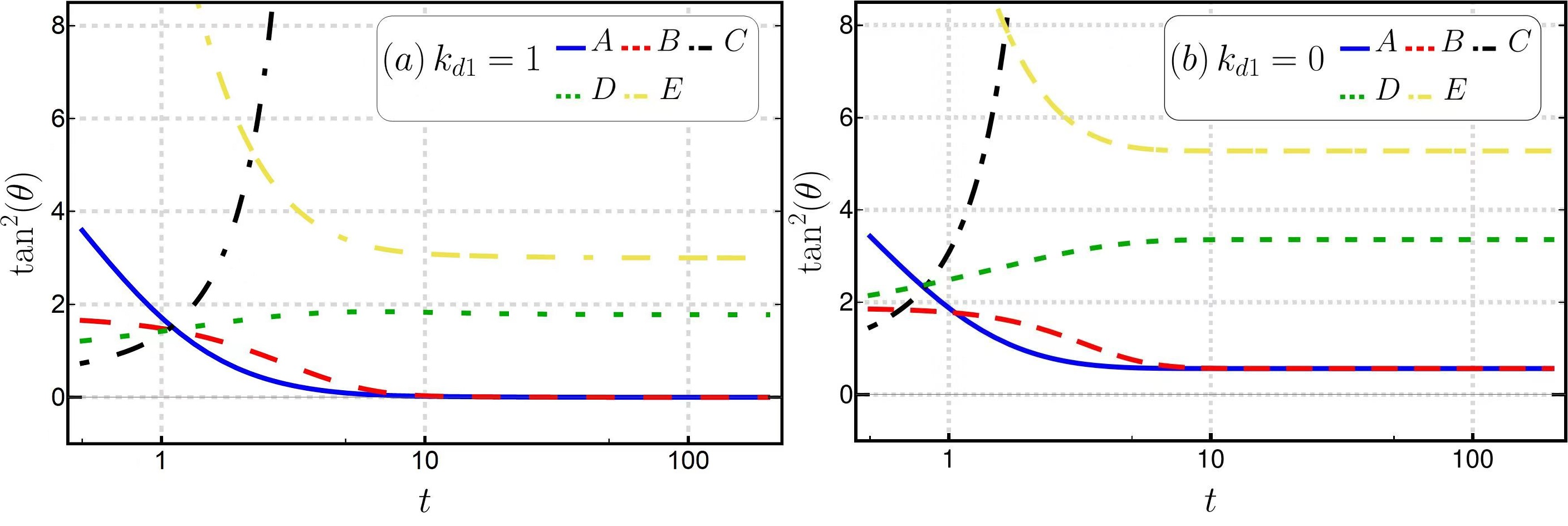
Because $d_{1}^{\pm}\geq 0$ and $d_{1}^{+}+d_{1}^{-}>0$ , $\Delta$ must not be less than 1 or $\Delta\geq 1$ , so $\Delta$ cannot be $2/\pi$ for the case $k_{d1}=0$ , which means that the CKWT state cannot be reached for $k_{d1}=0$ . For $k_{d1}>0$ , the CKWT state can be reached if and only if either of $d_{1}^{+}$ or $d_{1}^{-}$ is vanishing. This observation can be verified by the numerical results in Fig. 1 for different sets of values of $d_{1}^{\pm}$ and $d_{2}^{\pm}$ .

Refer to caption — Figure 1: Numerical results for $\tan^{2}(\theta)$ with two-band initial conditions for different set of amplitude values. The parameters are: $\eta=0.1$ , $k_{d1}=0\;\mathrm{or}\;1$ , $k_{d2}=2$ , $k_{d3}=4$ . A: $d_{1}^{+}=1$ , $d_{2}^{+}=1/4$ , $d_{1}^{-}=0$ , $d_{2}^{-}=1/4$ , B: $d_{1}^{+}=1/4$ , $d_{2}^{+}=1$ , $d_{1}^{-}=0$ , $d_{2}^{-}=1/4$ , C: $d_{1}^{+}=1/4$ , $d_{2}^{+}=1$ , $d_{1}^{-}=1/4$ , $d_{2}^{-}=0$ , D: $d_{1}^{+}=1$ , $d_{2}^{+}=1/4$ , $d_{1}^{-}=1/4$ , $d_{2}^{-}=0$ , E: $d_{1}^{+}=1$ , $d_{2}^{+}=1/4$ , $d_{1}^{-}=1/3$ , $d_{2}^{-}=1/3$ . (a) $k_{d1}=1$ . In case A and B, $\tan^{2}(\theta)$ tends to zero as $t\rightarrow\infty$ indicating that the CKWT state can be reached, while $\tan^{2}(\theta)$ tends to infinity, $16/9$ and $3$ as $t\rightarrow\infty$ in case C, D and E, respectively, which indicates that the CKWT state cannot be reached. (b) $k_{d1}=0$ . The CKWT state cannot be reached in all cases.

V.1.3 Multi-band functions

We now generalize two-steps functions to multi-steps functions,

\displaystyle g_{+}\left(0,k\right)

\displaystyle=\begin{cases}d_{1}^{+},&\mathrm{for}\;\;k_{d1}\leq k<k_{d2}\\ d_{2}^{+},&\mathrm{for}\;\;k_{d2}\leq k<k_{d3}\\ ...&...\\ d_{n}^{+},&\mathrm{for}\;\;k_{d(n)}\leq k<k_{d(n+1)}\end{cases},

(41)

g_{-}\left(0,k\right)=\begin{cases}d_{1}^{-},&\mathrm{for}\;\;k_{d1}\leq k<k_{d2}\\ d_{2}^{-},&\mathrm{for}\;\;k_{d2}\leq k<k_{d3}\\ ...&...\\ d_{n}^{-},&\mathrm{for}\;\;k_{d(n)}\leq k<k_{d(n+1)}\end{cases},

(42)

where $k\geq 0$ , $k_{d(n+1)}>k_{d(n)}>...>k_{d2}>k_{d1}\geq 0$ , $d_{1}^{+}+d_{1}^{-}>0$ and $d_{i}^{\pm}\geq 0$ for $i=1,2,...,n$ . The result is similar to the case of two-bands functions,

\lim_{t\rightarrow\infty}\frac{WQ}{H^{2}}-1\rightarrow\begin{cases}\frac{\left(d_{1}^{+}+d_{1}^{-}\right)^{2}}{\left(d_{1}^{+}-d_{1}^{-}\right)^{2}}-1,&\mathrm{for}\;\;k_{d1}>0\\ \frac{\pi}{2}\frac{\left(d_{1}^{+}+d_{1}^{-}\right)^{2}}{\left(d_{1}^{+}-d_{1}^{-}\right)^{2}}-1,&\mathrm{for}\;\;k_{d1}=0\end{cases}.

(43)

We see that the limit for $WQ/H^{2}$ is also determined by the amplitudes of the lowest bands. Similar to the analysis in the previous subsection that the CKWT state can only be reached for $k_{d1}>0$ under the condition that either of $d_{1}^{+}$ or $d_{1}^{-}$ is vanishing. This observation can be verified by the numerical results in Fig. 2 for different sets of values of $d_{i}^{\pm}$ for $i=1,\cdots,4$ .

V.2 Analytic functions as initial conditions

Based on the previous discussion about step functions as initial conditions, it is natural to generalize it to the limit of infinitely small intervals, i.e. analytic functions. As discussed in the previous subsection, the starting point of the integral can make a difference in the limit of $WQ/H^{2}$ . In this subsection, we will do the same thing by distinguishing two cases: $a>0$ and $a=0$ for the starting point of the integral range $[a,\infty)$ .

V.2.1 Integration range $[a,\infty)$ with $a>0$

The physical quantities in our consideration are all in the integrated form

X=\int_{a}^{\infty}dkk^{n}e^{-2\eta tk^{2}}f(k),

(44)

where the lower bound $a$ of the integration range is a positive number, and $f(k)$ is an analytic function, meaning that the Taylor expansion is valid at any value $k_{0}$ in the range $[a,\infty)$ ,

f(k)=\sum_{n=0}^{\infty}\frac{1}{n!}\left(k-k_{0}\right)^{n}f^{(n)}(k_{0}).

(45)

For $W$ , $Q$ and $H$ which we are considering in this paper, $f(k)$ can be either $\phi(k)$ or $\varphi(k)$ ,

	$\displaystyle\phi(k)$	$\displaystyle=$	$\displaystyle g_{+}(0,k)+g_{-}(0,k),$
	$\displaystyle\varphi(k)$	$\displaystyle=$	$\displaystyle g_{+}(0,k)-g_{-}(0,k).$		(46)

So $W$ , $Q$ and $H$ can be put into the forms,

$\displaystyle W$	$\displaystyle=$	$\displaystyle\int_{a}^{\infty}dkk^{2}e^{-2\eta tk^{2}}\left[\sum_{n=0}^{\infty}\frac{1}{n!}\phi^{(n)}(a)\left(k-a\right)^{n}\right],$
$\displaystyle Q$	$\displaystyle=$	$\displaystyle\int_{a}^{\infty}dke^{-2\eta tk^{2}}\left[\sum_{n=0}^{\infty}\frac{1}{n!}\phi^{(n)}(a)\left(k-a\right)^{n}\right],$
$\displaystyle H$	$\displaystyle=$	$\displaystyle\int_{a}^{\infty}dkke^{-2\eta tk^{2}}\left[\sum_{n=0}^{\infty}\frac{1}{n!}\varphi^{(n)}\left(a\right)\left(k-a\right)^{n}\right].$	(47)

Then we obtain the long time limit

\lim_{t\rightarrow\infty}\frac{WQ}{H^{2}}-1\rightarrow\left[\frac{g_{+}^{(i)}(0,a)+g_{-}^{(i)}(0,a)}{g_{+}^{(i)}(0,a)-g_{-}^{(i)}(0,a)}\right]^{2}-1,

(48)

where one can explicitly define the derivative index $i$ ( $i\geq 0$ ) with the following two cases: (a) $i=\min(i_{+},i_{-})$ if $g_{+}(0,k)$ and $g_{-}(0,k)$ are all non-vanishing, where $i_{s}$ is the index denote for a lowest order $i_{s}$ -th derivative that makes $g_{s}^{(i_{s})}(0,a)$ non-vanishing with $s=\pm$ , respectively; (b) If one of $g_{+}(0,k)$ and $g_{-}(0,k)$ is vanishing, for example, $g_{+}(0,k)=0$ , then for a lowest order $i$ -th derivative $g_{-}^{(i)}(0,a)\neq 0$ . So is the case $g_{-}(0,k)=0$ .

We see that the CKWT can be reached at $t\rightarrow\infty$ if and only if either $g_{+}^{(i)}(0,a)$ or $g_{-}^{(i)}(0,a)$ is vanishing. The proof of the result (48) is given in Appendix A.

V.2.2 Integration range $[0,\infty)$

In this section we consider the integration range $[0,\infty)$ , in which $g_{+}(0,k)$ and $g_{-}(0,k)$ are analytic functions and can be expanded in a Taylor expansion. In the following we use the shorthand notation $g_{\pm}(k)$ for $g_{\pm}(0,k)$ .

At $k=0$ , the Taylor expansion of $\phi(k)$ and $\varphi(k)$ in Eq. (46) reads

	$\displaystyle\phi(k)$	$\displaystyle=$	$\displaystyle\phi(0)+\phi^{\prime}(0)k+\frac{1}{2}\phi^{\prime\prime}(0)k^{2}+...,$
	$\displaystyle\varphi(k)$	$\displaystyle=$	$\displaystyle\varphi(0)+\varphi^{\prime}(0)k+\frac{1}{2}\varphi^{\prime\prime}(0)k^{2}+....$		(49)

By switching the order of the summation and the integration, one can calculate the integration of every term,

	$\displaystyle\frac{1}{n!}\int_{0}^{\infty}e^{-2\eta tk^{2}}\phi^{(n)}(0)k^{p+n}dk$	$\displaystyle\propto t^{-(1+p+n)/2},$
	$\displaystyle\frac{1}{n!}\int_{0}^{\infty}e^{-2\eta tk^{2}}\varphi^{(n)}(0)k^{1+n}dk$	$\displaystyle\propto t^{-(2+n)/2},$		(50)

where $p=0,2$ for $Q,W$ respectively. One can get rid of the term $t^{-(1+p+n)/2}$ for $n>i$ when $t$ goes to infinity, where $i$ is the the derivative index denote for a lowest order $i$ -th ( $i\geq 0$ ) derivative that makes $\phi^{(i)}(0)$ non-vanishing.

Similarly, we obtains the final result

\lim_{t\rightarrow\infty}\frac{WQ}{H^{2}}-1\rightarrow\left[\frac{g_{+}^{(i)}(0)+g_{-}^{(i)}(0)}{g_{+}^{(i)}(0)-g_{-}^{(i)}(0)}\right]^{2}\frac{\Gamma\left(\frac{3+i}{2}\right)\Gamma\left(\frac{1+i}{2}\right)}{\Gamma\left(\frac{2+i}{2}\right)\Gamma\left(\frac{2+i}{2}\right)}-1.

(51)

One can prove that the first factor in the right-hand-side of Eq. (51) is always larger than or equal to 1, and it is 1 if and only if either $g_{+}^{(i)}(0)=0$ or $g_{-}^{(i)}(0)=0$ . The second factor can be easily proved to be larger than 1. As a consequence, $WQ/H^{2}$ is always larger than 1 and will not reach $1$ as $t\rightarrow\infty$ , so the CKWT state cannot be reached in this case.

We see that the result for $a>0$ cannot be simply extended to that for $a=0$ by taking the limit $a\rightarrow 0$ . The analytical result can be verified numerically as presented in Fig. 3.

V.3 Special non-analytic function

For non-analytic functions as initial conditions, it is difficult to reach a similar conclusion as in previous sections. We can only take an example and carry out our numerical calculations. We consider the following function as the initial condition

g_{+}(0,k)=\begin{cases}e^{-1/k^{2}},&k>0\\ 0,&k=0\end{cases}.

(52)

What is special for this function is that it has infinite order of derivatives at $k=0$ which are vanishing. Thus $g_{+}(0,k)$ is non-analytic at $k=0$ and cannot be expanded into a Taylor series because zero is the essential singularity in the complex domain. For convenience, we assume $g_{-}(0,k)=0$ and the integration range is $[0,\infty)$ , then we can calculate $WQ/H^{2}$ directly and find the long time limit with the second kind modified Bessel function $K_{\nu}(z)$

\displaystyle\lim_{t\rightarrow\infty}\frac{WQ}{H^{2}}-1=\lim_{t\rightarrow\infty}\frac{e^{-4\sqrt{2\eta t}}\pi\left(1+2\sqrt{2\eta t}\right)}{16\eta t\left[K_{1}(2\sqrt{2\eta t})\right]^{2}}-1

\displaystyle\rightarrow

\displaystyle 0.

(53)

We see that under this condition the CKWT state can be reached.

VI Conclusion

We have studied how the Chandrasekhar-Kendall-Woltjer-Taylor (CKWT) state can be reached in the time evolution of a resistive plasma. We propose a criterion for the CKWT state as the destination of the time evolution, $\lim_{t\rightarrow\infty}\tan^{2}(\theta)\rightarrow 0$ , where $\theta$ is the average angle between the magnetic field and the vector potential. We find that the initial conditions for the helicity amplitudes of the magnetic field and the vector potential are essential to the CKWT state. Our analysis is based on an expansion in the vector spherical harmonics for magnetic fields and vector potentials.

The asymptotic form of $\tan^{2}(\theta)$ is dominated by the lowest momentum $k_{\mathrm{min}}$ of the initial helicity amplitudes $g_{\pm}(0,k)$ as functions of the scalar momentum $k$ . For those initial helicity amplitudes that can be expanded into a Taylor series, the CKWT state cannot be reached if $k_{\mathrm{min}}=0$ , while it can be reached for $k_{\mathrm{min}}>0$ if and only if either $g_{+}^{(i)}(0,k_{\mathrm{min}})=0$ or $g_{-}^{(i)}(0,k_{\mathrm{min}})=0$ with the lowest $i$ -th non-zero derivative ( $i\geq 0$ ) explained in Section V. In other words, the CKWT state can be reached if one helicity is favored over the other at the lowest momentum in the initial helicity amplitudes of the magnetic field. This indicates that the imbalance between two helicities at the lowest momentum (longest wavelength) in the initial helicity amplitudes is the key factor for the CKWT state.

Acknowledgments. Z.Y.Z., Y.G.Y. and Q.W. are supported in part by National Natural Science Foundation of China (NSFC) under Grant Nos. 12135011, 11890713 (a subgrant of 11890710) and 12047502, and by the Strategic Priority Research Program of Chinese Academy of Sciences under Grant No. XDB34030102.

References

Robinson (1969) D. C. Robinson, Plasma Physics 11, 893 (1969).
Bodin and Newton (1980) H. A. B. Bodin and A. A. Newton, Nuclear Fusion 20, 1255 (1980).
Ortolani and Schnack (1993) S. Ortolani and D. Schnack, Magnetohydrodynamics of Plasma Relaxation (World Scientific, 1993).
Sarff et al. (1997) J. S. Sarff, N. E. Lanier, S. C. Prager, and M. R. Stoneking, Phys. Rev. Lett. 78, 62 (1997).
Yagi et al. (1999) Y. Yagi, H. Sakakita, T. Shimada, K. Hayase, Y. Hirano, I. Hirota, S. Kiyama, H. Koguchi, Y. Maejima, T. Osakabe, Y. Sato, S. Sekine, and K. Sugisaki, Plasma Physics and Controlled Fusion 41, 255 (1999).
Sarff et al. (2003) J. Sarff, A. Almagri, J. Anderson, T. Biewer, A. Blair, M. Cengher, B. Chapman, P. Chattopadhyay, D. Craig, D. Den Hartog, et al., Nuclear Fusion 43, 1684 (2003).
Ding et al. (2004) W. X. Ding, D. L. Brower, D. Craig, B. H. Deng, G. Fiksel, V. Mirnov, S. C. Prager, J. S. Sarff, and V. Svidzinski, Phys. Rev. Lett. 93, 045002 (2004).
Prager et al. (2005) S. Prager, J. Adney, A. Almagri, J. Anderson, A. Blair, D. Brower, M. Cengher, B. Chapman, S. Choi, D. Craig, et al., Nuclear Fusion 45, S276 (2005).
Lorenzini et al. (2009) R. Lorenzini, E. Martines, P. Piovesan, D. Terranova, P. Zanca, M. Zuin, A. Alfier, D. Bonfiglio, F. Bonomo, A. Canton, et al., Nature Physics 5, 570 (2009).
Beltrami (1889) E. Beltrami, Il Nuovo Cimento 25, 212 (1889).
Lüst and Schlüter (1954) R. Lüst and A. Schlüter, Zeitschrift für Astrophysik 34, 263 (1954).
Chandrasekhar and Kendall (1957) S. Chandrasekhar and P. C. Kendall, Astrophys. J. 126, 457 (1957).
Chandrasekhar and Woltjer (1958) S. Chandrasekhar and L. Woltjer, Proceedings of the National Academy of Science 44, 285 (1958).
Woltjer (1958) L. Woltjer, Proceedings of the National Academy of Science 44, 489 (1958).
Wells and Norwood (1969) D. R. Wells and J. Norwood, Journal of Plasma Physics 3, 21–46 (1969).
Moffatt (1978) H. K. Moffatt, Magnetic Field Generation in Electrically Conducting Fluids, Cambridge Monographs on Mechanics (Cambridge University Press, 1978).
Berger and Field (1984) M. Berger and G. Field, Journal of Fluid Mechanics 147, 133–148 (1984).
Arnold and Khesin (1999) V. Arnold and B. Khesin, Topological Methods in Hydrodynamics, Applied Mathematical Sciences (Springer, New York, 1999).
Taylor (1974) J. B. Taylor, Phys. Rev. Lett. 33, 1139 (1974).
Taylor (1986) J. B. Taylor, Rev. Mod. Phys. 58, 741 (1986).
Schnack (2009) D. Schnack, Lectures in Magnetohydrodynamics: With an Appendix on Extended MHD, Lecture Notes in Physics (Springer, Berlin, Heidelberg, 2009).
Caramana et al. (1983) E. Caramana, R. Nebel, and D. Schnack, The Physics of Fluids 26, 1305 (1983).
Schnack et al. (1985) D. Schnack, E. Caramana, and R. Nebel, The Physics of Fluids 28, 321 (1985).
Strauss (1985) H. Strauss, The Physics of Fluids 28, 2786 (1985).
Kusano and Sato (1987) K. Kusano and T. Sato, Nuclear Fusion 27, 821 (1987).
Holmes et al. (1988) J. Holmes, B. Carreras, P. Diamond, and V. E. Lynch, The Physics of Fluids 31, 1166 (1988).
Ho and Craddock (1991) Y. Ho and G. Craddock, Physics of Fluids B: Plasma Physics 3, 721 (1991).
Diamond and Malkov (2003) P. Diamond and M. Malkov, Physics of Plasmas 10, 2322 (2003).
Marrelli et al. (2005) L. Marrelli, L. Frassinetti, P. Martin, D. Craig, and J. Sarff, Physics of Plasmas 12, 030701 (2005).
Bhattacharjee et al. (1980) A. Bhattacharjee, R. L. Dewar, and D. A. Monticello, Phys. Rev. Lett. 45, 347 (1980).
Bhattacharjee and Dewar (1982) A. Bhattacharjee and R. L. Dewar, The Physics of Fluids 25, 887 (1982).
Qin et al. (2012) H. Qin, W. Liu, H. Li, and J. Squire, Phys. Rev. Lett. 109, 235001 (2012).
Hirono et al. (2015) Y. Hirono, D. Kharzeev, and Y. Yin, Phys. Rev. D 92, 125031 (2015), arXiv:1509.07790 [hep-th] .
Vilenkin (1980) A. Vilenkin, Phys. Rev. D 22, 3080 (1980).
Kharzeev et al. (2008) D. E. Kharzeev, L. D. McLerran, and H. J. Warringa, Nucl. Phys. A 803, 227 (2008), arXiv:0711.0950 [hep-ph] .
Fukushima et al. (2008) K. Fukushima, D. E. Kharzeev, and H. J. Warringa, Phys. Rev. D 78, 074033 (2008), arXiv:0808.3382 [hep-ph] .
Kharzeev et al. (2013) D. E. Kharzeev, K. Landsteiner, A. Schmitt, and H.-U. Yee, Lect. Notes Phys. 871, 1 (2013), arXiv:1211.6245 [hep-ph] .
Kharzeev et al. (2016) D. E. Kharzeev, J. Liao, S. A. Voloshin, and G. Wang, Prog. Part. Nucl. Phys. 88, 1 (2016), arXiv:1511.04050 [hep-ph] .
Xia et al. (2016) X.-l. Xia, H. Qin, and Q. Wang, Phys. Rev. D 94, 054042 (2016), arXiv:1607.01126 [nucl-th] .
Chen and Fan (2013) J.-h. Chen and H.-y. Fan, Phys. Rev. Lett. 110, 269501 (2013).
Poincaré (1890) H. Poincaré, American Journal of Mathematics 12, 211 (1890).
Jackson (1999) J. D. Jackson, Classical electrodynamics, 3rd ed. (Wiley, New York, 1999).

Appendix A Proof of Eq. (48)

Using the asymptotic series of the incomplete gamma function $\Gamma(s,z)$ when $z\rightarrow\infty$ we obtain

	$\displaystyle\int_{a}^{\infty}k^{p}e^{-2k^{2}\eta t}dk$	$\displaystyle=$	$\displaystyle\frac{1}{2}(2\eta t)^{-(p+1)/2}\Gamma\left(\frac{1+p}{2},2a^{2}\eta t\right)$		(54)
		$\displaystyle\sim$	$\displaystyle e^{-2a^{2}\eta t}\sum_{j=1}^{\infty}\frac{a^{p-(2j-1)}}{(4\eta t)^{j}}\prod_{h=1}^{j-1}\left[p-\left(2h-1\right)\right],$		(54)

where the index $j$ is called the integral approximation order. The integration of the $i$ -th order term of Taylor expansion of $f(k)$ is evaluated as

	$\displaystyle X_{i}$	$\displaystyle=\int_{a}^{\infty}k^{n}\left[\frac{1}{i!}(k-a)^{i}f^{(i)}(a)\right]e^{-2k^{2}\eta t}dk$
		$\displaystyle=\frac{1}{i!}f^{(i)}(a)\sum_{m=0}^{i}C_{i}^{m}\left(\int_{a}^{\infty}k^{n+m}e^{-2k^{2}\eta t}dk\right)a^{i-m}(-1)^{i-m},$		(55)

where $n=0,1,2$ for $Q,H,W$ respectively.

Now we consider the $j$ -th order term in $X_{i}$ with the expansion of $\int_{a}^{\infty}k^{n+m}e^{-2k^{2}\eta t}dk$ following Eq. (54),

$\displaystyle X_{ij}$	$\displaystyle=$	$\displaystyle\frac{1}{i!}f^{(i)}(a)\sum_{m=0}^{i}C_{i}^{m}e^{-2a^{2}\eta t}\frac{a^{n+m-(2j-1)}}{(4\eta t)^{j}}$	(56)
		$\displaystyle\times\prod_{h=1}^{j-1}\left[n+m-(2h-1)\right]a^{i-m}(-1)^{i-m}$
	$\displaystyle=$	$\displaystyle\frac{1}{i!}f^{(i)}(a)e^{-2a^{2}\eta t}\frac{a^{n+i-(2j-1)}}{(4\eta t)^{j}}$
		$\displaystyle\times\sum_{m=0}^{i}C_{i}^{m}(-1)^{i-m}\left(\prod_{h=1}^{j-1}\left[n+m-(2h-1)\right]\right)$
	$\displaystyle=$	$\displaystyle\frac{1}{i!}f^{(i)}(a)e^{-2a^{2}\eta t}\frac{a^{n+i-(2j-1)}}{(4\eta t)^{j}}\sum_{m=0}^{j-1}i!S(m,i)q_{m}(j,n).$

Here we have used the second kind Stirling number $S(m,i)$ , with the function $q$ being defined as

\prod_{h=1}^{j-1}\left[n+m-(2h-1)\right]=\sum_{i^{\prime}=0}^{j-1}q_{i^{\prime}}(j,n)m^{i^{\prime}}.

(57)

Since $S(m,i)=0$ for $m<i$ , the lowest order term of $1/t$ among $X_{ij}$ must require $j=i+1$ with the lowest $i$ -th non-zero derivative ( $i\geq 0$ ), which is

f^{(i)}(a)e^{-2a^{2}\eta t}\frac{a^{n-i-1}}{(4\eta t)^{i+1}}.

(58)

And then as $t$ goes to infinity, the leading term of $WQ/H^{2}$ becomes

	$\displaystyle\frac{WQ}{H^{2}}$	$\displaystyle\sim\frac{\phi^{(i)}(a)e^{-2a^{2}\eta t}\frac{a^{1-i}}{(4\eta t)^{i+1}}\phi^{(i)}(a)e^{-2a^{2}\eta t}\frac{a^{-1-i}}{(4\eta t)^{i+1}}}{\varphi^{(i)}(a)e^{-2a^{2}\eta t}\frac{a^{-i}}{(4\eta t)^{i+1}}\varphi^{(i)}(a)e^{-2a^{2}\eta t}\frac{a^{-i}}{(4\eta t)^{i+1}}}$
		$\displaystyle=\left[\frac{\phi^{(i)}(a)}{\varphi^{(i)}(a)}\right]^{2},$		(59)

where $\phi^{(i)}(a)$ and $\varphi^{(i)}(a)$ are the same $i$ -th order derivatives of $\phi(k)$ and $\varphi(k)$ defined in Eq. (46) at $k=a$ .