Chandra observations of nova KT Eridani in outburst
Abstract
We analyse here four observations of nova KT Eri (Nova Eri 2009) done with the Chandra High Resolution Camera Spectrometer (HRC-S) and the Low Energy Transmission Grating (LETG) in 2010, from day 71 until day 159 after the optical maximum, in the luminous supersoft X-ray phase. The spectrum presents many absorption features with a large range of velocity, from a few hundred km s-1 to 3100 km s-1 in the same observation, and a few prominent emission features, generally redshifted by more than 2000 km s-1. Although the uncertainty on the distance and the WD luminosity from the approximate fit do not let us rule out a larger absolute luminosity than our best estimate of erg s-1, it is likely that we observed only up to 40% of the surface of the white dwarf, which may have been partially hidden by clumpy ejecta. Our fit with atmospheric models indicate a massive white dwarf in the 1.15-1.25 M⊙ range. A thermal spectrum originating in the ejecta appears to be superimposed on the white dwarf spectrum. It is complex, has more than one component and may be due to a mixture of photoionized and shock ionized outflowing material. We confirm that the 35 s oscillation that was reported earlier, was detected in the last observation, done on day 159 of the outburst.
keywords:
novae, cataclysmic variables, stars: individual (KT Eri), X-rays: stars1 Introduction
Novae in outburst are natural laboratories of extreme physical phenomena. They increase in optical luminosity from 8 to 17 magnitudes within hours, reach Eddington luminosity for a 1 M⊙ star (1038 erg s-1), and emit copious flux at all wavelengths, from radio to gamma rays. A recent observational review is the one by Poggiani (2018), while theoretical reviews can be found in Starrfield et al. (2012b); Starrfield et al. (2016) and Prialnik & Kovetz (2005). Nova eruptions are due to thermonuclear burning of hydrogen via the CNO cycle, at the bottom of a shell accreted by a white dwarf (WD) from a close binary companion. The outburst is repeated after periods ranging from a few years to hundreds of thousands years. Because the burning occurs in electron degenerate matter, it becomes explosive, inflating and possibly immediately ejecting part of the envelope. Since the initial suggestion of Bath & Shaviv (1976), it has been assumed that the bulk of the remaining envelope mass is then stripped by a radiation-pressure-driven wind, although a wind may also be triggered by Roche Lobe overflow (e.g., Wolf et al., 2013).
The evolutionary track of the post-nova is driven by a shift in the wavelength of the maximum energy toward shorter wavelengths, at a constant bolometric luminosity close to 1038 erg s-1 (e.g., Starrfield et al., 2012b; Wolf et al., 2013). Thus in X-rays, novae become some of the most luminous X-ray sources. The supersoft X-ray source (SSS) appears during post-maximum optical decline and lasts in different novae from one week to 10 years as the WD photosphere shrinks back to pre-outburst radius, while thermonuclear burning still occurs near the surface. The WD reaches effective temperature T250,000 K, so the energy peak is in the supersoft X-ray range. The SSS is indeed observed as predicted by the models (e.g., Orio, 2012). The SSS wavelength range is easily absorbed and if the column density exceeds 1022 cm-2, the WD may never be detected. In most cases, however, the filling factor of the ejecta is sufficiently low that the WD becomes a luminous X-ray source, observable with X-ray gratings as far as the Magellanic Clouds. By fitting atmospheric models abundances, effective temperature, white dwarf composition and mass can be derived. Novae in the SSS phase also exhibit time variability, both periodic and aperiodic (e.g., Ness et al. 2015 for the first, Orio et al. 2018 for the latter).
Nova outflows also emit X-rays, usually with a thermal spectrum, but they rarely are luminous enough to obtain a grating spectrum with good S/N ratio. However, the emission lines of the ejecta may be superimposed on the spectrum of the central source, complicating the spectral fitting. In the nova we examine in this article, KT Eri, the central source appeared to be dominant and have a relatively “clean” spectrum without a very large contribution of the ejecta.
Classical nova KT Eridani was discovered by Itagaki (2009) at V=8.1 on November 25.536 UT (MJD 55160.536), 2009. In a pre-discovery study Hounsell et al. (2010) found that the maximum was on 2009 November 14.67 at unfiltered Solar Mass Ejection Imager (SMEI) magnitude 5.420.02 and V=5.4 (Ootsuki et al., 2009), after a pre-maximum halt for a few hours at 6th SMEI magnitude, with a pre-outburst rise of by 3 magnitudes in 1.6 days. The outburst amplitude was 9 mag and the estimated time for a decay by 2 magnitudes was t2=6.6 days (Hounsell et al., 2010), indicating that KT Eri was a fast nova. KT Eri was spectroscopically classified as a “He/N nova”, implying characteristics that are not the most frequent in novae (Rudy et al., 2009), and are more often detected in recurrent novae. The ejecta velocity reached a maximum of 3400 km s-1 in H (Maehara & Fujii, 2009), and at later phases 2800200 km s-1 (Ribeiro et al., 2011). The distance is kpc, obtained thanks to the Gaia parallax111from the GAIA database using ARI’s Gaia Services at http://gaia.ari.uni-heidelberg.de/tap.html..
Ribeiro et al. (2013) modeled the evolution of the H profile, finding that the nova ejecta had the shape of a dumbbell structure with a ratio between the major to minor axis of 4:1, and an inclination angle of 58. From infrared observations, Raj et al. (2013) estimated an upper limit for the mass of the ejecta in the range 2.4–7.4 M, but this range should be decreased by a factor of 3 to account for the fact that the authors assumed a larger distance than the GAIA limits imply. Drake et al. (2009) detected a variable progenitor and Jurdana-Šepić et al. (2012) found that at quiescence the variability had a 1 mag amplitude, with two distinct periods of 376 and 737 days. These authors also noted the similarity of the KT Eri outburst with those of known recurrent novae, but could not find any previous outburst in the Harvard plates and suggested that the outbursts may recur on timescales of few centuries. They also found evidence that the progenitor is very likely to be an evolved star, ascending towards the red giant branch.
KT Eri was first detected as an X-ray source in outburst with the Swift XRT on day 39.8 after optical maximum, as a relatively hard source (Bode et al., 2010). It was still hard on day 47.5, but by day 55.4 a luminous SSS emerged. On day 65.6 the SSS was softened dramatically. Bode et al. (2010) noted that the time-scale for the SSS turn-on was very similar in the recurrent nova LMC 2009a. The timing analysis of the Swift XRT data from day 66.60 to 79.25 revealed a 35 s modulation (Beardmore et al., 2010), that was later confirmed by Ness et al. (2014, 2015) with Chandra. Ness et al. (2015) showed that this modulation was detected only during the early SSS phase, and then again much later, on day 159. With the Chandra LETG, the nova X-ray spectrum had several similarities with that of N SMC 2016 (Orio et al., 2018), with the luminous continuum and deep absorption lines of many novae X-ray spectra (Ness et al., 2010).
2 Observation and data reduction
KT Eri was observed by the HRC-S and the LETG of Chandra four times in 2010. The details of the observations are shown in Table 1. The principal investigator of the first observation was Jan-Uwe Ness (Ness et al., 2010), and Jeremy Drake was the principal investigator of the three following ones. The net exposure time for the first observation was about 15 ks, while the other three observations were shorter: the nominal exposures were to be of 5 ks, but some events could not be telemetered and the dead time corrected exposures were only of about 3 ks.
The Chandra X-ray data analysis software CIAO v4.11 and calibration package CALDB 4.8.5 were used for the data reduction. The background subtracted light curves measured with the Chandra HRC-S camera (0 order) were extracted from event files with “DMEXTRACT”. The script “chandra-repro” was used to extracted the Chandra HRC-S+LETG high resolution spectra, and the script “combine-grating-spectra” was used to combine the first order grating redistribution matrix files (rmf), ancillary response files (arf) and the grating spectra.
| Instrument | Datea | ObsID | Dayb | Exp. timec | C.R. (LETG) | C.R. (HRC-S) | Fx |
|---|---|---|---|---|---|---|---|
| (UTC) | (ks) | (counts s-1) | (counts s-1) | (erg s-1 cm-2) | |||
| Chandra HRC-S+LETG | 2010 Jan 23 | 12097 | 71.3 | 14.950 | 19.390.04 | 13.87 | 0.95 |
| Chandra HRC-S+LETG | 2010 Jan 31 | 12100 | 79.3 | 2.753 | 111.700.24 | 84.85 | 5.94 |
| Chandra HRC-S+LETG | 2010 Feb 06 | 12101 | 84.6 | 3.520 | 74.480.18 | 58.20 | 3.89 |
| Chandra HRC-S+LETG | 2010 Apr 21 | 12203 | 158.8 | 3.206 | 130.300.23 | 113.74 | 7.89 |
Notes: a: Start date of the observation. b: Time in days after the optical-maximum on 2009-11-13. c: Exposure time of the observation (dead time corrected).
3 Timing analysis
The background subtracted zero order light curves measured with the HRC-S camera, binned every 20 s for visual purposes, are shown in Fig. 1. The nova was also monitored with Swift and in Fig. 2 we show the Swift X-Ray Telescope (XRT) light curve and the AAVSO optical light curve in the visual and V band. The Swift XRT exposures were typically about 1000 s long.
The count rates vary significantly during all the four Chandra observations on relatively short time scales, and the average count rate also varied in the different exposures.
On day 71.3, the count rate varied by a factor of 7.8 during the exposure. On day 79.3 the variation was by a factor of 1.6, on day 84.6 by a factor of 3.9, on day 158.8 by a factor of 1.4.
3.1 Appearance and disappearance of a short periodic modulation
A period of 35 s was detected in the light curve of Swift XRT data by Beardmore et al. (2010). This period was only detected on the Chandra observation of day 158.8 by Ness et al. (2015). These authors calculated power spectra with the method of Horne & Baliunas (1986).
We confirm the detection, having found a period of s with 99.0% significance in the day 158.8 light curve. We used the Lomb–Scargle method (Scargle, 1982). We first detrended the light curves by subtracting the mean and dividing by the standard deviation. The Lomb-Scargle periodogram (LSP) was calculated by us with the Starlink PERIOD package. The PERIOD task SCARGLE was used to create a LSP of each light curve. The PERIOD task SCARGLE uses the Lomb–Scargle method by scanning in the frequency space. With SCARGLE we obtained the LSP frequency plot shown in the left panel of Fig. 3. With the PERIOD task PEAKS we found the highest peak in the periodogram between the frequencies we specified, and in order to determine the statistical significance of the period and obtain a statistical error, we performed a Fisher randomization test, as described by Linnell Nemec & Nemec (1985), over frequencies from 10 to 100 mHz, including also red noise in the significance analysis. The period was only detected in the light curve of the fourth observation. Considering that this period may have been missed if it was only present for a short time during an exposure, we divided the light curves of the other three observations into segments of 1000 s. A period of 35 s period was then detected in two segments of the first exposure, the eighth and the fourteenth in our subdivision in 1000 s intervals. However, the corresponding peaks in the periodogram are not very prominent. The results are shown in Table 2. No periodicity was retrieved in any of the intervals of the second and third exposure. Fig. 3 shows the LSP of the light curve on day 158.8 extracted with DMEXTRACT without any energy filtering and the same light curve folded on the corresponding detected period shown in Table 2.
| Observation | Period | Significance | Modulation |
|---|---|---|---|
| (or segment) | (s) | (%) | amplitudea (%) |
| day 71.3b (08)c | 67.5 | 4.52 | |
| day 71.3b (14)d | 85.5 | 9.68 | |
| day 158.8b | 99.0 | 2.18 |
Notes: a: We define the period modulation amplitude as . b: Time in days after the optical-maximum on 2009-11-13. c: Segment 8 in the exposure of day 71.3. d: Segment 14 in the exposure of day 71.3.
We did not detect any other periodicities in all four observations. The proposed periods of 0.09381 d (or 8105.18 s, Taichi Kato, vsnet-alert 11755222http://ooruri.kusastro.kyoto-u.ac.jp/mailarchive/vsnet-alert/11755.) and d ( s, Bruch 2018), detected in the optical light curves, are too long to be measured in the Chandra exposures.


4 The high resolution X-ray spectra
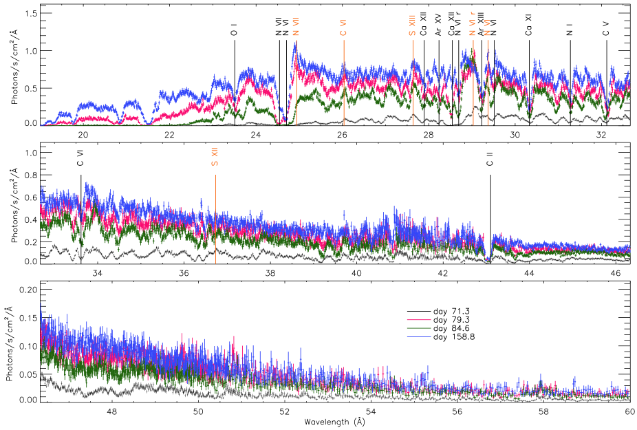
In Fig. 4 we show the summed +1 and -1 order LETG spectra of the four observations, and we indicate a number of clearly detected absorption and emission lines; these are the strongest ones.
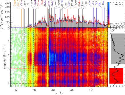
Fig. 5 illustrates the spectral evolution during the two exposures with large flux variations, which also presented spectral variations with the flux, namely day 71.3 (top row) and day 84.6 (bottom row). The respective plots on the left are the observed spectra, and on the right we show the time maps normalized to a blackbody curve that approximately fits the continuum. We first found the best fit blackbody curve for each observation, shown in the top left panel of the original time map with the dashed blue line, and following the blackbody we adjusted the normalization for the respective spectra. In the central panel for day 71.3 the N vi line at 28.79 Å grows after hours, while the zero-order light curve indicates this happened during an episode of still rather low count rate, before a rise. In the blackbody-normalized time map, this emission line appears more constant, indicating that it has grown together with the underlying continuum. However, hours after the beginning of the exposure, this line has shrunk considerably more than the continuum. We also note that at the same time, the continuum shortward of Å (possibly related to the C vi ionization edge at 25.3 Å) has decreased notably while some emission lines at long wavelengths (e.g., 31.8 Å, 32.8 Å, 41 Å, possibly S xiii and C v) have increased in strength. Thus, the emission lines above the continuum have thus not evolved in correlation or anti-correlation with the strength of the continuum.
Similarly, on day 84.6, the evolution of emission lines is not aligned with that of the continuum. During the brightest part of the light curve, hour after the beginning of the exposure (grey-shaded area in the bottom right panel), the N vi line at 28.78 Å has become slightly weaker relative to the continuum (thus has not increased in flux as much as the continuum) while shortward of 23 Å (possibly related to O i ionization edge in the cool gas), a few emission features have grown substantially. Possibly, the higher count rate was caused by a temporary reduction of the neutral oxygen column density. The surrounding cool material may be inhomogeneous, or it may have been temporarily ionized which would make it more transparent to high-energy radiation.


5 The individual lines: identification, fluxes, blue and red shift
We found absorption lines due to transitions of nitrogen, carbon, calcium and argon in all four spectra. The method described by Ness (2010); Ness et al. (2011) was used to determine the line shifts, widths, and optical depths at the line center of the absorption lines for the spectra for the four exposures. Following Ness et al. (2011), we did not include the absorption correction, because it is not important in determining velocity and optical depth. The narrow spectral region around each line is fitted with a function
| (1) |
.
Following Ness et al. (2011), the optical depth is defined as the Equation (2) in Ness (2010), and and in this equation are the central wavelength and the Gaussian line width which is always larger than the instrumental broadening, respectively. We assumed is a linear function for each line in modelling the continuum. We did compare the result with a continuum modelled with an absorbed black-body model and an absorbed TMAP model, and found that the model chosen for the continuum in the small wavelength range subtended by each line does not change the results. The Gaussian width of each line in velocity space was computed as , where c is the speed of light, is the central wavelength, and is the instrumental line broadening. This varies with the wavelength, as the LETG resolution is 0.05 Å. The resulting parameters for the blue shift velocity, broadening and optical depth at which each line is formed are shown in Table 3. If our line identification is right, there is a large spread of blue-shift velocities, from 370 to 3100 km s-1. While in some other novae, such as V2491 Cyg, RS Oph (Ness, 2010) and SMC 2016 (Orio et al., 2018), the blue-shift velocity of the absorption lines has a narrow variation range, there are at least three velocity systems in the spectra of V4743 Sgr (Ness et al., 2011).
The broadening of the lines also varies, and is larger than the instrumental width and broadening (expected to be less than 300 km s-1), so like in V2491 Cyg (Ness et al., 2011) the lines may have been produced in a region of plasma with a significant extension, allowing us to view a range of expansion velocities and thus a range of different plasma layers.
| Ion | |||||||||
| (Å) | (Å) | (km s-1) | (km s-1) | (Å) | (km s-1) | (km s-1) | |||
| Day 71.3 | Day 79.3 | ||||||||
| N VII | 24.779 | ||||||||
| N VI | 24.898 | ||||||||
| Ca XII | 27.973 | ||||||||
| Ar XV | 28.346 | ||||||||
| Ca XII | 28.681 | ||||||||
| N VI r | 28.787 | ||||||||
| Ar XIII | 29.497 | ||||||||
| N VI | 29.535 | ||||||||
| Ca XI | 30.448 | ||||||||
| C V | 32.400 | ||||||||
| C VI | 33.734 | ||||||||
| Day 84.6 | Day 158.8 | ||||||||
| N VII | 24.779 | ||||||||
| N VI | 24.898 | ||||||||
| Ca XII | 27.973 | ||||||||
| Ar XV | 28.346 | ||||||||
| Ca XII | 28.681 | ||||||||
| N VI r | 28.787 | ||||||||
| Ar XIII | 29.497 | ||||||||
| N VI | 29.535 | ||||||||
| Ca XI | 30.448 | ||||||||
| C V | 32.400 | ||||||||
| C VI | 33.734 | ||||||||


The absorption lines of N VII ( Å) and N VI ( Å) are blended, generating a flat bottom in the spectrum of day 84.6. Moreover, the N VI ( Å) has the largest optical depth it is saturated in all spectra. We derived wavelength, line shifts, widths, and optical depths by assuming an overlap of the lines, as shown in Fig. 6, and propose the possible fit for the spectra of days 79.3 and 158.8, but in the third observation the lines are detected, yet we were not able to obtain a fit. Even if the fit is acceptable, this blending introduces a large uncertainty.
We also identified emission lines of nitrogen, carbon and sulfur in all four spectra. As shown in Table 4, these emission lines are red-shifted with velocities in a large range, 1700-3200 km s-1. We used a Gaussian model (AGAUSS in XSPEC) to fit the profiles of the emission lines to determine the measured wavelength, line width and line shifts, modeling the underlying continuum with TMAP as shown in the next Section (even in this case, however, the choice of continuum is not critical). The AGAUSS model in XSPEC computes the line profile as follows:
| (2) |
where and are the line central wavelength in Angstrom and the instrumental broadening corrected line width in Angstrom, respectively. The resulting parameters are shown in Table 4. Table 5 also shows the difference in flux for the “high” and “low” periods defined for Fig. 9 for day 71.3. The emission lines that are strong enough to be identified are in the wavelength band 24 37 Å. The emission line N VII ( Å) merge in the continuum emission and is too weak to be identified in spectrum of day 71.3 which has the lowest count rate, but it can be identified in the spectra of the rest three observations. It is weak on day 84.6 when the count rate is low, and it is strong on days 79.3 and 158.8 when the count rates are high. The flux of emission line N VI r ( Å) on day 84.6 is higher than day 158.8 when the count rate is the highest. Therefore, the fluxes of the emission lines do not change monotonically with the count rate of the spectra.
Ness et al. (2013a) suggest that the emission lines in V2491 Cyg originated from the reprocessed emission far from the WD, in the clumpy ejecta of the nova wind. We also attribute them to the ejecta in KT Eri.
| Ion | Flux | Flux | |||||||
| (Å) | (Å) | (km s-1) | (km s-1) | (Å) | (km s-1) | (km s-1) | |||
| Day 71.3 | Day 79.3 | ||||||||
| N VII | 24.779 | … | … | … | … | 24.923 | 1747 | 1368 | 9.55 |
| C VI | 25.830 | 26.087 | 2987 | 640 | 0.80 | 26.079 | 2884 | 705 | 1.85 |
| S XIII | 27.392 | 27.653 | 2856 | 882 | 1.00 | 27.675 | 3016 | 433 | 2.65 |
| N VI r | 28.787 | 29.054 | 2780 | 1281 | 1.18 | 29.047 | 2783 | 839 | 8.93 |
| N VI | 29.084 | 29.348 | 2721 | 583 | 0.16 | 29.395 | 3205 | 364 | 2.92 |
| S XII | 36.398 | 36.767 | 3039 | 673 | 0.65 | 36.756 | 2948 | 509 | 0.62 |
| Day 84.6 | Day 158.8 | ||||||||
| N VII | 24.779 | 24.950 | 2069 | 328 | 0.89 | 24.947 | 2040 | 1914 | 16.40 |
| C VI | 25.830 | 26.056 | 2624 | 525 | 2.10 | 26.038 | 2416 | 574 | 1.57 |
| S XIII | 27.392 | 27.680 | 3147 | 1021 | 6.39 | 27.638 | 2696 | 1801 | 7.69 |
| N VI r | 28.787 | 29.031 | 2610 | 1075 | 9.42 | 29.030 | 2531 | 1016 | 3.99 |
| N VI | 29.084 | 29.346 | 2708 | 192 | 1.78 | 29.372 | 2969 | 244 | 2.78 |
| S XII | 36.398 | 36.786 | 3195 | 656 | 0.96 | 36.730 | 2734 | 467 | 0.20 |
| Ion | Flux (high) | Flux (low) | |
|---|---|---|---|
| (Å) | |||
| Day 71.3 | |||
| N VII | 24.779 | … | … |
| C VI | 25.830 | 0.86 | 0.39 |
| S XIII | 27.392 | 1.48 | 0.82 |
| N VI r | 28.787 | 1.56 | 0.85 |
| N VI | 29.084 | 0.28 | … |
| S XII | 36.398 | 0.91 | 0.49 |
6 Fits with comprehensive physical models
6.1 Fit with the TMAP library of atmospheric models
Fig. 8 shows the fit to the spectra of each exposure obtained with the fitting package XSPEC v 12.10.1 (Arnaud, 1996), with the TMAP model non-local thermodynamic equilibrium (NLTE) models (Rauch, 2003; Rauch et al., 2010) for an extremely hot WD atmosphere, as expected above a shell of ongoing thermonuclear burning. We used a public grid of calculated models with effective gravity indicated as log(g), varying between log(g)=5 and log(g)=9 (with a step increment of 1). These models were included as tables in XSPEC, using the tabular additive model ATABLE. Because the absorption features are blue-shifted, we assumed a constant blue shift for each absorption features except those originating in the cool gas of the intervening ISM. We found that the nova is so hot that only models with log(g)=9 are relevant, or else the luminosity would be largely above Eddington value. The Tuebingen-Boulder ISM absorption model TBABS (Wilms et al., 2000) in XSPEC was used to take the hydrogen column into account. Fig. 9 shows the fit to the “higher than average” and “lower than average” spectra of the first observation.
We first note that, on the blue or “hard” side, the flux in the spectrum of the first exposure appears to be cut by a K absorption edge of N VI (22.46 Å) while for the other 3 observations, the absorption edge that cuts the flux appears to be due to N VII at 18.59 Å, and this indicates lower temperature in the first observations. It also constrains the temperature in the last three exposures to be higher, and within a close range. The fits with TBABS+TMAP that minimize the parameters for all the observations are shown in Fig. 8 and Fig. 9, and the parameters are given in the Table 6. The minimum parameter divided by degrees of freedom was much larger than 1 (around 3 for the last three observations), so we could not conclude that these “best fits” are statistically good. In fact, many spectral features, especially those that we tentatively classify in emission could not be fitted. Moreover, as we discuss in detail in Section 5, the absorption features do not have all the same blueshift velocity and appear to have been produced at different optical depth, making a rigorous fit with the model infeasible. However, because the level and shape of the continuum are well reproduced, and so are the strongest absorption features, as shown in Fig. 8, the fit allows deriving important physical parameters. Although we used three different models of the TMAP grid, varying in nitrogen and carbon abundance, we caution that this does not necessarily indicate variation of these elements’ abundances mixed in the outer atmospheric layer. TMAP models only include the chemical composition of elements of H, He, C, N, O, Ne, Mg, Si, S, Ca and Ni, they lack the Ar element, while Ar L-shell ions are rather important between the energy range 20 - 40 Å and two absorption lines (Ar XV, Å; Ar XIII, Å) are identified in the spectra. Only an ad-hoc TMAP model for this nova, with abundances as free parameters and including different blueshift velocity for the lines, would allow fitting a larger number of lines and obtaining a statistically rigorous fit, but it requires extensive modeling that is beyond the scope of this observational paper.
For the average spectrum of day 71.3, by leaving all parameters free we obtained a N(H) value of 4.3 1020 cm-2, but because we could not reproduce the K-edge absorption edge of N VI at 22.46 Å that “cuts” the spectrum, we decided to constrain the N(H) value at 6 1020 cm-2, close to that obtained for the remaining epochs and to the column density in the direction of the nova indicated by HI4PI Collaboration et al. (2016), without even assuming any intrinsic absorption of the ejecta. Fig. 8 and Table 6 also show the spectral fit for the first exposure. The fit improved when we split the first observation into periods of "high" and "low" count rates, but we still had to constrain N(H) to reproduce the absorption edge. Most notably, for the first spectrum we could not explain excessive emission at 23-24 Å.
The best fit value of Teff of day 158.8, 805,000 K implies a WD mass in the range 1.15-1.25 M⊙ according to Yaron et al. (2005), about 1.25 M⊙ (following Starrfield et al., 2012a), or a little less than 1.2 M⊙ (according to Wolf et al., 2013). This is consistent also with the range estimated by Jurdana-Šepić et al. (2012) considering the lower limit on the recurrence time and on estimate of mass accretion rate .
The strongest absorption features are as deep as predicted by the TMAP model, and they are almost all blue-shifted (except the ISM features: O I, N I and C II), however, we show in the next Section that the blue shift velocity varies, but we only had uniform blue-shift velocity in the TMAP model fit. Moreover, some adjacent absorption lines are blended, complicating the fitting procedure. We considered the possibility that two models at different temperature and blue-shift velocity are needed for the fit, implying a non-uniform WD atmosphere with two different zones, but this attempt did not improve the fit.
These fits predict less flux (25% for the first observation, 5% for the others) than measured, indicating that one additional component is contributing to the flux. In other novae, this has been attributed to the shocked optically thin plasma of the ejecta (.e.g. N LMC 2009, Bode et al., 2016). In the first observation, clearly the optically thin plasma must be contributing more to the total flux budget. Values of X-ray luminosity of the ejecta of the order of 1034 erg s-1 are rather typical for non-symbiotic novae (Orio, 2012).
In order to fit the additional component, and especially the emission lines in the range 2030 Å with a wide range red-shifted velocity, we added a model of shocked plasma in collisional ionization equilibrium, that takes line shifts and line broadening into account, namely BVAPEC in XSPEC (Smith et al., 2001). Such a composite model had been found could fit the spectra of novae U Scorpii (Orio et al., 2013), T Pyxidis (Tofflemire et al., 2013), and V959 Mon (Peretz et al., 2016). In Fig. 10 we show the composite model fit for the first two observations, and the parameters are reported in Table 7. The fit is improved with the introduction a few strong emission features, but several other features are still unaccounted for. For the first observation the excess flux at the short wavelengths is better modeled by a complex of N VI and N VII lines, but the continuum level is not sufficiently high yet at these wavelengths.
The static model indicates that the peak luminosity (4.90 erg s-1. Assuming the unabsorbed flux of the last exposure’s spectral fit and the distance of kpc), the derived absolute luminosity is only a fraction of (less than 40%) the total X-ray luminosity of the WD. In fact, detailed calculations by Yaron et al. (2005) show that the bolometric luminosity (of which the X-ray luminosity at T K constitutes more than 95%), for a WD mass of at least 1 M⊙ it would always exceed 1.3 erg s-1.


| Day | Teff (K) | N(H) (1020 cm-2) | Velocity (km s-1)a | F(abs) | F(unabs) | [N/N⊙]b | [C/C⊙]b |
|---|---|---|---|---|---|---|---|
| (erg cm-2 s-1) | (erg cm-2 s-1) | ||||||
| 71.3 | 566,430 | 6.00 | 3029 | 0.71 | 6.01 | 1.668 | -0.057 |
| 71.3 (High)c | 571,493 | 6.00 | 3029 | 0.97 | 8.38 | 1.668 | -0.057 |
| 71.3 (Low)d | 559,860 | 6.00 | 3029 | 0.44 | 4.33 | 1.668 | -0.057 |
| 79.3 | 760,344 | 5.73 | 2771 | 5.48 | 23.95 | 1.803 | -1.513 |
| 84.6 | 721,063 | 5.61 | 1213 | 3.44 | 16.48 | 1.803 | -1.513 |
| 158.8 | 805,023 | 5.74 | 1126 | 7.55 | 30.12 | 1.678 | -1.073 |
Notes: a: The velocity of TMAP. b: Logarithm of abundance ratio.
c: Spectrum extracted for the
period during which the zero order light curve count rate was larger than the average 13.87 counts s-1. d: Spectrum extracted for the period
during which the zero order light curve count rate was lower than the average 13.87 counts s-1.
| Day | Teff (K) | N(H) (1020 cm-2) | Vbsa (km s-1) | Tbv (eV)b | Vrs (km s-1)c | vb (km s-1)d | [N/N⊙] | [C/C⊙] | [S/S⊙] |
|---|---|---|---|---|---|---|---|---|---|
| 71.3 | 560,517 | 6 (fixed) | 2999 | 81 | 2794 | 1500 | 1000 | 73 | 143 |
| 79.3 | 758,894 | 5.61 | 2737 | 150 | 2025 | 1074 | 1000 | 152 | 0.003 |
Notes: a: The velocity of TMAP. b: The temperature of BVAPEC. c: The centroid shift of BVAPEC. d: The broadening velocity of BVAPEC.
6.2 Fitting the spectrum with the “wind atmosphere” model
The other grid of models we used was obtained with the “wind-type” (WT) PHOENIX expanding atmosphere code, which includes a larger number of atomic species, but was developed only with solar abundances (van Rossum, 2012). Since abundances are very different from solar in the burning layer and burning ashes, and convection mixes this material abundantly in the WD atmosphere, this is of course a drawback in using the public model grid. The model assumes a hydrostatic base, parameterized with effective temperature Teff, radius R and gravitational acceleration log(g), and an envelope with a constant mass loss rate and a velocity v, with law similar to that of the winds of massive stars, namely
| (3) |
where =1.2 in order to have a smooth transition between the static core and the expanding envelope, and the asymptotic velocity v∞ is the fifth parameter of the public calculated grid. The values of are between 10-7 and 10-9 M⊙ yr-1, thus the mass loss is assumed to be quite small compared to the values during the nova outflows before the supersoft X-ray phase. At higher the lines are not just in absorption, but they have emission wings and a P-Cyg profile forms. On the other hand, the higher the temperature, the less prominent are these emission wings, and at the temperature of the novae observed so far, not many and not very strong emission wings are not produced in the atmosphere (see Orio et al., 2018). In addition, the large blue-shift velocities observed so far, exceeding 1000 km s-1, tend to smooth these P-Cyg profiles and make them difficult to detect and measure. In other words, we do not expect the WT model to explain the emission lines of the X-ray spectra of novae as formed in the atmosphere or in the wind close to the WD. They are more likely to be due to shocks and to form far from the WD surface (see also Ness et al., 2013a).
Other characteristics of the model are the much less prominent and smoother absorption edges, and because the configuration is not static, the effective gravity can be lower (due to a larger radius), since the outflow implies that balancing the radiation pressure is not required. Thus, g is smaller than in the static models with the same Teff. There is also very little dependence of the spectrum on the WD mass, because Teff is not a function of the mass as in the static models: the WD radius varies and is much larger than in the static configuration. Thus, it is interesting to experiment and try and fit the spectra also with this model, to see whether it better fits the continuum and the absorption features, accounting for their blue-shift.
We fitted the fluxed spectra (corrected for effective area) with the models of the WT grid in IDL. We did not attempt to choose a best fitting model by minimizing statistical parameter. Most models in the grid are inadequate and were ruled out immediately, since they predict high flux in a much broader wavelength range. In order to take the intervening column density into account, we used again the Tübingen-Boulder absorption model and performed the calculation with the related routine TBNEW in IDL.
Table 8 reports the parameters of the grid we chose because they fit better than others the continuum shape and the absorption edge causing abrupt flux decrease at the higher energy. The results are shown in Fig. 11. Because the high blue shift velocity smooths the absorption edges and lines excessively for this spectrum, we compensated by assuming a higher value of the absorbing column density, which would indicate some amount of intrinsic absorption in the ejecta. However, the N(H) value causes too little flux below 50-55 Å. We could not solve this problem and fit the hard and soft portion of the spectrum simultaneously. As expected, Teff is lower than that resulting from the TMAP best fit, and is of the order of 10-8 M⊙ yr-1. Altogether, TMAP fits the continuum and the strongest absorption lines much better than this model. We have interpolated between the tabulated models from van Rossum’s archive333http://flash.uchicago.edu/~daan/WT_SSS/, which were developed specifically for another nova (V4743 Sgr), so we were not expecting a perfect fit, but the large discrepancy between this model and observed spectra is disappointing. We note that, with larger absorbing column density N(H), in this model the unabsorbed flux in the last exposure reaches 7 erg cm-2 s-1, implying that a larger portion (less than 85%) of the WD was visible to us. However, the model shown in the figure overestimates the absorbed flux in the X-ray band (see comparison with Table 1).
| Day | Teff (K) | N(H) (1020 cm-2) | Velocity (km s-1) | log(g) (cm s-2) | (M⊙ year-1) | F(abs) (erg cm-2 s-1) |
|---|---|---|---|---|---|---|
| 71.3 | 475,000 | 9.70 | 2400 | 8.49 | 1.0 | 1.19 |
| 79.3 | 500,000 | 9.50 | 1800 | 7.77 | 7.6 | 6.21 |
| 84.6 | 475,000 | 8.50 | 2400 | 8.32 | 3.1 | 2.53 |
| 158.8 | 500,000 | 8.50 | 2400 | 7.73 | 1.0 | 8.81 |
7 Discussion
The X-ray luminosity of KT Eri and its variation is consistent with the possibility that we observed only a fraction of the WD surface, with visibility varying within hours. This seems to be a common phenomenon in many novae, and was observed, for instance, also in N LMC 2009 (Orio et al., 2021) and N SMC 2016 (Orio et al., 2018). Detailed calculations show that the thermonuclear runaway always expands all over the surface and is nearly spherically symmetric (Glasner et al., 1997), so the supersoft flux is also expected to be homogeneous in the WD surface, at least until the time magnetically driven accretion onto the WD is resumed on strongly magnetized WDs (see Aydi et al., 2018; Zemko et al., 2018). The likely explanation we propose for KT Eri is that there were dense clumps in the ejecta, which were optically thick to the X-rays. Although it may seem more likely to produce a clumpy outflow in the initial explosive emission, the SSS variation in KT Eri was observed so long after the outburst maximum that initial clumps must have been ejected far away from the WD, and be located where the WD would appear as a point source, so partial obscuration by these initial ejecta would be unlikely. We suggest that the optically thick radiation driven wind that is supposed to last for months (initially suggested by Bath & Shaviv, 1976, and always included in the nova models) is not a continuous and smooth phenomenon. Even if this variable wind has never been modeled, many data can be explained with distinct ejection episodes at different wind velocity, including observations of novae T Pyx (Chomiuk et al., 2014) and V906 Car (Sokolovsky et al., 2020). Distinct outflows may be a common occurrence also according to Aydi et al. (2020). Instabilities are likely to occur in such a “stunted” outflow, and may cause sufficiently small scale clumpiness to obscure only a portion of the WD, so that the filling factor of the ejecta along the line of sight varied within hours.
The X-ray grating spectra allow to draw some conclusions regarding the WD mass. van Rossum (2012) shows that the effect of an ongoing outflow is to lower the atmospheric temperature, and somewhat bloat the radius, reaching the same luminosity of a static configuration at lower Teff. However, because the full fledged evolutionary models of the outburst (e.g., MESA used by Wolf et al. (2013), or the model calculated by Yaron et al. (2005) and references therein) also assume a static atmosphere, from which mass loss has ceased at the peak of the supersoft X-ray phase, the results of the outburst models can be compared with the parameters derived with TMAP, which is also static. For KT Eri, from the TMAP fit we obtain a peak Teff of about 800,000 K, corresponding to a WD mass in the range 1.15 1.25 M⊙ according to all nova outburst models quoted above. It is interesting to notice that Jurdana-Šepić et al. (2012) estimated an approximate pre-outburst accretion rate from the optical B luminosity at quiescence, and by assuming a recurrence time of more than 100 years (because no previous outburst was found in the Harvard plates), these authors reached the same conclusion concerning the WD mass of KT Eri.
The above result is in agreement with the parameters derived correlating also additional observational evidence with the models. The Swift XRT light curve shows that the SSS flux decreased by a factor close to 16 in exactly 7 months after optical maximum. 210 days is thus the duration of the “bolometric t3” (time for a decrease by the equivalent of 3 mag in optical), which is the parameter adopted by Yaron et al. (2005) to evaluate the duration of the constant bolometric luminosity phase of a nova. This parameter turns out to be of the order of 200 days for a 1.25 M⊙ WD for a large range of initial WD surface temperature and for a pre-outburst mass accretion rate M⊙ yr-1, while a 1 M⊙ WD nova with the same “bolometric t3” would have been initially cool, and would have undergone mass transfer in a narrow range M⊙ yr M⊙ yr-1. We now know also the X-ray luminosity of KT Eri at quiescence: assuming that the X-rays originate in the boundary layer of a geometrically thin accretion disk, Sun et al. (2020) indeed derived a consistent value, M⊙ yr-1 9 years after the outburst, which can be regarded as a lower limit, because it may be higher if there is an accretion disk corona emitting only in the UV.
8 Conclusions
The spectra of novae in the X-ray supersoft phase are complex, but they contain a wealth of physical information. We found that the KT Eri spectrum has a range of blue shift velocity of the absorption lines and red shift velocity of the emission lines. By fitting models with a single velocity, the fit is driven by the strongest features. A future, comprehensive model should account also for absorption features produced in layers of different optical depth and velocity. We calculated the velocity of the strongest absorption features and optical depth at which they are produced, as useful data to study more complex physical models in the near future.
The analysis of the X-ray spectra of KT Eri is complicated by the large irregular variability in two of the exposures, and by the overlapping emission lines, which we attributed to the ejecta as suggested for most novae and SSS by Ness et al. (2013b). These emission lines are not predicted to originate from, or near, the WD by the static atmospheric models, neither by the wind-atmosphere models. In the static atmosphere, conspicuous emission lines are formed only for the lowest WD masses (Rauch et al., 2010), at much lower Teff than that resulting from the KT Eri spectra. The wind-atmosphere model of van Rossum (2012) instead predicts more emission lines and actual P-Cyg profiles, but they are smoothed and even “washed out” by the wind velocity. We could not model the emission line spectrum by adding one or two CIE components, and concluded that it is produced in a complex emission region, and perhaps it is not only due to shock ionization. In at least two exposures, the variation of the flux in some emission lines is independent of the variations of the continuum SSS flux and may be related by variations in the neutral oxygen column density. We suggested that either the surrounding cool material is not homogeneous, or that it was temporarily ionized.
Our analysis of these spectra was phenomenological and included the comparison with atmospheric, wind and outburst models. We were able to conclude that the nova WD has mass in the 1.15-1.25 M⊙ range and that the mass accretion rate before the outburst was most likely close to a value of 10-10 M⊙ yr-1.
Finally, we also confirmed that pulsations of the SSS with a 35 s timescale appeared only late in the post-outburst X-ray light curve, more than 100 days after optical maximum. We note that this was quite different from the case of RS Oph, in which a 35 s periodicity appeared only in the first 55 days after optical maximum (see Nelson et al., 2008; Osborne et al., 2011; Ness et al., 2013b), We suggest that the search for the root cause of this phenomenon will have to make use of this fact and correlate it with other differences in the physical parameters of the two novae.
Data Availability
The data analyzed in this article are all available in the HEASARC archive of NASA at the following URL: https://heasarc.gsfc.nasa.gov/db-perl/W3Browse/w3browse.pl
Acknowledgements
We thank the anonymous referee for her or his constructive comments and suggestions, which helped us to improve the scientific content of this paper. S. Pei has been supported by the China Scholarship Council (No. 201704910918) and M. Orio by a Chandra-Smithsonian grant for archival research at the University of Wisconsin.
References
- Arnaud (1996) Arnaud K. A., 1996, in Jacoby G. H., Barnes J., eds, Astronomical Society of the Pacific Conference Series Vol. 101, Astronomical Data Analysis Software and Systems V. p. 17
- Aydi et al. (2018) Aydi E., et al., 2018, MNRAS, 480, 572
- Aydi et al. (2020) Aydi E., et al., 2020, ApJ, 905, 62
- Bath & Shaviv (1976) Bath G. T., Shaviv G., 1976, MNRAS, 175, 305
- Beardmore et al. (2010) Beardmore A. P., et al., 2010, The Astronomer’s Telegram, 2423, 1
- Bode et al. (2010) Bode M. F., et al., 2010, The Astronomer’s Telegram, 2392, 1
- Bode et al. (2016) Bode M. F., et al., 2016, ApJ, 818, 145
- Bruch (2018) Bruch A., 2018, New Astron., 58, 53
- Chomiuk et al. (2014) Chomiuk L., et al., 2014, ApJ, 788, 130
- Drake et al. (2009) Drake A. J., et al., 2009, The Astronomer’s Telegram, 2331, 1
- Glasner et al. (1997) Glasner S. A., Livne E., Truran J. W., 1997, ApJ, 475, 754
- HI4PI Collaboration et al. (2016) HI4PI Collaboration et al., 2016, A&A, 594, A116
- Horne & Baliunas (1986) Horne J. H., Baliunas S. L., 1986, ApJ, 302, 757
- Hounsell et al. (2010) Hounsell R., et al., 2010, The Astronomer’s Telegram, 2558, 1
- Itagaki (2009) Itagaki K., 2009, Central Bureau Electronic Telegrams, 2050, 1
- Jurdana-Šepić et al. (2012) Jurdana-Šepić R., Ribeiro V. A. R. M., Darnley M. J., Munari U., Bode M. F., 2012, A&A, 537, A34
- Linnell Nemec & Nemec (1985) Linnell Nemec A. F., Nemec J. M., 1985, AJ, 90, 2317
- Maehara & Fujii (2009) Maehara H., Fujii M., 2009, Central Bureau Electronic Telegrams, 2053, 3
- Nelson et al. (2008) Nelson T., Orio M., Cassinelli J. P., Still M., Leibowitz E., Mucciarelli P., 2008, ApJ, 673, 1067
- Ness (2010) Ness J. U., 2010, Astronomische Nachrichten, 331, 179
- Ness et al. (2010) Ness J. U., Drake J. J., Starrfield S., Bode M., Page K., Beardmore A., Osborne J. P., Schwarz G., 2010, The Astronomer’s Telegram, 2418, 1
- Ness et al. (2011) Ness J. U., et al., 2011, ApJ, 733, 70
- Ness et al. (2013a) Ness J. U., et al., 2013a, A&A, 559, A50
- Ness et al. (2013b) Ness J. U., et al., 2013b, A&A, 559, A50
- Ness et al. (2014) Ness J. U., et al., 2014, The Astronomer’s Telegram, 6147, 1
- Ness et al. (2015) Ness J. U., et al., 2015, A&A, 578, A39
- Ootsuki et al. (2009) Ootsuki I., et al., 2009, IAU Circ., 9098, 2
- Orio (2012) Orio M., 2012, Bulletin of the Astronomical Society of India, 40, 333
- Orio et al. (2013) Orio M., et al., 2013, MNRAS, 429, 1342
- Orio et al. (2018) Orio M., et al., 2018, ApJ, 862, 164
- Orio et al. (2021) Orio M., et al., 2021, MNRAS, 505, 3113
- Osborne et al. (2011) Osborne J. P., et al., 2011, ApJ, 727, 124
- Peretz et al. (2016) Peretz U., Orio M., Behar E., Bianchini A., Gallagher J., Rauch T., Tofflemire B., Zemko P., 2016, ApJ, 829, 2
- Poggiani (2018) Poggiani R., 2018, in Accretion Processes in Cosmic Sources - II. p. 57
- Prialnik & Kovetz (2005) Prialnik D., Kovetz A., 2005, in Burderi L., Antonelli L. A., D’Antona F., di Salvo T., Israel G. L., Piersanti L., Tornambè A., Straniero O., eds, American Institute of Physics Conference Series Vol. 797, Interacting Binaries: Accretion, Evolution, and Outcomes. pp 319–330, doi:10.1063/1.2130250
- Raj et al. (2013) Raj A., Banerjee D. P. K., Ashok N. M., 2013, MNRAS, 433, 2657
- Rauch (2003) Rauch T., 2003, A&A, 403, 709
- Rauch et al. (2010) Rauch T., Orio M., Gonzales-Riestra R., Nelson T., Still M., Werner K., Wilms J., 2010, ApJ, 717, 363
- Ribeiro et al. (2011) Ribeiro V. A. R. M., Darnley M. J., Bode M. F., Munari U., Harman D. J., Steele I. A., Meaburn J., 2011, MNRAS, 412, 1701
- Ribeiro et al. (2013) Ribeiro V. A. R. M., Bode M. F., Darnley M. J., Barnsley R. M., Munari U., Harman D. J., 2013, MNRAS, 433, 1991
- Rudy et al. (2009) Rudy R. J., Prater T. R., Russell R. W., Puetter R. C., Perry R. B., 2009, Central Bureau Electronic Telegrams, 2055, 1
- Scargle (1982) Scargle J. D., 1982, ApJ, 263, 835
- Smith et al. (2001) Smith R. K., Brickhouse N. S., Liedahl D. A., Raymond J. C., 2001, ApJ, 556, L91
- Sokolovsky et al. (2020) Sokolovsky K. V., et al., 2020, MNRAS, 497, 2569
- Starrfield et al. (2012a) Starrfield S., Timmes F. X., Iliadis C., Hix W. R., Arnett W. D., Meakin C., Sparks W. M., 2012a, Baltic Astronomy, 21, 76
- Starrfield et al. (2012b) Starrfield S., Iliadis C., Timmes F. X., Hix W. R., Arnett W. D., Meakin C., Sparks W. M., 2012b, Bulletin of the Astronomical Society of India, 40, 419
- Starrfield et al. (2016) Starrfield S., Iliadis C., Hix W. R., 2016, PASP, 128, 051001
- Sun et al. (2020) Sun B., Orio M., Dobrotka A., Luna G. J. M., Shugarov S., Zemko P., 2020, MNRAS, 499, 3006
- Tofflemire et al. (2013) Tofflemire B. M., Orio M., Page K. L., Osborne J. P., Ciroi S., Cracco V., Di Mille F., Maxwell M., 2013, ApJ, 779, 22
- Wilms et al. (2000) Wilms J., Allen A., McCray R., 2000, ApJ, 542, 914
- Wolf et al. (2013) Wolf W. M., Bildsten L., Brooks J., Paxton B., 2013, ApJ, 777, 136
- Yaron et al. (2005) Yaron O., Prialnik D., Shara M. M., Kovetz A., 2005, ApJ, 623, 398
- Zemko et al. (2018) Zemko P., et al., 2018, MNRAS, 480, 4489
- van Rossum (2012) van Rossum D. R., 2012, ApJ, 756, 43