Certifying Some Distributional Fairness
with Subpopulation Decomposition
Abstract
Extensive efforts have been made to understand and improve the fairness of machine learning models based on different fairness measurement metrics, especially in high-stakes domains such as medical insurance, education, and hiring decisions. However, there is a lack of certified fairness on the end-to-end performance of an ML model. In this paper, we first formulate the certified fairness of an ML model trained on a given data distribution as an optimization problem based on the model performance loss bound on a fairness constrained distribution, which is within bounded distributional distance with the training distribution. We then propose a general fairness certification framework and instantiate it for both sensitive shifting and general shifting scenarios. In particular, we propose to solve the optimization problem by decomposing the original data distribution into analytical subpopulations and proving the convexity of the sub-problems to solve them. We evaluate our certified fairness on six real-world datasets and show that our certification is tight in the sensitive shifting scenario and provides non-trivial certification under general shifting. Our framework is flexible to integrate additional non-skewness constraints and we show that it provides even tighter certification under different real-world scenarios. We also compare our certified fairness bound with adapted existing distributional robustness bounds on Gaussian data and demonstrate that our method is significantly tighter.
1 Introduction
As machine learning (ML) has become ubiquitous [24, 18, 5, 11, 8, 13], fairness of ML has attracted a lot of attention from different perspectives. For instance, some automated hiring systems are biased towards males due to gender imbalanced training data [3]. Different approaches have been proposed to improve ML fairness, such as regularized training [16, 22, 26, 30], disentanglement [12, 28, 40], duality [44], low-rank matrix factorization [34], and distribution alignment [4, 29, 53].
In addition to existing approaches that evaluate fairness, it is important and challenging to provide certification for ML fairness. Recent studies have explored the certified fair representation of ML [39, 4, 36]. However, there lacks certified fairness on the predictions of an end-to-end ML model trained on an arbitrary data distribution. In addition, current fairness literature mainly focuses on training an ML model on a potentially (im)balanced distribution and evaluate its performance in a target domain measured by existing statistical fairness definitions [17, 20]. Since in practice these selected target domains can encode certain forms of unfairness of their own (e.g., sampling bias), the evaluation would be more informative if we can evaluate and certify fairness of an ML model on an objective distribution. Taking these factors into account, in this work, we aim to provide the first definition of certified fairness given an ML model and a training distribution by bounding its end-to-end performance on an objective, fairness constrained distribution. In particular, we define certified fairness as the worst-case upper bound of the ML prediction loss on a fairness constrained test distribution , which is within a bounded distance to the training distribution . For example, for an ML model of crime rate prediction, we can define the model performance as the expected loss within a specific age group. Suppose the model is deployed in a fair environment that does not deviate too much from the training, our fairness certificate can guarantee that the loss of crime rate prediction for a particular age group is upper bounded, which is an indicator of model’s fairness.
We mainly focus on the base rate condition as the fairness constraint for . We prove that our certified fairness based on a base rate constrained distribution will imply other fairness metrics, such as demographic parity (DP) and equalized odds (EO). Moreover, our framework is flexible to integrate other fairness constraints into . We consider two scenarios: (1) sensitive shifting where only the joint distribution of sensitive attribute and label can be changed when optimizing ; and (2) general shifting where everything including the conditioned distribution of non-sensitive attributes can be changed. We then propose an effective fairness certification framework to compute the certificate.
In our fairness certification framework, we first formulate the problem as constrained optimization, where the fairness constrained distribution is encoded by base rate constraints. Our key technique is to decompose both training and the fairness constrained test distributions to several subpopulations based on sensitive attributes and target labels, which can be used to encode the base rate constraints. With such a decomposition, in sensitive shifting, we can decompose the distance constraint to subpopulation ratio constraints and prove the transformed low-dimensional optimization problem is convex and thus efficiently solvable. In general shifting case, we propose to solve it based on divide and conquer: we first partition the feasible space into different subpopulations, then optimize the density (ratio) of each subpopulation, apply relaxation on each subpopulation as a sub-problem, and finally prove the convexity of the sub-problems with respect to other low-dimensional variables. Our framework is applicable for any black-box ML models and any distributional shifts bounded by the Hellinger distance, which is a type of -divergence studied in the literature [47, 14, 7, 25, 15].
To demonstrate the effectiveness and tightness of our framework, we evaluate our fairness bounds on six real-world fairness related datasets [3, 2, 19, 48]. We show that our certificate is tight under different scenarios. In addition, we verify that our framework is flexible to integrate additional constraints on and evaluate the certified fairness with additional non-skewness constraints, with which our fairness certificate is tighter. Finally, as the first work on certifying fairness of an end-to-end ML model, we adapt existing distributional robustness bound [43] for comparison to provide more intuition. Note that directly integrating the fairness constraint to the existing distributional robustness bound is challenging, which is one of the main contributions for our framework. We show that with the fairness constraints and our effective solution, our bound is strictly tighter.
Technical Contributions. In this work, we take the first attempt towards formulating and computing the certified fairness on an end-to-end ML model, which is trained on a given distribution. We make contributions on both theoretical and empirical fronts.
-
1.
We formulate the certified fairness of an end-to-end ML model trained on a given distribution as the worst-case upper bound of its prediction loss on a fairness constrained distribution , which is within bounded distributional distance with .
-
2.
We propose an effective fairness certification framework that simulates the problem as constrained optimization and solve it by decomposing the training and fairness constrained test distributions into subpopulations and proving the convexity of each sub-problem to solve it.
-
3.
We evaluate our certified fairness on six real-world datasets to show its tightness and scalability. We also show that with additional distribution constraints on , our certification would be tighter.
-
4.
We show that our bound is strictly tighter than adapted distributional robustness bound on Gaussian dataset due to the added fairness constraints and our effective optimization approach.
Related Work
Fairness in ML can be generally categorized into individual fairness and group fairness. Individual fairness guarantees that similar inputs should lead to similar outputs for a model and it is analyzed with optimization approaches [49, 33] and different types of relaxations [21]. Group fairness indicates to measure the independence between the sensitive features and model prediction, the separation which means that the sensitive features are statistically independent of model prediction given the target label, and the sufficiency which means that the sensitive features are statistically independent of the target label given the model prediction [27]. Different approaches are proposed to analyze group fairness via static analysis [46], interactive computation [41], and probabilistic approaches [1, 10, 6]. In addition, there is a line of work trying to certify the fair representation [39, 4, 36]. In [9], the authors have provided bounds for how group fairness transfers subject to bounded distribution shift. Our certified fairness differs from existing work from three perspectives: 1) we provide fairness certification considering the end-to-end model performance instead of the representation level, 2) we define and certify fairness based on a fairness constrained distribution which implies other fairness notions, and 3) our certified fairness can be computed for any black-box models trained on an arbitrary given data distribution.
2 Certified Fairness Based on Fairness Constrained Distribution
In this section, we first introduce preliminaries, and then propose the definition of certified fairness based on a bounded fairness constrained distribution, which to the best of our knowledge is the first formal fairness certification on end-to-end model prediction. We also show that our proposed certified fairness relates to established fairness definitions in the literature.
Notations. We consider the general classification setting: we denote by and the feature space and labels, . represents a mapping function parameterized with , and is a non-negative loss function such as cross-entropy loss. Within feature space , we identify a sensitive or protected attribute that takes a finite number of values: , i.e., for any , .
Definition 1 (Base Rate).
Given a distribution supported over , the base rate for sensitive attribute value with respect to label is .
Given the definition of base rate, we define a fair base rate distribution (in short as fair distribution).
Definition 2 (Fair Base Rate Distribution).
A distribution supported over is a fair base rate distribution if and only if for any label , the base rate is equal across all , i.e., .
Remark.
In the literature, the concepts of fairness are usually directly defined at the model prediction level, where the criterion is whether the model prediction is fair against individual attribute changes [39, 36, 50] or fair at population level [54]. In this work, to certify the fairness of model prediction, we define a fairness constrained distribution on which we will certify the model prediction (e.g., bound the prediction error), rather than relying on the empirical fairness evaluation. In particular, we first define the fairness constrained distribution through the lens of base rate parity, i.e., the probability of being any class should be independent of sensitive attribute values, and then define the certified fairness of a given model based on its performance on the fairness constrained distribution as we will show next.
The choice of focusing on fair base rate may look restrictive but its definition aligns very well with the celebrated fairness definition Demographic Parity [51], which promotes that In this case, the prediction performance of on with fair base rate will relate directly to . Secondly, under certain popular data generation process, the base rate sufficiently encodes the differences in distributions and a fair base rate will imply a homogeneous (therefore equal or “fair") distribution over : consider when is the same across different group . Then is simply a linear combination of basis distributions , and the difference between different groups’ joint distribution of is fully characterized by the difference in base rate . This assumption will greatly enable trackable analysis and is not an uncommon modeling choice in the recent discussion of fairness when distribution shifts [52, 37].
2.1 Certified Fairness
Now we are ready to define the fairness certification based on the optimized fairness constrained distribution. We define the certification under two data generation scenarios: general shifting and sensitive shifting. In particular, consider the data generative model , where and represent the non-sensitive and sensitive features, respectively. If all three random variables on the RHS are allowed to change, we call it general shifting; if both and are allowed to change to ensure the fair base rate (Def. 2) while is the same across different groups, we call it sensitive shifting. In Section 3 we will introduce our certification framework for both scenarios.
Problem 1 (Certified Fairness with General Shifting).
Given a training distribution supported on , a model trained on , and distribution distance bound , we call a fairness certificate with general shifting, if upper bounds
where is a predetermined distribution distance metric.
In the above definition, we define the fairness certificate as the upper bound of the model’s loss among all fair base rate distributions within a bounded distance from . Besides the bounded distance constraint , there is no other constraint between and so this satisfies “general shifting”. This bounded distance constraint, parameterized by a tunable parameter , ensures that the test distribution should not be too far away from the training. In practice, the model may represent a DNN whose complex analytical forms would pose challenges for solving Problem 1. As a result, as we will show in Equation 2 we can query some statistics of trained on as constraints to characterize , and thus compute the upper bound certificate.
The feasible region of optimization problem 1 might be empty if the distance bound is too small, and thus we cannot provide fairness certification in this scenario, indicating that there is no nearby fair distribution and thus the fairness of the model trained on the highly “unfaired" distribution is generally low. In other words, if the training distribution is unfair (typical case) and there is no feasible fairness constrained distribution within a small distance to , fairness cannot be certified.
This definition follows the intuition of typical real-world scenarios: The real-world training dataset is usually biased due to the limitation in data curation and collection processes, which causes the model to be unfair. Thus, when the trained models are evaluated on the real-world fairness constrained test distribution or ideal fair distribution, we hope that the model does not encode the training bias which would lead to low test performance. That is to say, the model performance on fairness constrained distribution is indeed a witness of the model’s intrinsic fairness.
We can further constrain that the subpopulation of and parameterized by and does not change, which results in the following “sensitive shifting” fairness certification.
Problem 2 (Certified Fairness with Sensitive Shifting).
Under the same setting as Problem 1, we call a fairness certificate against sensitive shifting, if upper bounds
where and are the subpopulations of and on the support respectively, and is a predetermined distribution distance metric.
The definition adds an additional constraint between and that each subpopulation, partitioned by the sensitive attribute and label , does not change. This constraint corresponds to the scenario where the distribution shifting between training and test distributions only happens on the proportions of different sensitive attributes and labels, and within each subpopulation the shifting is negligible.
In addition, to model the real-world test distribution, we may further request that the test distribution is not too skewed regarding the sensitive attribute by adding constraint (1). We will show that this constraint can also be integrated into our fairness certification framework flexibly in Section 4.3.
| (1) |
Connections to Other Fairness Measurements. Though not explicitly stated, our goal of certifying the performance on a fair distribution relates to certifying established fairness definitions in the literature. Consider the following example: Suppose Problem 2 is feasible and returns a classifier that achieves certified fairness per group and per label class on . We will then have the following proposition:
Remark.
The detailed proof is omitted to section C.1. (1) When , Proposition 1 can guarantee perfect DP and EO simultaneously. We achieve so because we evaluate with a fair distribution , where “fair distribution” stands for “equalized base rate” and according to [23, Theorem 1.1, page 5] both DP and EO are achievable for this fair distribution. This observation in fact motivated us to identify the fair distribution for the evaluation since it is this fair distribution that allows the fairness measures to hold at the same time. Therefore, another way to interpret our framework is: given a model, we provide a framework that certifies worst-case “unfairness” bound in the context where perfect fairness is achievable. Such a worse-case bound serves as the gap to a perfectly fair model and could be a good indicator of the model’s fairness level. (2) In practice, is not necessarily zero. Therefore, Proposition 1 only provides an upper lower bound of DP and EO, namely -DP and -EO, instead of absolute DP and EO. The approximate fairness guarantee renders our results more general. Meanwhile, there is a higher flexiblity in simultaneously satisfying approximate fairness metrics (for example when DP , but EO = , which is plausible for a proper range of epsilon, regardless of the distribution being fair or not). But again, similar to (1), -DP and -EO can be achieved at the same time easily since the test distribution satisfies base rate parity.
The bounds in Proposition 1 are tight. Consider the distribution with binary classes and binary sensitive attributes (i.e., ). When the distribution and classifier satisfy the conditions that and , the bounds in Proposition 1 are tight. From , we can observe that -DP is equivalent to -EO. From and for , we know that -EO holds with tightness since . To this point, we show that both bounds in Proposition 1 are tight.
3 Fairness Certification Framework
We will introduce our fairness certification framework which efficiently computes the fairness certificate defined in Section 2.1. We first introduce our framework for sensitive shifting (Problem 2) which is less complex and shows our core methodology, then general shifting case (Problem 1).
Our framework focuses on using the Hellinger distance to bound the distributional distance in Problems 2 and 1. The Hellinger distance is defined in Equation 10 (in Section B.1). The Hellinger distance has some nice properties, e.g., , and if and only if and the maximum value of 1 is attained when and have disjoint support. The Hellinger distance is a type of -divergences which are widely studied in ML distributional robustness literature [47, 14] and in the context of distributionally robust optimization [7, 25, 15]. Also, using Hellinger distance enables our certification framework to generalize to total variation distance (or statistic distance) 111 where is a -algebra of subsets of the sample space . directly with the connection, ([45], Equation 1). We leave the extension of our framework to other distance metrics as future work.
3.1 Core Idea: Subpopulation Decomposition
The core idea in our framework is (finite) subpopulation decomposition. Consider a generic optimization problem for computing the loss upper bound on a constrained test distribution , given training distribution and trained model , we first characterize model based on some statistics, e.g., mean and variance for loss of the model: satisfies , . Then we characterize the properties (e.g., fair base rate) of the test distribution : , . As a result, we can upper bound the loss of on as the following optimization:
| (2) |
Now we decompose the space to partitions: , where is the support of both and . Then, we denote conditioned on by and similarly conditioned on by . As a result, we can write and . Since is known, ’s are known. In contrast, both and ’s are optimizable. Our key observation is that
| (3) |
which leads to the following theorem.
Theorem 1.
The following constrained optimization upper bounds Equation 2:
| (4a) | ||||
| (4b) | ||||
| (4c) | ||||
| (4d) | ||||
if implies for any , and implies for any .
In Problem 2, the challenge is to deal with the fair base rate constraint. Our core technique in Thm. 1 is subpopulation decomposition. At a high level, thanks to the disjoint support among different subpopulations, we get Equation 3. This equation gives us an equivalence relationship between distribution-level (namely, and ) distance constraint and subpopulation-level (namely, ’s and ’s) distance constraint. As a result, we can rewrite the original problem (2) using sub-population as decision variables as in Equation 4b and then imposing the unity constraint (Equation 4c) to get Thm. 1. We provide a detailed proof in Section C.2. Although the optimization problem (Equation 4) may look more complicated then the original Equation 2, this optimization simplifies the challenging fair base rate constraint, allows us to upper bound each subpopulation loss individually, and hence makes the whole optimization tractable.
3.2 Certified Fairness with Sensitive Shifting
For the sensitive shifting case, we instantiate Thm. 1 and obtain the following fairness certificate.
Theorem 2.
Given a distance bound , the following constrained optimization, which is convex, when feasible, provides a tight fairness certificate for Problem 2:
where and are constants.
Proof sketch.
We decompose distribution and to ’s and ’s according to their sensitive attribute and label values. In sensitive shifting, is fixed, i.e., , which means and . We plug these properties into Thm. 1. Then, denoting to , we can represent the fairness constraint in Def. 2 as for any and . Next, we parameterize with . Such parameterization simplifies the fairness constraint and allow us to prove the convexity of the resulting optimization. Since all the constraints are encoded equivalently, the problem formulation provides a tight certification. Detailed proof in Section C.3. ∎
As Thm. 2 suggests, we can exploit the expectation information and density information of each ’s subpopulation to provide a tight fairness certificate in sensitive shifting. The convex optimization problem with variables can be efficiently solved by off-the-shelf packages.
3.3 Certified Fairness with General Shifting
For the general shifting case, we leverage Thm. 1 and the parameterization trick used in Thm. 2 to reduce Problem 1 to the following constrained optimization.
Lemma 3.1.
Given a distance bound , the following constrained optimization, when feasible, provides a tight fairness certificate for Problem 1:
| (6a) | ||||
| (6b) | ||||
| (6c) | ||||
| (6d) | ||||
where is a fixed constant. The and are the subpopulations of and on the support respectively.
Proof sketch.
We show that Equation 6b ensures a parameterization of that satisfies fairness constraints on . Then, leveraging Thm. 1 we prove that the constrained optimization provides a fairness certificate. Since all the constraints are either kept or equivalently encoded, this resulting certification is tight. Detailed proof in Section C.4. ∎
Now the main obstacle is to solve the non-convex optimization in Problem 6. Here, as the first step, we upper bound the loss of within each shifted subpopulation , i.e., upper bound in Equation 6a, by Equation 12 in Section B.2 [47]. Then, we apply variable transformations to make some decision variables convex. For the remaining decision variables, we observe that they are non-convex but bounded. Hence, we propose the technique of grid-based sub-problem construction. Concretely, we divide the feasible region regarding non-convex variables into small grids and consider the optimization problem in each region individually. For each sub-problem, we relax the objective by pushing the values of non-convex variables to the boundary of the current grid and then solve the convex optimization sub-problems. Concretely, the following theorem states our computable certificate for Problem 1, with detailed proof in Section C.5.
Theorem 3.
If for any and , and , given a distance bound , for any region granularity , the following expression provides a fairness certificate for Problem 1:
| (7) |
| (8a) | ||||
| (8b) | ||||
| (8c) | ||||
where , ; , , , , and . Equation 7 only takes ’s value when it is feasible, and each queried by Equation 7 is a convex optimization.
Implications.
Thm. 3 provides a fairness certificate for Problem 1 under two assumptions: (1) The loss function is bounded (by ). This assumption holds for several typical losses such as 0-1 loss and JSD loss. (2) The distribution shift between training and test distribution within each subpopulation is bounded by , where is determined by the model’s statistics on . In practice, this additional distance bound assumption generally holds, since for common choices of .
In Thm. 3, we exploit three types of statistics of on to compute the fairness certificates: the expectation , the variance , and the density , all of which are at the subpopulation level and a high-confidence estimation of them based on finite samples are tractable (Section 3.4).
Using Thm. 3, after determining the region granularity , we can provide a fairness certificate for Problem 1 by solving convex optimization problems, each of which has decision variables. Note that the computation cost is independent of , and therefore we can numerically compute the certificate for large DNN models used in practice. Specifically, when (binary sensitive attribute) or (binary classification) which is common in the fairness evaluation setting, we can construct the region for only one dimension or , and use or for the other dimension. Thus, for the typical setting , we only need to solve convex optimization problems.
Note that for Problem 2, our certificate in Thm. 2 is tight, whereas for Problem 1, our certificate in Thm. 3 is not. This is because in Problem 1, extra distribution shift exists within each subpopulation, i.e., changes from to , and to bound such shift, we need to leverage Thm. 2.2 in [47] which has no tightness guarantee. Future work providing tighter bounds than [47] can be seamlessly incorporated into our framework to tighten our fairness certificate for Problem 1.
3.4 Dealing with Finite Sampling Error
In Section 3.2 and Section 3.3, we present Thm. 2 and Thm. 3 that provide computable fairness certificates for sensitive shifting and general shifting scenarios respectively. In these theorems, we need to know the quantities related to the training distribution and trained and model :
| (9) |
Section 3.3 further requires and which are functions of and . However, a practical challenge is that common training distributions do not have an analytical expression that allows us to precisely compute these quantities. Indeed, we only have access to a finite number of individually drawn samples, i.e., the training dataset, from . Thus, we will provide high-confidence bounds for , , and in Lemma D.1 (stated in Section D.1).
For Thm. 2, we can replace in the objective by the upper bounds of and replace the concrete quantities of by interval constraints and the unit constraint , which again yields a convex optimization that can be effectively solved. For Thm. 3, we compute the confidence intervals of and , then plug in either the lower bounds or the upper bounds to the objective (8a) based on the coefficient, and finally replace the concrete quantities of by interval constraints and the unit constraint . The resulting optimization is proved to be convex and provides an upper bound for any possible values of , , and within the confidence intervals. We defer the statement of Thm. 2 and Thm. 3 considering finite sampling error to Section D.2. To this point, we have presented our framework for computing high-confidence fairness certificates given access to model and a finite number of samples drawn from .
4 Experiments
In this section, we evaluate the certified fairness under both sensitive shifting and general shifting scenarios on six real-world datasets. We observe that under the sensitive shifting, our certified fairness bound is tight (Section 4.1); while the bound is less tight under general shifting (Section 4.2) which depends on the tightness of generalization bounds within each subpopulation (details in Section 3.3). In addition, we show that our certification framework can flexibly integrate more constraints on , leading to a tighter fairness certification (Section 4.3). Finally, we compare our certified fairness bound with existing distributional robustness bound [43] (section 4.4), since both consider a shifted distribution while our bound is optimized with an additional fairness constraint which is challenging to be directly integrated to the existing distributional robustness optimization. We show that with the fairness constraint and our optimization approach, our bound is much tighter.
ADULT

Error
COMPAS

HEALTH

LAW SCHOOL


Hellinger Distance
BCE Loss

Hellinger Distance

Hellinger Distance

Hellinger Distance

Dataset & Model.
We validate our certified fairness on six real-world datasets: Adult [3], Compas [2], Health [19], Lawschool [48], Crime [3], and German [3]. Details on the datasets and data processing steps are provided in Section E.1. Following the standard setup of fairness evaluation in the literature [39, 38, 31, 42], we consider the scenario that the sensitive attributes and labels take binary values. The ReLU network composed of 2 hidden layers of size 20 is used for all datasets.
Fairness Certification.
We perform vanilla model training and then leverage our fairness certification framework to calculate the fairness certificate. Concretely, we input the trained model information on and the framework would output the fairness certification for both sensitive shifting and general shifting scenarios following Thm. 2 and Thm. 3, respectively.
Code, model, and all experimental data are publicly available at https://github.com/AI-secure/Certified-Fairness.
4.1 Certified Fairness with Sensitive Shifting
Generating Fair Distributions.
To evaluate how well our certificates capture the fairness risk in practice, we compare our certification bound with the empirical loss evaluated on randomly generated fairness constrained distributions shifted from . The detailed steps for generating fairness constrained distributions are provided in Section E.2. Under sensitive shifting, since each subpopulation divided by the sensitive attribute and label does not change (Section 2.1), we tune only the portion of each subpopulation satisfying the base rate fairness constraint, and then sample from each subpopulation of individually according to the proportion . In this way, our protocols can generate distributions with different combinations of subpopulation portions. If the classifier is biased toward one subpopulation (i.e., it achieves high accuracy in the group but low accuracy in others), the worst-case accuracy on generated distribution is low since the portion of the biased subpopulation in the generated distribution can be low; in contrast, a fair classifier which performs uniformly well for each group can achieve high worst-case accuracy (high certified fairness). Therefore, we believe that our protocols can demonstrate real-world training distribution bias as well as reflect the model’s unfairness and certification tightness in real-world scenarios.
Results.
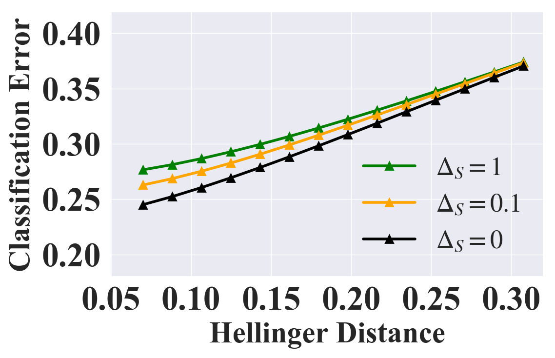
We report the classification error (Error) and BCE loss as the evaluation metric. Figure 1 illustrates the certified fairness on Adult, Compas, Health, and Lawschool under sensitive shifting. More results on two relatively small datasets (Crime, German) are shown in Section E.5. From the results, we see that our certified fairness is tight in practice.
4.2 Certified Fairness with General Shifting
In the general shifting scenario, we similarly randomly generate fair distributions shifted from . Different from sensitive shifting, the distribution conditioned on sensitive attribute and label can also change in this scenario. Therefore, we construct another distribution disjoint with on non-sensitive attributes and mix and in each subpopulation individually guided by mixing parameters satisfying fair base rate constraint. Detailed generation steps are given in Section E.2. Since the fairness certification for general shifting requires bounded loss, we select classification error (Error) and Jensen-Shannon loss (JSD Loss) as the evaluation metric. Figure 2 illustrates the certified fairness with classification error metric under general shifting. Results of JSD loss and more results on two relatively small datasets (Crime, German) are in Section E.5.
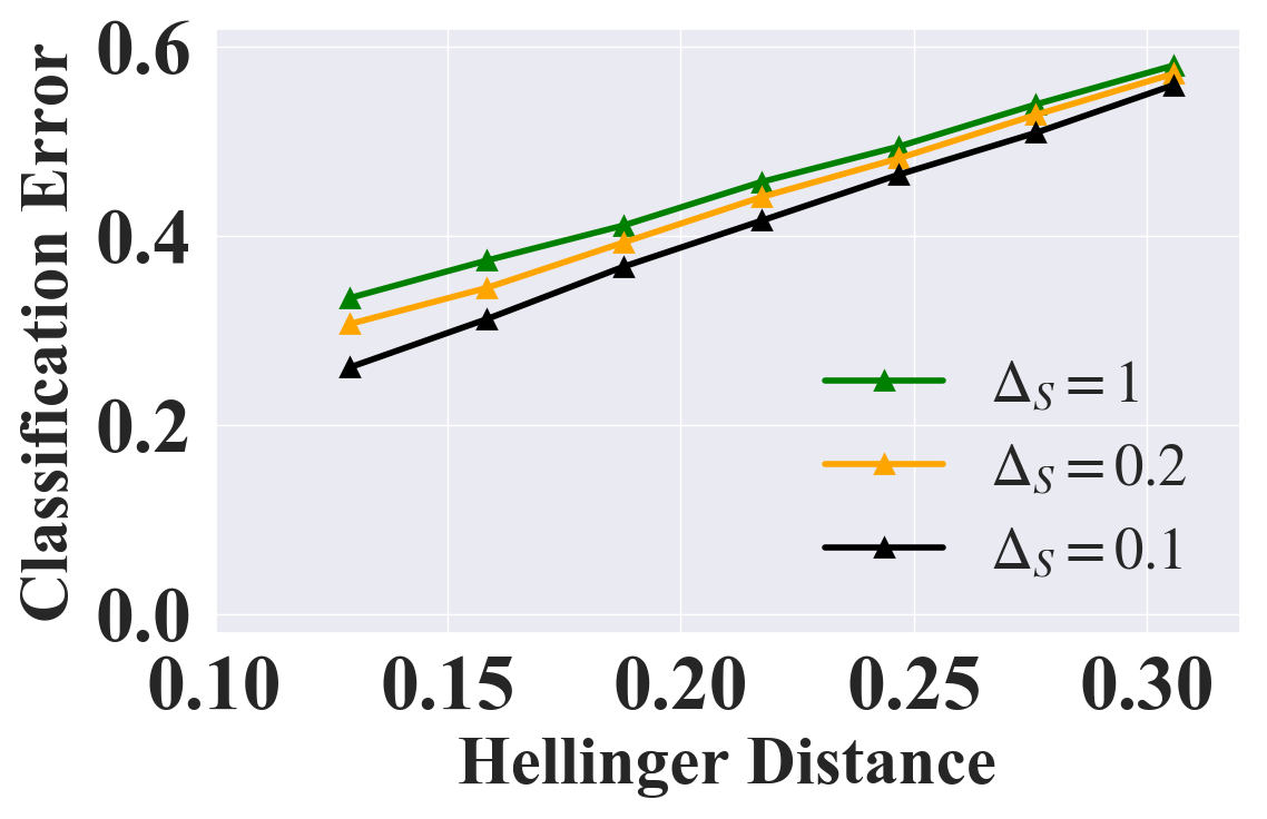
4.3 Certified Fairness with Additional Non-Skewness Constraints
In Section 2.1, we discussed that to represent different real-world scenarios we can add more constraints such as Equation 1 to prevent the skewness of , which can be flexibly incorporated into our certificate framework. Concretely, for sensitive shifting, we only need to add one more box constraint222Note that such modification is only viable when sentive attributes take binary values, which is the typical scenario in the literature of fairness evaluation [39, 38, 31, 42]. where is a parameter controlling the skewness of , which still guarantees convexity. For general shifting, we only need to modify the region partition step2, where we split instead of . The certification results with additional constraints are in Figures 3(a) and 3(b), which suggests that if the added constraints are strict (i.e., smaller ), the bound is tighter. More constraints w.r.t. labels can also be handled by our framework and the corresponding results as well as results on more datasets are in Section E.6.
ADULT

Hellinger Distance
Error
COMPAS

Hellinger Distance
HEALTH

Hellinger Distance
LAW SCHOOL

Hellinger Distance
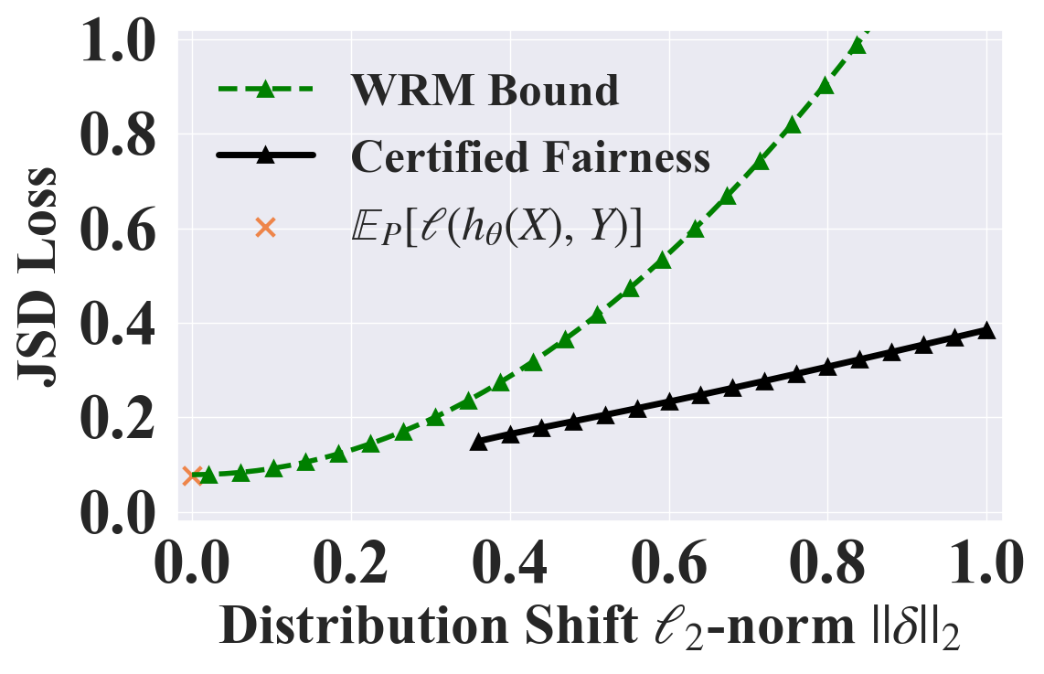
4.4 Comparison with Distributional Robustness Bound
To the best of our knowledge, there is no existing work providing certified fairness on the end-to-end model performance. Thus, we try to compare our bound with the distributional robustness bound since both consider certain distribution shifts. However, it is challenging to directly integrate the fairness constraints into existing bounds. Therefore, we compare with the state-of-the-art distributional robustness certification WRM [43], which solves the similar optimization problem as ours except for the fairness constraint. For fair comparison, we construct a synthetic dataset following [43], on which there is a one-to-one correspondence between the Hellinger and Wasserstein distance used by WRM. We randomly select one dimension as the sensitive attribute. Since WRM has additional assumptions on smoothness of models and losses, we use JSD loss and a small ELU network with 2 hidden layers of size 4 and 2 following their setting. More implementation details are in Section E.4. Results in Figure 3(c) suggest that 1) our certified fairness bound is much tighter than WRM given the additional fairness distribution constraint and our optimization framework; 2) with additional fairness constraint, our certificate problem could be infeasible under very small distribution distances since the fairness constrained distribution does not exist near the skewed original distribution ; 3) with the fairness constraint, we provide non-trivial fairness certification bound even when the distribution shift is large.
5 Conclusion
In this paper, we provide the first fairness certification on end-to-end model performance, based on a fairness constrained distribution which has bounded distribution distance from the training distribution. We show that our fairness certification has strong connections with existing fairness notions such as group parity, and we provide an effective framework to calculate the certification under different scenarios. We provide both theoretical and empirical analysis of our fairness certification.
Acknowledgements.
MK, LL, and BL are partially supported by the NSF grant No.1910100, NSF CNS No.2046726, C3 AI, and the Alfred P. Sloan Foundation. YL is partially supported by the NSF grants IIS-2143895 and IIS-2040800.
References
- [1] Aws Albarghouthi, Loris D’Antoni, Samuel Drews, and Aditya V Nori. Fairsquare: probabilistic verification of program fairness. Proceedings of the ACM on Programming Languages, 1(OOPSLA):1–30, 2017.
- [2] Julia Angwin, Jeff Larson, Surya Mattu, and Lauren Kirchner. Machine bias. In Ethics of Data and Analytics, pages 254–264. Auerbach Publications, 2016.
- [3] Arthur Asuncion and David Newman. Uci machine learning repository, 2007.
- [4] Mislav Balunović, Anian Ruoss, and Martin Vechev. Fair normalizing flows. arXiv preprint arXiv:2106.05937, 2021.
- [5] Solon Barocas and Andrew D Selbst. Big data’s disparate impact. Calif. L. Rev., 104:671, 2016.
- [6] Osbert Bastani, Xin Zhang, and Armando Solar-Lezama. Probabilistic verification of fairness properties via concentration. Proceedings of the ACM on Programming Languages, 3(OOPSLA):1–27, 2019.
- [7] Aharon Ben-Tal, Dick Den Hertog, Anja De Waegenaere, Bertrand Melenberg, and Gijs Rennen. Robust solutions of optimization problems affected by uncertain probabilities. Management Science, 59(2):341–357, 2013.
- [8] Richard Berk, Hoda Heidari, Shahin Jabbari, Michael Kearns, and Aaron Roth. Fairness in criminal justice risk assessments: The state of the art. Sociological Methods & Research, 50(1):3–44, 2021.
- [9] Yatong Chen, Reilly Raab, Jialu Wang, and Yang Liu. Fairness transferability subject to bounded distribution shift. Advances in Neural Information Processing Systems, 2022.
- [10] YooJung Choi, Meihua Dang, and Guy Van den Broeck. Group fairness by probabilistic modeling with latent fair decisions. arXiv preprint arXiv:2009.09031, 2020.
- [11] Alexandra Chouldechova. Fair prediction with disparate impact: A study of bias in recidivism prediction instruments. Big data, 5(2):153–163, 2017.
- [12] Elliot Creager, David Madras, Jörn-Henrik Jacobsen, Marissa Weis, Kevin Swersky, Toniann Pitassi, and Richard Zemel. Flexibly fair representation learning by disentanglement. In International conference on machine learning, pages 1436–1445. PMLR, 2019.
- [13] Amit Datta, Michael Carl Tschantz, and Anupam Datta. Automated experiments on ad privacy settings. Proceedings on privacy enhancing technologies, 2015(1):92–112, 2015.
- [14] John Duchi and Hongseok Namkoong. Variance-based regularization with convex objectives. The Journal of Machine Learning Research, 20(1):2450–2504, 2019.
- [15] John C Duchi, Peter W Glynn, and Hongseok Namkoong. Statistics of robust optimization: A generalized empirical likelihood approach. Mathematics of Operations Research, 2021.
- [16] Harrison Edwards and Amos Storkey. Censoring representations with an adversary. arXiv preprint arXiv:1511.05897, 2015.
- [17] Jeffrey A Gliner. Reviewing qualitative research: Proposed criteria for fairness and rigor. The Occupational Therapy Journal of Research, 14(2):78–92, 1994.
- [18] Moritz Hardt, Eric Price, and Nati Srebro. Equality of opportunity in supervised learning. Advances in neural information processing systems, 29, 2016.
- [19] Kaggle Inc. Heritage health prize kaggle. https://www.kaggle.com/c/hhp, 2022.
- [20] Xisen Jin, Francesco Barbieri, Brendan Kennedy, Aida Mostafazadeh Davani, Leonardo Neves, and Xiang Ren. On transferability of bias mitigation effects in language model fine-tuning. In Proceedings of the 2021 Conference of the North American Chapter of the Association for Computational Linguistics: Human Language Technologies, NAACL-HLT 2021, Online, June 6-11, 2021, pages 3770–3783. Association for Computational Linguistics, 2021.
- [21] Philips George John, Deepak Vijaykeerthy, and Diptikalyan Saha. Verifying individual fairness in machine learning models. In Conference on Uncertainty in Artificial Intelligence, pages 749–758. PMLR, 2020.
- [22] Thomas Kehrenberg, Myles Bartlett, Oliver Thomas, and Novi Quadrianto. Null-sampling for interpretable and fair representations. In European Conference on Computer Vision, pages 565–580. Springer, 2020.
- [23] Jon Kleinberg, Sendhil Mullainathan, and Manish Raghavan. Inherent trade-offs in the fair determination of risk scores. arXiv preprint arXiv:1609.05807, 2016.
- [24] Himabindu Lakkaraju, Jon Kleinberg, Jure Leskovec, Jens Ludwig, and Sendhil Mullainathan. The selective labels problem: Evaluating algorithmic predictions in the presence of unobservables. In Proceedings of the 23rd ACM SIGKDD International Conference on Knowledge Discovery and Data Mining, pages 275–284, 2017.
- [25] Henry Lam. Robust sensitivity analysis for stochastic systems. Mathematics of Operations Research, 41(4):1248–1275, 2016.
- [26] Jiachun Liao, Chong Huang, Peter Kairouz, and Lalitha Sankar. Learning generative adversarial representations (gap) under fairness and censoring constraints. arXiv preprint arXiv:1910.00411, 1, 2019.
- [27] Lydia T Liu, Max Simchowitz, and Moritz Hardt. The implicit fairness criterion of unconstrained learning. In International Conference on Machine Learning, pages 4051–4060. PMLR, 2019.
- [28] Francesco Locatello, Gabriele Abbati, Thomas Rainforth, Stefan Bauer, Bernhard Schölkopf, and Olivier Bachem. On the fairness of disentangled representations. Advances in Neural Information Processing Systems, 32, 2019.
- [29] Christos Louizos, Kevin Swersky, Yujia Li, Max Welling, and Richard Zemel. The variational fair autoencoder. arXiv preprint arXiv:1511.00830, 2015.
- [30] David Madras, Elliot Creager, Toniann Pitassi, and Richard Zemel. Learning adversarially fair and transferable representations. In International Conference on Machine Learning, pages 3384–3393. PMLR, 2018.
- [31] Subha Maity, Debarghya Mukherjee, Mikhail Yurochkin, and Yuekai Sun. Does enforcing fairness mitigate biases caused by subpopulation shift? In M. Ranzato, A. Beygelzimer, Y. Dauphin, P.S. Liang, and J. Wortman Vaughan, editors, Advances in Neural Information Processing Systems, volume 34, pages 25773–25784. Curran Associates, Inc., 2021.
- [32] Andreas Maurer and Massimiliano Pontil. Empirical bernstein bounds and sample variance penalization. arXiv preprint arXiv:0907.3740, 2009.
- [33] Daniel McNamara, Cheng Soon Ong, and Robert C. Williamson. Costs and benefits of fair representation learning. In Proceedings of the 2019 AAAI/ACM Conference on AI, Ethics, and Society, AIES ’19, page 263–270, New York, NY, USA, 2019. Association for Computing Machinery.
- [34] Luca Oneto, Michele Donini, Massimiliano Pontil, and Andreas Maurer. Learning fair and transferable representations with theoretical guarantees. In 2020 IEEE 7th International Conference on Data Science and Advanced Analytics (DSAA), pages 30–39, 2020.
- [35] Adam Paszke, Sam Gross, Francisco Massa, Adam Lerer, James Bradbury, Gregory Chanan, Trevor Killeen, Zeming Lin, Natalia Gimelshein, Luca Antiga, et al. Pytorch: An imperative style, high-performance deep learning library. Advances in neural information processing systems, 32, 2019.
- [36] Momchil Peychev, Anian Ruoss, Mislav Balunović, Maximilian Baader, and Martin Vechev. Latent space smoothing for individually fair representations. arXiv preprint arXiv:2111.13650, 2021.
- [37] Reilly Raab and Yang Liu. Unintended selection: Persistent qualification rate disparities and interventions. Advances in Neural Information Processing Systems, 34, 2021.
- [38] Yuji Roh, Kangwook Lee, Steven Whang, and Changho Suh. Sample selection for fair and robust training. Advances in Neural Information Processing Systems, 34, 2021.
- [39] Anian Ruoss, Mislav Balunovic, Marc Fischer, and Martin Vechev. Learning certified individually fair representations. Advances in Neural Information Processing Systems, 33:7584–7596, 2020.
- [40] Mhd Hasan Sarhan, Nassir Navab, Abouzar Eslami, and Shadi Albarqouni. Fairness by learning orthogonal disentangled representations. In European Conference on Computer Vision, pages 746–761. Springer, 2020.
- [41] Shahar Segal, Yossi Adi, Benny Pinkas, Carsten Baum, Chaya Ganesh, and Joseph Keshet. Fairness in the eyes of the data: Certifying machine-learning models. In Proceedings of the 2021 AAAI/ACM Conference on AI, Ethics, and Society, pages 926–935, 2021.
- [42] Shubhanshu Shekhar, Greg Fields, Mohammad Ghavamzadeh, and Tara Javidi. Adaptive sampling for minimax fair classification. In M. Ranzato, A. Beygelzimer, Y. Dauphin, P.S. Liang, and J. Wortman Vaughan, editors, Advances in Neural Information Processing Systems, volume 34, pages 24535–24544. Curran Associates, Inc., 2021.
- [43] Aman Sinha, Hongseok Namkoong, Riccardo Volpi, and John Duchi. Certifying some distributional robustness with principled adversarial training. arXiv preprint arXiv:1710.10571, 2017.
- [44] Jiaming Song, Pratyusha Kalluri, Aditya Grover, Shengjia Zhao, and Stefano Ermon. Learning controllable fair representations. In The 22nd International Conference on Artificial Intelligence and Statistics, pages 2164–2173. PMLR, 2019.
- [45] Ton Steerneman. On the total variation and hellinger distance between signed measures; an application to product measures. Proceedings of the American Mathematical Society, 88(4):684–688, 1983.
- [46] Caterina Urban, Maria Christakis, Valentin Wüstholz, and Fuyuan Zhang. Perfectly parallel fairness certification of neural networks. Proceedings of the ACM on Programming Languages, 4(OOPSLA):1–30, 2020.
- [47] Maurice Weber, Linyi Li, Boxin Wang, Zhikuan Zhao, Bo Li, and Ce Zhang. Certifying out-of-domain generalization for blackbox functions. In International Conference on Machine Learning. PMLR, 2022.
- [48] Linda F Wightman. Lsac national longitudinal bar passage study. lsac research report series. Law School Admission Council, 1998.
- [49] Robin Winter, Floriane Montanari, Frank Noé, and Djork-Arné Clevert. Learning continuous and data-driven molecular descriptors by translating equivalent chemical representations. Chemical science, 10(6):1692–1701, 2019.
- [50] Samuel Yeom and Matt Fredrikson. Individual fairness revisited: Transferring techniques from adversarial robustness. arXiv preprint arXiv:2002.07738, 2020.
- [51] Rich Zemel, Yu Wu, Kevin Swersky, Toni Pitassi, and Cynthia Dwork. Learning fair representations. In International conference on machine learning, pages 325–333. PMLR, 2013.
- [52] Xueru Zhang, Ruibo Tu, Yang Liu, Mingyan Liu, Hedvig Kjellstrom, Kun Zhang, and Cheng Zhang. How do fair decisions fare in long-term qualification? Advances in Neural Information Processing Systems, 33:18457–18469, 2020.
- [53] Han Zhao, Amanda Coston, Tameem Adel, and Geoffrey J Gordon. Conditional learning of fair representations. arXiv preprint arXiv:1910.07162, 2019.
- [54] Han Zhao and Geoff Gordon. Inherent tradeoffs in learning fair representations. Advances in neural information processing systems, 32, 2019.
Appendices
Contents
Appendix A Broader Impact
This paper aims to calculate a fairness certificate under some distributional fairness constraints on the performance of an end-to-end ML model. We believe that the rigorous fairness certificates provided by our framework will significantly benefit and advance social fairness in the era of deep learning. Especially, such fairness certificate can be directly used to measure the fairness of an ML model regardless the target domain, which means that it will measure the unique property of the model itself with theoretical guarantees, and thus help people understand the risks of existing ML models. As a result, the ML community may develop ML training algorithms that explicitly reduce the fairness risks by regularizing on this fairness certificate.
A possible negative societal impact may stem from the misunderstanding or inaccurate interpretation of our fairness certificate. As a first step towards distributional fairness certification, we define the fairness through the lens of worst-case performance loss on a fairness constrained distribution. This fairness definition may not explicitly imply an absoluate fairness guarantee under some other criterion. For example, it does not imply that for any possible individual input, the ML model will give fair prediction. We tried our best in Section 2 to define the certification goal, and the practitioners may need to understand this goal well to avoid misinterpretation or misuse of our fairness certification.
Appendix B Omitted Background
We illustrate omitted background in this appendix.
B.1 Hellinger Distance
As illustrated in the beginning of Section 3, our framework uses Hellinger distance to bound the distributional distance. A formal definition of Hellinger distance is as below.
Definition 3 (Hellinger Distance).
Let and be distributions on that are absolutely continuous with respect to a reference measure with . The Hellinger distance between and is defined as
| (10) |
where and are the Radon-Nikodym derivatives of and with respect to , respectively. The Hellinger distance is independent of the choice of the reference measure .
Representative properties for the Hellinger distance are discussed in Section 3.
B.2 Thm. 2.2 in [47]
As mentioned in Section 3.3, we leverage Thm. 2.2 from [47] to upper bound the expected loss of in each shifted subpopulation . Here we restate Thm. 2.2 for completeness.
Theorem 4 (Thm. 2.2, [47]).
Let and denote two distributions supported on , suppose that , then
| (11) | ||||
where , for any given distance bound that satisfies
| (12) |
This theorem provides a closed-form expression that upper bounds the mean loss of on shifted distribution (namely ), given bounded Hellinger distance and the mean and variance of loss on under two mild conditions: (1) the function is positive and bounded (denote the upper bound by ); and (2) the distance is not too large (specifically, ). Since Equation 12 holds for arbitrary models and loss functions as long as the function value is bounded by , using Equation 12 allows us to provide a generic and succinct fairness certificate in Thm. 3 for general shifting case that holds for generic models including DNNs without engaging complex model architectures. Indeed, we only need to query the mean and variance under for the given model to compute the certificate in Equation 12, and this benefit is also inherited by our certification framework expressed by Thm. 3. Note that there is no tightness guarantee for this bound yet, which is also inherited by our Thm. 3.
Appendix C Proofs of Main Results
This appendix entails the complete proofs for Proposition 1, Thm. 1, Thm. 2, Equation 6, and Thm. 3 in the main text. For complex proofs such as that for Thm. 3, we also provide high-level illustration before going into the formal proof.
C.1 Proof of Proposition 1
Proof of Proposition 1.
Since each term is within , we consider two cases: and . If , and so will be their differences for and . If , , and also the differences for and are always within . This proves -EO.
Now consider DP. We notice that for any ,
| (13) |
Thus,
which proves -DP, where leverages the fair base rate property of which gives .
∎
C.2 Proof of Thm. 1
Proof of Thm. 1.
We first prove the key eq. 3.
| (14) |
where and are density functions of subpopulation distributions and respectively.
Then, we show that any feasible solution of Equation 2 satisfies the constraints in Equation 4. We let and denote a feasible solution of Equation 2, i.e.,
| (15) |
We let denote the proportions of within each support partition , and the in each subpopulation. By Equation 14, we have where . Note that by definition, and . Furthermore, by the implication relations stated in Thm. 1, for any , ; and for any , . To this point, we have shown and satisfy all constraints in Equation 4, i.e., and is a feasible solution of Equation 4. Since Equation 4 expresses the optimal (maximum) solution, Equation 4 (in Thm. 1) Equation 2. ∎
C.3 Proof of Thm. 2
Proof of Thm. 2.
The proof of Thm. 2 is composed of three parts: (1) the optimization problem provides a fairness certificate for Problem 2; (2) the certificate is tight; and (3) the optimization problem is convex.
-
(1)
Suppose the maximum of Problem 2 is attained with the test distribution in the sensitive shifting setting, then we decompose both and according to both the sensitive attribute and the label:
(16) Since is a fair base rate distribution, for any , where . As a result, . Now we define
(17) and then
(18) By the distance constraint in Problem 2 (namely ) and Equation 14, we have
(19) Since there is only sensitive shifting, , given Equation 18, we have
(20) Now, we can observe that the and induced by satisfy all constraints of Problem 2. For the objective,
Objective in Thm. 2 (by Equation 18 and ) Therefore, the optimal value of Thm. 2 will be larger or equal to the optimal value of Problem 2 which concludes the proof of the first part.
-
(2)
Suppose the optimal value of Thm. 2 is attained with and . We then construct . We now inspect each constraint of Problem 2. The constraint is satisfied because is satisfied as a constraint of Thm. 2. Apparently, . Then, is a fair base rate distribution because
(21) is a constant across all . Thus, satisfies all constraints of Problem 2 and
Optimal objective of Problem 2 (22) Combining with the conclusion of the first part, we know optimal values of Thm. 2 and Problem 2 match, i.e., the certificate is tight.
-
(3)
Inspecting the problem definition in Thm. 2, we find the objective and all constraints but the last one are linear. Therefore, to prove the convexity of the optimization problem, we only need to show that the last constraint
(23) is convex with respect to and . Given two arbitrary feasible pairs of and satisfying Equation 23, namely and , we only need to show that also satisfies Equation 23, where , . Indeed,
(Cauchy’s inequality)
∎
C.4 Proof of Equation 6
Proof of Equation 6.
The proof of Equation 6 is composed of two parts: (1) the optimization problem provides a fairness certificate for Problem 1; and (2) the certificate is tight. The high-level proof sketch is similar to the proof of Thm. 2.
-
(1)
Suppose that the maximum of Problem 1 is attained with the test distribution under the general shifting setting, then we decompose both and according to both the sensitive attribute and the label:
(24) Unlike sensitive shifting setting, in general shifting setting, here the subpopulation of is instead of due to the existence of distribution shifting within each subpopulation.
Following the same argument as in the first part proof of Thm. 2, since is a fair base rate distribution, we can define
(25) and write
(26) since . We also define . Now we show these along with model parameter constitute a feasible point of Equation 6, and the objectives of Equation 6 and Problem 2 are the same given .
-
•
(Feasibility)
There are three constraints in Equation 6. By the definition of and , naturally Equation 6b is satisfied. Then, according to Equation 14 and the definifition of above, Equation 6c and Equation 6d are satisfied. -
•
(Objective Equality)
Equation 6a (27)
As a result, the optimal value of Equation 6 is larger than or equal to the optimal value of Problem 1, and hence the optimization problem encoded by Equation 6 provides a fairness certificate.
-
•
-
(2)
To prove the tightness of the certificate, we only need to show that the optimal value of the optimization problem in Equation 6 is also attainable by the original Problem 1.
Suppose that the optimal objective of Equation 6 is achieved by optimizable parameters , and . Then, we construct . We first show that is a feasible point of Problem 1, and then show that the objective given is equal to the optimal objective of Equation 6.
-
•
(Feasibility)
There are two constraints in Problem 1: the bounded distance constraint and the fair base rate constraint. The bounded distance constraint is satisfied due to applying Equation 14 along with Equations 6c and 6d. The fair base rate constraint is satisfied following the same deduction as in Equation 21. -
•
(Objective Equality)
Objective Problem 1
Thus, the optimal value of the optimization problem in Equation 6 is attainable also by the original Problem 1 which concludes the tightness proof.
-
•
∎
C.5 Proof of Thm. 3
High-Level Illustration.
The starting point of our proof is Equation 6, where we have shown a fairness certificate for Problem 1 (general shifting setting). Then, we plug in Thm. 2.2 in [47] (stated as Equation 12 in Section B.2) to upper bound the expected loss within each sub-population. Now, we get an optimization problem involving , , and that upper bounds the optimization problem in Equation 6. In this optimization problem, we find and are bounded in , and once these two variables are fixed, the optimization with respect to becomes convex. Using this observation, we propose to partition the feasible space of and into sub-regions and solve the convex optimization within each region bearing some degree relaxation, which yields Thm. 3.
Proof of Thm. 3.
The proof is done stage-wise: starting from Equation 6, we apply relaxation and derive a subsequent optimization problem that upper bounds the previous one stage by stage, until we get the final expression in Thm. 3.
To demonstrate the proof, we first define the optimization problems at each stage, then prove the relaxations between each adjacent stage, and finally show that the last optimization problem contains a finite number of ’s values where each is a convex optimization, so that the final optimization problem provides a computable fairness certificate.
We define these quantities, for :
| (28) | ||||
Given and the above quantities, the optimization problem definitions are:
-
•
(29a) (29b) (29c) (29d) -
•
After applying Equation 12:
(30a) (30b) (30c) (30d) -
•
After variable transform :
(31a) (31b) (31c) (31d) -
•
After feasible region partitioning on and :
(32a) (32b) (32c) (32d) (32e) -
•
Final quantity in Thm. 3:
(33a) (33b) (33c) (33d) (33e)
We have this relation:
| (34) |
Thus, when and , given that is a non-negative loss by Section 2, we can see Equation 33, i.e., the expression in Thm. 3’s statement, upper bounds Problem 1, i.e., provides a fairness certificate for Problem 1. The proofs of these equalities/inequalities are in the following parts labeled by (A), (B), (C), and (D) respectively.
Now we show that each queried by Equation 7 (or equally Equation 33a) is a convex optimization. Inspecting ’s objective, with respect to the optimizable variable , we find that the only non-linear term in the objective is . Consider the function . Define and , and then . Thus, and . Notice that , , and for . Thus, . Since is twice differentiable in , we can conclude that is concave and so does the objective of Equation 7. Inspecting ’s constraints, we observe that the only non-linear constraint is . Due to the concavity of function , we have for any two feasible points and . Thus, this non-linear constraint defines a convex region. To this point, we have shown that ’s objective is concave and ’s constraints are convex, given that is a maximization problem, is a convex optimization. ∎
Under the assumptions that and :
-
(A)
Proof of Equation 29 Equation 30.
Given Equation 29d, for each , applying Equation 12, we get(35) Plugging this inequality into all in Equation 29a, we obtain Equation 30. ∎
-
(B)
Proof of Equation 30 Equation 31.
By Equation 30d, . Therefore, is a one-to-one mapping, and we can use to parameterize , which yields Equation 31. ∎ -
(C)
Proof of Equation 31 Equation 32.
From Equation 31b, we notice that the feasible range of and is subsumed by . We now partition this region for each variable to sub-regions: , , and then consider the maximum value across all the combinations of each sub-region for variables and , when feasible. As a result, Equation 31 can be written as the maximum over all such sub-problems where ’s and ’s enumerate all possible sub-region combinations, which is exactly encoded by Equation 32. ∎ -
(D)
Proof of Equation 32 Equation 33.
We only need to show that when is feasible,(36) Since both and are maximization problem, we only need to show that the objective of upper bounds that of , and the constraints of are equal or relaxations of those of .
For the objective, given that and , for any , We observe that
(37) and by summing up all these terms for all and , the LHS would be the objective of and the RHS would be the objective of . Hence, ’s objective upper bounds that of .
For the constraints, similarly, given that and , we have
(32e) which implies that all feasible solutions of are also feasible for . Combining with the fact that for any solution of , its objective value is greater than or equal to that of as shown above, we have Equation 36 which concludes the proof. ∎
Appendix D Omitted Theorem Statements and Proofs for Finite Sampling Error
D.1 Finite Sampling Confidence Intervals
Lemma D.1.
Let be set of i.i.d. finite samples from , and let for any . Let be a loss function. We define , , and . Then for , with respect to the random draw of from , we have
| (38) | |||
| (39) | |||
| (40) |
Proof of Lemma D.1.
We can get Equation 39 according to Theorem 10 in [32]. Here, we will provide proofs for Equation 38 and Equation 40, respectively. The general idea is to use Hoeffding’s inequality to get the high-confidence interval.
We will prove Equation 38 first. From Hoeffding’s inequality, for all , we have:
| (41) |
Since we want to get an interval with confidence , we let , from which we can derive that
| (42) |
Plugging Equation 42 into Equation 41, we can get:
| (43) |
Then we will prove Equation 40. From Hoeffding’s inequality, for all , we have:
| (44) |
Since we want to get an interval with confidence , we let , from which we can derive that
| (45) |
Plugging Equation 45 into Equation 44, we can get:
| (46) |
∎
D.2 Fairness Certification Statements with Finite Sampling
Theorem 5 (Thm. 2 with finite sampling).
Theorem 6.
If for any and , and , given a distance bound and any , for any region granularity , the following expression provides a fairness certificate for Problem 1 with probability at least :
| (48) |
| (49a) | ||||
| (49b) | ||||
| (49c) | ||||
| (49d) | ||||
where , ; , , , , , computed with Lemma D.1, and , , . Equation 48 only takes ’s value when it is feasible, and each queried by Equation 48 is a convex optimization.
D.3 Proofs of Fairness Certification with Finite Sampling
High-Level Illustration.
We use Hoeffding’s inequality to bound the finite sampling error of statistics and add the high confidence box constraints to the optimization problems, which can still be proved to be convex.
Proof of Thm. 5.
The proof of Thm. 5 is composed of two parts: (1) the optimization problem provides a fairness certificate for Problem 2; (2) the optimization problem is convex.
-
(1)
We prove that Thm. 5 provides a fairness certificate for Problem 2 in this part. Since Thm. 2 provides a fairness certificate for Problem 2, we only need to prove: (a) the feasible region of the optimization problem in Thm. 2 is a subset of the feasible region of the optimization problem in Thm. 5, and (b) the optimization objective in Thm. 2 can be upper bounded by that in Thm. 5.
To prove (a), we first equivalently transform the optimization problem in Thm. 2 into the following optimization problem by adding to the decision variables:
(50a) (50b) (50c) (50d) (50e) For decision variables and , optimization 47 and 50 has the same constraints (Equation 47b and Equation 50b). For decision variables , the feasible region of in optimization 47 (decided by Equations 47d and 47e) is a subset of the feasible region of in optimization 50 (decided by Equations 50d and 50e), since . Therefore, the feasible region with respect to , , and of the optimization problem in Thm. 2 is a subset of that in Thm. 5.
To prove (b), we only need to show that the objective in Equation 47a can be upper bounded by the objective in Equation 50a. The statement consistently holds because and .
-
(2)
Inspecting that the objective and all the constraints in optimization problem in Equation 47 are linear with respect to , , but the one in Equation 47c. Therefore, we only need to prove that the following constraint is convex with respect to , , :
(51) We define a function with respect to vector : . Then we can derive that:
(52) Therefore, the function is convex with respect to . Similarly, we can prove the convexity with respect to and . Finally, we can conclude that the constraint in Equation 51 is convex with respect to , , and the optimization problem defined in Thm. 5 is convex.
Since we use the union bound to bound and for all simultaneously, the confidence is . ∎
Proof of Thm. 6.
The proof of Thm. 6 includes two parts: (1) the optimization problem provides a fairness certificate for Problem 1; (2) each queried by Equation 48 is a convex optimization.
-
(1)
Since Thm. 3 provides a fairness certificate for Problem 1, we only need to prove: (a) the feasible region of the optimization problem in Thm. 3 is a subset of that in Thm. 6, and (b) the optimization objective in Thm. 3 can be upper bounded by that in Thm. 6.
To prove (a), we first equivalently transform the optimization problem in Thm. 3 into the following optimization problem by adding to the decision variables:
(53a) (53b) (53c) (53d) (53e) For decision varibales , since and , the feasible region of in Equation 53 is a subset of that in Equation 49. For decision variables , since , the feasible region of in Equation 53 is also a subset of that in Equation 49. Therefore, the feasible region of the optimization problem in Thm. 3 is a subset of that in Thm. 6.
To prove (b), we only need to show that the objective in Equation 53a can be upper bounded by the objective in Equation 49a. Since and hold, we can observe that ,
-
(2)
We will prove that each queried by Equation 48 is a convex optimization with respect to decision variables and in this part. In the proof of Thm. 3, we provide the proof of convexity with respect to , so we only need to prove that the optimization problem is convex with respect to . We can observe that the constraints of in Equation 49d is linear, and thus we only need to prove that (the constraint in Equation 49c) is convex with respect to . Here, we define a function with respect to vector : . Then we can derive that:
(55) Thus, the function is convex and defines a convex set with respect to . Then, we prove that the constraint is convex with respect to .
Since we use the union bound to bound , and for all simultaneously, the confidence is . ∎
Appendix E Experiments
E.1 Datasets
We validate our certified fairness on six real-world datasets: Adult [3], Compas [2], Health [19], Lawschool [48], Crime [3], and German [3]. All the used datasets contain categorical data.
In Adult dataset, we have 14 attributes of a person as input and try to predict whether the income of the person is over k $/year. The sensitive attribute in Adult is selected as the sex.
In Compas dataset, given the attributes of a criminal defendent, the task is to predict whether he/she will re-offend in two years. The sensitive attribute in Compas is selected as the race.
In Health dataset, given the physician records and and insurance claims of the patients, we try to predict ten-year mortality by binarizing the Charlson Index, taking the median value as a cutoff. The sensitive attribute in Health is selected as the age.
In Lawschool dataset, we try to predict whether a student passes the exam according to the appication records of different law schools. The sensitive attribute in Lawschool is the race.
In Crime dataset, we try to predict whether a specific community is above or below the median number of violent crimes per population. The sensitive attribute in Crime is selected as the race.
In German dataset, each person is classified as good or bad credit risks according to the set of attributes. The sensitive attribute in German is selected as the sex.
Following [39], we consider the scenario where sensitive attributes and labels take binary values, and we also follow their standard data processing steps: (1) normalize the numerical values of all attributes with the mean value 0 and variance 1, (2) use one-hot encodings to represent categorical attributes, (3) drop instances and attributes with missing values, and (4) split the datasets into training set, validation set, and test set.
Training Details. We directly train a ReLU network composed of two hidden layers on the training set of six datasets respectively following the setting in [39]. Concretely, we train the models for 100 epochs with a batch size of 256. We adopt the binary cross-entropy loss and use the Adam optimizer with weight decay 0.01 and dynamic learning rate scheduling (ReduceLROnPlateau in [35]) based on the loss on the validation set starting at 0.01 with the patience of 5 epochs.
E.2 Fair Base Rate Distribution Generation Protocol
To evaluate how well our certificates capture the fairness risk in practice, we compare our certification bound with the empirical loss evaluated on randomly generated fairness constrained distributions shifted from . Now, we introduce the protocols to generate fairness distributions for sensitive shifting and general shifting, respectively. Note that the protocols are only valid when the sensitive attributes and labels take binary values.
Fair base rate distributions generation steps in the sensitive shifting scenario:
-
(1)
Sample the proportions of subpopulations of the generated distribution : uniformly sample two real values in the interval , and do the assignment: , , , .
-
(2)
Determine the sample size of every subpopulation: first determine the subpopulation which requires the largest sample size, use all the samples in that subpopulation, and then calculate the sample size in other subpopulations according to the proportions.
-
(3)
Uniformly sample in each subpopulation based on the sample size.
-
(4)
Calculate the Hellinger distance . Suppose that the support of and is and the densities of and with respect to a suitable measure are and , respectively. Since we consider sensitive shifting here, we have where is a scalor. The derivation of the distance calculation formula is shown as follows,
(56a) (56b) (56c) (56d) (56e)
Fair base rate distribution generation steps in the general shifting scenario:
-
(1)
Construct a data distribution that is disjoint with the training data distribution by changing the distribution of non-sensitive values given the sensitive attributes and labels.
-
(2)
Sample mixing parameters and in the interval satisfying (base rate parity) and .
-
(3)
Determine the proportion of every subpopulation in distribution : .
-
(4)
Determine the sample size of every subpopulation in and : first determine the subpopulation which requires the largest sample size, use all the samples in that subpopulation, and then calculate the sample size in other subpopulations according to the proportions.
-
(5)
Calculate the Hellinger distance between distribution and : . Suppose that the support of and is and the densities of and with respect to a suitable measure are and , respectively. The derivation of the distance calculation formula is shown as follows,
(57a) (57b) (57c) (57d) (57e)
E.3 Implementation Details of Our Fairness Certification
We conduct vanilla training and then calculate our certified fairness according to our certification framework. Concretely, in the training step, we train a ReLU network composed of 2 hidden layers of size 20 for 100 epochs with binary cross entropy loss (BCE loss) using an Adam optimizer. The initial learning rate is 0.05 for Crime and German datasets, while for other datasets, the initial learning rate is set . We reduce the learning rate with a factor of 0.5 on the plateau measured by the loss on the validation set with patience of 5 epochs. In the fairness certification step, we set the region granularity to be for certification in the general shifting scenario. We use confidence interval when considering finite sampling error. The codes we used follow the MIT license. All experiments are conducted on a 1080 Ti GPU with 11,178 MB memory.
E.4 Implementation Details of WRM
The optimization problem of tackling distributional robustness is formulated as:
| (58) |
where is a predetermined distribution distance metric. Note that the optimization is the same as our certified fairness optimization in Problem 1 except for the fairness constraint.
WRM [43] proposes to use the dual reformulation of the Wasserstein worst-case risk to provide the distributional robustness certificate, which is formulated in the following proposition.
Proposition 2 ([43], Proposition 1).
Let and be continuous and let . Then, for any distribution and any ,
| (59) |
where is the 1-Wasserstein distance between and .
One requirement for the certificate to be tractable is that the surrogate function is concave with respect to , which holds when is larger than the Lipschitz constant of the gradient of with respect to . Since we use the ELU network with JSD loss, we can efficiently calculate iteratively as shown in Appendix D of [47].
We select Gaussian mixture data for fair comparison. The Gaussian mixture data can be formulated as where is the number of Gaussian data, is the proportion of the -th Gaussian, and . In our evaluation, we use 2-dimension Gaussian and mixture data composed of 2 Gaussian () labeled and , respectively. Concretely, we let and . The second dimension of input vector is selected as the sensitive attribute , and the base rate constraint becomes: . Given the perturbation that induces , the Wasserstein distance and Hellinger distance can be formulated as follows:
| (60) |
E.5 More Results of Certified Fairness with Sensitive Shifting and General shifting
CRIME

Classification Error
GERMAN


Hellinger Distance
BCE Loss

Hellinger Distance
CRIME

Classification Error
GERMAN


Hellinger Distance
JSD Loss

Hellinger Distance
ADULT

Hellinger Distance
JSD Loss
COMPAS

Hellinger Distance
HEALTH

Hellinger Distance
JSD Loss
LAW SCHOOL

Hellinger Distance
E.6 More Results of Certified Fairness with Additional Non-Skewness Constraints


E.7 Fair Classifier Achieves High Certified Fairness
We compare the fairness certificate of the vanilla model and the perfectly fair model on Adult dataset to demonstrate that our defined certified fairness in Problem 1 and Problem 2 can indicate the fairness in realistic scenarios. In Adult dataset, we have 14 attributes of a person as input and try to predict whether the income of the person is over k $/year. The sensitive attribute in Adult is selected as the sex. We consider four subpopulations in the scenario: 1) male with salary below k, 2) male with salary above k, 3) female with salary below k, and 4) female with salary above k. We take the overall 0-1 error as the loss. The vanilla model is real, and trained with standard training loss on the Adault dataset. The perfectly fair model is hypothetical and simulated by enforcing the loss within each subpopulation to be the same as the vanilla trained classifier’s overall expected loss for fair comparison with the vanilla model. From the experiment results in Table 1 and Table 2, we observe that our fairness certificates correlate with the actual fairness level of the model and verify that our certificates can be used as model’s fairness indicator: the certified fairness of perfectly fair models are consistently higher than those for the unfair model, for both the general shifting scenario and the sensitive shifting scenario. These findings demonstrate the practicality of our fairness certification.
| Hellinger Distance | 0.1 | 0.2 | 0.3 | 0.4 | 0.5 |
|---|---|---|---|---|---|
| Vanilla Model Fairness Certificate | 0.182 | 0.243 | 0.297 | 0.349 | 0.397 |
| Fair Model Fairness Certificate | 0.148 | 0.148 | 0.148 | 0.148 | 0.148 |
| Hellinger Distance | 0.1 | 0.2 | 0.3 | 0.4 | 0.5 |
|---|---|---|---|---|---|
| Vanilla Model Fairness Certificate | 0.274 | 0.414 | 0.559 | 0.701 | 0.828 |
| Fair Model Fairness Certificate | 0.266 | 0.407 | 0.553 | 0.695 | 0.824 |