Centrality-Weighted Opinion Dynamics:
Disagreement and Social Network Partition
Abstract
This paper proposes a network model of opinion dynamics based on both the social network structure and network centralities. The conceptual novelty in this model is that the opinion of each individual is weighted by the associated network centrality in characterizing the opinion spread on social networks. Following a degree-centrality-weighted opinion dynamics model, we provide an algorithm to partition nodes of any graph into two and multiple clusters based on opinion disagreements. Furthermore, the partition algorithm is applied to real-world social networks including the Zachary karate club network [1] and the southern woman network [2] and these application examples indirectly verify the effectiveness of the degree-centrality-weighted opinion dynamics model. Finally, properties of general centrality-weighted opinion dynamics model are established.
I Introduction
I-A Motivation and background
Posts on online social platforms, opinions of individuals in social networks, or ideas in research papers, tend to be weighted (or perceived) differently due to the heterogeneity of hyperlink networks, social connections, or citation structures. These differences may be influenced by the ranking in Google search, social importance in social networks, or citation counts in citation networks. Network centralities, which quantify how central nodes are in a network, play a natural role in the phenomenon of heterogeneous weights (in posts, opinions or ideas) in these examples above. In particular, centrality weights proportional to nodal connection degrees may appear naturally in networks (see for example the preferential attachment network-growth model [3] for scale-free networks). Network influence weighted by connection degrees may well represent an underlying natural principle in the evolution of opinions and influences on social networks.
The modelling of opinion dynamics dates back to the work of French [4] via agent-based models on directed graphs, the work of Degroot [5] based on Markov process and that of Friedkin and Johnsen [6] based on dynamical systems. There have been many useful variations based on these basic models (see for instance [7, 8, 9, 10, 11, 12] and the references therein for an overview). The study of opinion dynamics [4, 5, 6] connects inherently to the study of distributed coordination or the consensus protocol (see for instance [13, 14, 15]), which employs locally the relative state differences among neighbours. In this type of modelling, it is typically assumed that the “influence matrix” or “influence network” is given beforehand. However the influence matrix is not necessarily the social network structure and to the best knowledge of the author, there lacks a systematic way of identifying the influence matrix from network structures in the study of opinion dynamics. A second type of models to study the mechanism of opinion evolution and decision-making on a social network is via the Ising model with state-dependent network interactions [16], and the large-scale network opinion analysis is based on statistical characterizations of the underlying opinions [17, 18]. For this type of models, it is quite difficult to obtain explicit solutions and one typically needs to rely on numerical simulations or mean-field approximations [16, 17, 18]. In addition, plenty of research papers have approached the modelling of opinion evolution from Bayesian update perspectives (see for instance, [19, 20, 21, 22]). Readers are referred to [7, 12] for an overview of the extensive research in modelling opinion dynamics. In the current paper, the basic model of studying opinion dynamics over networks is based on [5, 6]
Centralities have been employed in modelling opinion dynamics in various different ways. The work [23] studied the opinion formation problem by incorporating the Ising model with the page-rank centrality [24]. The paper [25] provided a dynamics update model based on Erdös-Rényi random graphs and centralities such as in-degree, closeness and page-rank centralities. A centrality notion as the asymptotic opinion state was studied in [10]. These papers, among others, are different from the current paper in both the model formulation and the use of centralities in modelling opinion dynamics.
Social choice problems based on network structures are essentially graph partition problems, which have been studied from various perspectives (see for instance [26, 27, 28, 29, 30]). Such problems also arise from image segmentation (see for instance [31] the references therein). Various approaches, such as minimal spanning tree methods [31], spectral partition [26, 28], modularity matrix approach [32, 29], have been used to solve graph partition problems (see [31, 33] for a survey of different methods). In particular, spectral partition forms an important heuristic method for partitioning graphs [28]. The study of graph spectral partition method started in 1970s in [34, 35] based on eigenvectors of adjacency matrices and in [36, 37] based on the Fielder eigenvector (i.e., the eigenvector associated with the smallest non-zero eigenvalue of the graph Laplacian). In this paper, a spectral partition based on the centrality-weighted network provides us an algorithm to partition social networks.
I-B Contribution
We propose a simple and concrete procedure to build “influence networks” based on social network structures and network centralities for the modelling of opinion dynamics. Then following a degree-centrality-weighted opinion dynamics, we provide a method for network partitions based on the disagreements approximately represented by the projection of the opinion state in the most significant eigendirection that is orthogonal to agreement subspace. This partition method produces the exact result for the split of the Zachary’s karate club network [1], which indirectly verifies the effectiveness of our degree-centrality-weighted opinion dynamics model. Compared to network partition algorithm in [29] based on modularity measure which also correctly characterizes the partition for the Zachary’s karate club network [1], our method provides a different theoretical interpretation of the network partition based on the disagreement of opinions from a dynamical system point of view, and this explanation fits naturally into the context of the social choice problem in [1].
Notation and terminology
Let . Let represent the diagonal matrix with the diagonal elements specified by the vector . (resp. ) denotes the diagonal matrix with diagonal elements given by (resp. ). denotes the -dimensional column vector with all elements being one. For any matrix , to denote its transpose.
A square matrix is diagonalizable if there exist an invertible real matrix and a diagonal real matrix such that . An eigenvalue of a matrix is defined as the complex or real number such that there exists a complex or real vector satisfying . Then is called an eigenvector of associated with the eigenvalue . Let denote the identity matrix with an appropriate dimension. Then the algebraic multiplicity of an eigenvalue of is defined as the multiplicity of as a root of ; the geometric multiplicity of an eigenvalue is defined as the maximum number of linearly independent eigenvectors associated with , which can be computed by when is of dimension . In this paper, whenever we list the eigenvalues of a matrix, we always order the eigenvalues in a non-decreasing order, that is,
A graph is defined by the set of nodes and the set of edges connecting the nodes. A weighted graph is a graph in which each edge is associated with a real number weight. Taking the node set , then a graph can be represented by its adjacency matrix where denotes the weight from node to node . A graph is undirected if the connection weight from to is always equal to the weights from to for all (that is, its adjacency matrix satisfies ). denotes the graph with as the adjacency matrix and as the node set. denotes the (incoming) neighborhood of node . A path (resp. directed path) from node to is defined as a finite or infinite sequence of edges which joins a sequence of distinct nodes (resp. and the directed edges are in the same direction). An undirected graph is connected if for every node pair on the graph one can identify a path. A directed graph is strongly connected if every node pair on the graph has a directed path from to .
II Opinion evolution over social networks
II-A Degree-centrality-weighted opinion dynamics
Social conformity characterizes the phenomenon that individuals tends to change his/her behavior or response to conform with that of the group and it has supporting evidence in social and psychology studies (see for instance [38]). Considering social conformity, basic assumptions in our degree-centrality-weighted opinion dynamics model are as follows:
-
(i)
Individuals on a social network communicate and change their own opinions in the direction to conform with those of their neighbours;
-
(ii)
Each individual weights these influences from the neighbours based on their importance on the network in terms of the number of their connections.
Based on these basic assumptions, the dynamics for opinion evolution over a social network are then formulated as follows:
| (1) |
where is the degree (centrality) of node on the network, is social connection weight between nodes and (which can take a real value if the underlying social network is weighted, or 0-1 value if the underlying graph only characterizes the social network structure), and is a fixed time constant.
Let denote the adjacency matrix of the underlying graph. The degree centrality vector is given by Then the “influence matrix” for (1) is given by
Clearly is not necessarily symmetric. The corresponding Laplacian matrix of this weighted “influence matrix” is then given by
where the last equality holds because
| (2) |
We note that the Laplacian matrix is different from normalized Laplacian matrices (by connection degrees) of which are typically given by
Denote . Then the dynamics in (1) have the following compact representation
| (3) |
where the Laplacian matrix and the adjacency matrix are respectively given by
II-B Properties of the influence matrix and its Laplacian
Proposition 1 (Appendix -A)
If the underlying graph with the adjacency matrix is connected and undirected, then the Laplacian matrix contains only one zero eigenvalue and all the other eigenvalues of have strictly positive real parts. □
If the underlying graph with the adjacency matrix is connected and undirected, then Proposition 1 implies that the long-term behaviour of the system model (3) reaches agreement as follows where is the normalized right eigenvector of and is the normalized left eigenvector of that associated with the only zero eigenvalue . (See for instance [39]).
Proposition 2 (Appendix -B)
If the underlying graph with the adjacency matrix is connected and undirected, then all the eigenvalues of and are real. □
The conclusion in Proposition 2 on real eigenvalues for and may not hold when is not a symmetric matrix.
Proposition 3 (Appendix -C)
If the underlying graph with the adjacency matrix is connected and undirected, then and are diagonalizable. □
Henceforth we assume that with the adjacency matrix is undirected and connected. Based on Proposition 3, is diagonalizable, and hence the solution to (1) is explicit given by
| (4) |
where and represent respectively the left and right orthonormal eigenvectors of associated with eigenvalue (allowing repeated eigenvalues), .
II-C Network opinion partition algorithm
The disagreement state is defined as the state projection into the subspace that is orthogonal to the agreement subspace (which is equivalently ) in the opinion state space. Then the disagreement state of (4) is given by
| (5) |
The disagreement state converges to the origin exponentially over time and the slowest rate is governed by the smallest non-zero eigenvalue of . Hence to approximately characterize the disagreement over networks, one may use the smallest non-zero eigenvalues and its associated left and right eigenvectors.
The basic idea for the partition algorithm is then to analyze the opinion state projected into the subspace associated with the eigenvector(s) of . The signs of this projected opinion state will cluster nodes into two groups.
Partition Algorithm (Social Choice Algorithm):
-
(S1)
When has algebraic multiplicity 1, let
When has algebraic multiplicity , let
(6) where (resp. ) represents the set of right (resp. left) orthonormal eigenvectors of associated with , and denotes the initial state of opinions.
-
(S2)
The signs of elements in separate the nodes in the network into two clusters as follows:
The features of this partition algorithm for social networks (or social choice algorithm) include:
-
•
When the algebraic multiplicity of is , the graph can be partitioned into the same two clusters regardless of the initial opinion state (if ).
-
•
When the algebraic multiplicity of of is greater than , we need to take the initial opinion state into consideration when partitioning the network.
-
•
With any non-zero initial condition , the algorithm can always partition the nodes of into two clusters since always holds due to the fact that is orthogonal to the eigenvector for all .
-
•
The partition depends on the eigen direction associate with under the interpretation that the disagreement state projected into the disagreement subspace associated with will eventually become relatively significant when the time is long enough.
-
•
The partition does not change over time since replacing by in (6) does not change the signs of the elements of .
Remark 1
When accurate information on the initial opinion state and the time constant is available, one may characterize the exact evolution of the opinions and hence establish a time-varying partition of the nodes on the graph based on their disagreement states . □
Remark 2
When of has multiplicity more than one and is not known, then there is no decisive partition. A trivial example is the complete graph with nodes and uniform weights. In this case, the multiplicity of is and the signs of elements in depends on , and hence there is no meaningful partition based on the graph structure only. □
II-D Applications to real-world social networks
II-D1 Application to Zachary’s karate club network
During Zachary’s study of the social structure in a karate club [1], a conflict between the administrator (node 34) and the instructor (node 1) divided the club into two groups. Each node on the network represents an individual person and edges represent their social interactions outside the club. In [1] based on maximum-flow-minimum-cut analysis of the unweighted network structure, all but one member (node 9) of the club were correctly assigned individuals to groups they actually joined after the split.
An application of our partition algorithm to the unweighted Karate club network assigns nodes into two separate groups:
| (7) | ||||
as illustrated in Figure 1. This clustering result coincides exactly with the division in the actual situation [1] and provides the same clustering result based on the modularity approach in [29].
It is worth emphasizing that the Fielder eigenvector of the original social network would assign all but node into the correct groups. This indicates that the degree-centrality-weighted influence matrix provides a more accurate spectral clustering result than the underlying social network structure represented by .
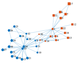
II-D2 Application to the southern woman network
The southern women network structure is analyzed and clustered them into groups in [2] based on interviews of 18 women. These 18 women attended 14 events and the connections among them are characterized by the number of co-attended events. Our partition algorithms assign individuals to two groups which is the same bipartition result except one node (node Pearl) as those in [2] and [40]. The partition result is as follows:
-
•
Cluster characterized by square-shaped nodes consists of Dorothy, Flora, Helen, Katherina, Myra, Nora, Olivia, Sylvia, Verne;
-
•
Cluster characterized by circle-shaped nodes consists of Brenda, Charlotte, Eleanor, Evelyn, Frances, Laura, Pearl, Ruth, Theresa.
as illustrated in Figure 2.
In contrast, the Fielder eigenvector of the original social network would partition nodes into two groups where one group only consists of Flora and Olivia, which is far from the real-world clustering result in [2]. This again indicates that the degree (centrality) weighted influence is important analyzing social network structures and opinion dynamics.

II-E Network partition into multiple groups
There are two ways to partition the graph into multiple clusters: 1) iterative bipartition and 2) -means. These two ways represent slightly different meanings of the partition.
II-E1 Iterative bipartition
Without initial opinion states and time constant, the partition of nodes on the network into different groups can be carried out as follows: First, we partition the graph into two subgraphs following our partition algorithm. Then we partition each of the subgraphs via our same partition algorithm. This procedure continues until the multiplicity of second smallest eigenvalue of the Laplacian for any graph or subgraph is more than . We then create a partition algorithm that can partition the graph into multiple groups. One feature of this partition method is that the number of clusters is automatically determined from the partition procedure and there is no need to specify the number of clusters beforehand.
II-E2 K-means
The vector produced by our algorithm approximately quantifies the disagreement level of individuals on the network. If the number of partitions is fixed and known beforehand, we can implement the standard -means [41] to cluster the approximate disagreement state values . We note that when has multiplicity more than 1, the initial opinion states is also needed. By clustering the disagreement states, we provide a partition of the nodes into different clusters, where different clusters represent nodes with different levels of disagreements. Furthermore, if both the time constant and the initial opinion states are known, then one can exactly characterize the evolution of the disagreement state and apply -means to identify time-varying clusters.
II-F Diversity of opinions
II-F1 Opinion diversity energy
Consider the following the energy function with
where . We note that here instead of is used. The opinion diversity energy at time is then given by
| (8) |
The opinion projected into the eigendirection associated with is given by
and the associated diversity energy is then given by
Remark 3
There may be other choices of the energy function with slightly different meanings, such as
□
II-F2 Inverse entropy diversity
If has multiplicity , we may use the following approximate estimate of the opinion diversity in (10), without considering the underlying time constant and initial condition . An entropy associated with can be defined via
| (9) |
where is the normalized Fiedler eigenvector (i.e., the normalized eigenvector with ). The diversity of opinions (or the size of disagreement) on the graph can then be characterized by
| (10) |
Since the property holds, the index takes into account the signs of implicitly. Roughly speaking, this index measures the diversity of the relative membership strengths of individuals to their own opinion groups.
Following the idea of Inverse Simpson index, another diversity measure can be given by
| (11) |
II-G The Markov chain interpretation
Following (2), each row of sums up to one and hence can be associated to the probability transition matrix of a Markov chain. Let represent the probability of individual support an idea or an opinion at time . Then the probability transition is characterized as follows: With probability (row) vector , the probability transition is compactly characterized by
| (12) |
This formulation follows the Degroot model [5] by specializing the influence matrix in [5] to be the degree-centrality-weighted matrix given by
Proposition 4 (Appendix -D)
If the underlying graph with the adjacency matrix is connected, then the Markov chain associated with as in (12) is irreducible and aperiodic if and only if is not an eigenvalue of . □
The diversity of the possible opinions at time can be estimated based on the inverse of the entropy of , that is, If with the adjacency matrix is undirected and connected and does not have eigenvalue , that is, the underlying Markov chain is irreducible and aperiodic, then for all and .
II-H General centrality-weighted opinion dynamics
Centralities on a network, which typically depend on the network structures, quantify the importance of nodes on the network. The degree centrality explored in Section II-A is a particular choice of centrality. Other examples of centralities included betweenness, eigen-centrality, page-rank centrality, Sharply values, etc. For different types of networks, different centralities may be suitable to characterize the influence on information and opinion propagation.
Similar to the previous model in Section II-A, the basic assumptions for general centrality-weighted opinion dynamics include the following:
-
(i)
Individual on a social network communicate and change their own opinions in the direction to conform with those of their neighbours;
-
(ii)
Each individual weights these influences from the neighbours based on their importance on the network quantified by the centrality vector .
The dynamic model for opinion state evolution over a network is then given by
where is the centrality of node on the network (based on an appropriate choice of centrality), is an appropriate time constant, and represents the connection from node to . The centrality should be chosen according to the underlying application problems, as different centralities may be suitable for different application problems. The Markov chain interpretation in (12) can also be generalized simply by replacing there by .
If for all , all the results in Propositions 1-4 hold for general centralities as well. The corresponding partition algorithm extends this this case naturally. Furthermore, one can verify that when the centrality is time-varying or state-dependent, all the results in Propositions 1-3 hold as long as for all .
III Conclusions
This paper proposed an opinion dynamics model based on network structures and nodal centralities. The model was used to partition graphs into clusters.
Future work should include exploring more real-world examples on different types of social networks, studying similar models for directed graphs, and providing a systematic procedure to identify suitable centralities based on data (i.e., the learning of the suitable centrality on social networks). Moreover, the centrality may also be generalized to depend on the opinion states or some equilibrium states.
IV Acknowledgement
The author would like to thank Prof. Peter Caines for the helpful conversations. [Proofs of Propositions 1-4]
-A Proof of Proposition 1
Proof
One can easily verify that , that is, is an eigenvalue of . Based on Gershgorin disk theorem [42], among all points on the imaginary axis only the origin can be the eigenvalue of , and all the eigenvalues except have strictly positive real parts. If any directed graph contains a rooted out-branching111A rooted out-branching on a directed graph is defined as the directed subgraph which is a directed tree, consists of all the nodes of the original graph, and contains a single root node (i.e., the node that has a directed path to all other nodes). , then the rank of the Laplacian matrix is (see for instance [39]). In the current case, since corresponds to an undirected and connected graph, we obtain that for all and furthermore we note that is the adjacency matrix of a strongly connected directed graph. Therefore corresponds to the adjacency matrix of a graph that contains a rooted out-branching. Hence as the associated Laplacian matrix has only one zero eigenvalue.■
-B Proof of Proposition 2
Proof
Let Since for any connected graph all the elements of and those of are non-zero, the inverse of exists and is given by Multiplying and on the left and right side of yields
| (13) | ||||
where . Since is symmetric, is also symmetric, and hence all the eigenvalues of are real. As is known that the similarity transformation preserves all eigenvalues, we obtain that all the eigenvalues of are real. Since , the eigenvalues for all . Therefore all the eigenvalues of are also real. ■
-C Proof of Proposition 3
Proof
Recall from (13) that
and is symmetric and obviously diagonalizable. Hence is diagonalizable. That is, there exist an invertible matrix and a diagonal matrix such that Hence . Therefore
that is, is diagonalizable. ■
-D Proof of Proposition 4
Proof
Since is connected, is strongly connected and hence the Markov chain associated with is irreducible. The aperiodicity is equivalent the fact that has only one eigenvalue that lies on the unit circle of the complex plane. Since all the eigenvalues of are real and is always an eigenvector of , the aperiodicity is equivalent to that is not an eigenvalue of . ■
References
- [1] W. W. Zachary, “An information flow model for conflict and fission in small groups,” Journal of Anthropological Research, vol. 33, no. 4, pp. 452–473, 1977.
- [2] A. Davis, B. B. Gardner, and M. R. Gardner, Deep South: A social anthropological study of caste and class, 1st ed. The University of Chicago Press, 1941.
- [3] A.-L. Barabási and R. Albert, “Emergence of scaling in random networks,” Science, vol. 286, no. 5439, pp. 509–512, 1999.
- [4] J. R. French Jr, “A formal theory of social power.” Psychological review, vol. 63, no. 3, p. 181, 1956.
- [5] M. H. DeGroot, “Reaching a consensus,” Journal of the American Statistical Association, vol. 69, no. 345, pp. 118–121, 1974.
- [6] N. E. Friedkin and E. C. Johnsen, “Social influence and opinions,” Journal of Mathematical Sociology, vol. 15, no. 3-4, pp. 193–206, 1990.
- [7] B. D. Anderson and M. Ye, “Recent advances in the modelling and analysis of opinion dynamics on influence networks,” International Journal of Automation and Computing, vol. 16, no. 2, pp. 129–149, 2019.
- [8] R. Hegselmann, U. Krause et al., “Opinion dynamics and bounded confidence models, analysis, and simulation,” Journal of artificial societies and social simulation, vol. 5, no. 3, 2002.
- [9] C. Altafini, “Consensus problems on networks with antagonistic interactions,” IEEE Transactions on Automatic Control, vol. 58, no. 4, pp. 935–946, 2012.
- [10] P. Jia, A. MirTabatabaei, N. E. Friedkin, and F. Bullo, “Opinion dynamics and the evolution of social power in influence networks,” SIAM review, vol. 57, no. 3, pp. 367–397, 2015.
- [11] Z. Xu, J. Liu, and T. Başar, “On a modified degroot-friedkin model of opinion dynamics,” in 2015 American Control Conference (ACC). IEEE, 2015, pp. 1047–1052.
- [12] A. V. Proskurnikov and R. Tempo, “A tutorial on modeling and analysis of dynamic social networks. part i,” Annual Reviews in Control, vol. 43, pp. 65–79, 2017.
- [13] R. Olfati-Saber and R. M. Murray, “Consensus protocols for networks of dynamic agents,” in Proceedings of the 2003 American Control Conference, 2003., vol. 2. IEEE, 2003, pp. 951–956.
- [14] A. Jadbabaie, J. Lin, and A. S. Morse, “Coordination of groups of mobile autonomous agents using nearest neighbor rules,” vol. 48, no. 6, pp. 988–1001, 2003.
- [15] Z. Lin, M. Broucke, and B. Francis, “Local control strategies for groups of mobile autonomous agents,” vol. 49, no. 4, pp. 622–629, 2004.
- [16] K. Sznajd-Weron and J. Sznajd, “Opinion evolution in closed community,” International Journal of Modern Physics C, vol. 11, no. 06, pp. 1157–1165, 2000.
- [17] G. Toscani et al., “Kinetic models of opinion formation,” Communications in mathematical sciences, vol. 4, no. 3, pp. 481–496, 2006.
- [18] G. Albi, L. Pareschi, and M. Zanella, “Opinion dynamics over complex networks: Kinetic modelling and numerical methods,” Kinetic & Related Models, vol. 10, no. 1, p. 1, 2017.
- [19] D. Acemoglu and A. Ozdaglar, “Opinion dynamics and learning in social networks,” Dynamic Games and Applications, vol. 1, no. 1, pp. 3–49, 2011.
- [20] A. Orléan, “Bayesian interactions and collective dynamics of opinion: Herd behavior and mimetic contagion,” Journal of Economic Behavior & Organization, vol. 28, no. 2, pp. 257–274, 1995.
- [21] M. A. Rahimian and A. Jadbabaie, “Bayesian learning without recall,” IEEE Transactions on Signal and Information Processing over Networks, vol. 3, no. 3, pp. 592–606, 2016.
- [22] R. Salhab, A. Ajorlou, and A. Jadbabaie, “Social learning with sparse belief samples,” in Proceedings of the 59th IEEE Conference on Decision and Control (CDC), 2020, pp. 1792–1797.
- [23] V. Kandiah and D. L. Shepelyansky, “Pagerank model of opinion formation on social networks,” Physica A: Statistical Mechanics and its Applications, vol. 391, no. 22, pp. 5779–5793, 2012.
- [24] S. Brin and L. Page, “The anatomy of a large-scale hypertextual web search engine,” Computer networks and ISDN systems, vol. 30, no. 1-7, pp. 107–117, 1998.
- [25] A. Singh, H. Cherifi et al., “Centrality-based opinion modeling on temporal networks,” IEEE Access, vol. 8, pp. 1945–1961, 2019.
- [26] M. Fiedler, “Algebraic connectivity of graphs,” Czechoslovak Mathematical Journal, vol. 23, no. 2, pp. 298–305, 1973.
- [27] A. Pothen, H. D. Simon, and K.-P. Liou, “Partitioning sparse matrices with eigenvectors of graphs,” SIAM journal on matrix analysis and applications, vol. 11, no. 3, pp. 430–452, 1990.
- [28] D. A. Spielman and S.-H. Teng, “Spectral partitioning works: Planar graphs and finite element meshes,” in Proceedings of 37th Conference on Foundations of Computer Science. IEEE, 1996, pp. 96–105.
- [29] M. E. Newman, “Modularity and community structure in networks,” Proceedings of the national academy of sciences, vol. 103, no. 23, pp. 8577–8582, 2006.
- [30] S. White and P. Smyth, “A spectral clustering approach to finding communities in graphs,” in Proceedings of the 2005 SIAM international conference on data mining. SIAM, 2005, pp. 274–285.
- [31] B. Peng, L. Zhang, and D. Zhang, “A survey of graph theoretical approaches to image segmentation,” Pattern recognition, vol. 46, no. 3, pp. 1020–1038, 2013.
- [32] M. E. Newman and M. Girvan, “Finding and evaluating community structure in networks,” Physical review E, vol. 69, no. 2, p. 026113, 2004.
- [33] M. Hoffman, D. Steinley, K. M. Gates, M. J. Prinstein, and M. J. Brusco, “Detecting clusters/communities in social networks,” Multivariate behavioral research, vol. 53, no. 1, pp. 57–73, 2018.
- [34] W. E. Donath and A. J. Hoffman, “Algorithms for partitioning of graphs and computer logic based on eigenvectors of connection matrices,” IBM Technical Disclosure Bulletin, vol. 15, no. 3, pp. 938–944, 1972.
- [35] ——, “Lower bounds for the partitioning of graphs,” IBM Journal of Research and Development, vol. 17, no. 5, pp. 420–425, 1973.
- [36] M. Fiedler, “Eigenvectors of acyclic matrices,” Czechoslovak Mathematical Journal, vol. 25, no. 4, pp. 607–618, 1975.
- [37] ——, “A property of eigenvectors of nonnegative symmetric matrices and its application to graph theory,” Czechoslovak Mathematical Journal, vol. 25, no. 4, pp. 619–633, 1975.
- [38] R. B. Cialdini and N. J. Goldstein, “Social influence: Compliance and conformity,” Annu. Rev. Psychol., vol. 55, pp. 591–621, 2004.
- [39] M. Mesbahi and M. Egerstedt, Graph Theoretic Methods in Multiagent Networks. Princeton University Press, 2010.
- [40] J. Liebig and A. Rao, “Identifying influential nodes in bipartite networks using the clustering coefficient,” in 2014 Tenth International Conference on Signal-Image Technology and Internet-Based Systems. IEEE, 2014, pp. 323–330.
- [41] D. Arthur and S. Vassilvitskii, “k-means++: The advantages of careful seeding,” Tech. Rep., 2006.
- [42] S. A. Gershgorin, “Uber die abgrenzung der eigenwerte einer matrix,” Bulletin del’Academie des Sciences de l’URSS. Classe des Sciences Mathematiques et na, vol. 6, pp. 749–754, 1931.