Central object segmentation by deep learning for fruits and other roundish objects
Abstract.
We present CROP (Central Roundish Object Painter), which identifies and paints the object at the center of an RGB image. Primarily CROP works for roundish fruits in various illumination conditions, but surprisingly, it could also deal with images of other organic or inorganic materials, or ones by optical and electron microscopes, although CROP was trained solely by 172 images of fruits. The method involves image segmentation by deep learning, and the architecture of the neural network is a deeper version of the original U-Net. This technique could provide us with a means of automatically collecting statistical data of fruit growth in farms. As an example, we describe our experiment of processing 510 time series photos automatically to collect the data on the size and the position of the target fruit. Our trained neural network CROP and the above automatic programs are available on GitHub (https://github.com/MotohisaFukuda/CROP), with user-friendly interface programs.
Key words and phrases:
Deep Learning, U-Net, Image Segmentation, Central Object, Fruits


1. Introduction
1.1. Computer vision and fruit cultivation
Techniques of computer vision have various applications in fruit production, for example making yield estimation by processing images of farms before the harvest. Such pre-harvest estimate is crucial for efficient resource allocations and these computer vision techniques certainly would constitute a part of smart agriculture [GAK+15].
To this end, initially, algorithms of human-made feature extraction engineering have been developed to locate fruits in camera images [DM04, NAB+11, MSD+16, PWSJ13, DLY17], and interestingly some used controlled illumination at night [NWA+14]. Also, non-destructive size and volume measurement of fruits is useful in production and distribution of fruits [MOCGRRA09]. This is in fact one of our motivations in this paper. Naturally computer vision techniques have been developed, for example using color analysis to conduct image segmentation [BSSR18]. Some used proper backgrounds for image segmentation [OKT10, MBMRMV+12], and even to develop a smart phone application [WKW+18].
Inevitably, machine learning techniques came in to play, for example for harvest estimation of tomatoes; image segmentation based on pixels and blobs and then X-means clustering were applied [YGYN14]. Even multi-spectral data was processed with conditional random field for image segmentation for various crops [HNT+13]. In addition, for robotic harvesting, examples include the uses of Viola-Jones object detection framework [PVTG16], and image segmentation with K-means clustering [WTZ+17]. For accurate size measurement, support vector machine performed image segmentation for apples with black backgrounds [ML13] for example.
1.2. Application of deep learning
Deep learning is one of machine learning techniques. There are more and more applications of deep learning not only in fruit production but also in agriculture as a whole [KPB18].
Human-made algorithms require humans to set features to be extracted from raw data. In this case, the number of such features must be limited if one wants to establish algorithms within a reasonable time frame. However, DNNs (Deep Neural Networks) extract important features automatically, which is one of key properties of deep learning. Of course, DNNs process data in a black box, but such data-driven methods could handle complex data, for example camera images in farms, which are affected heavily by time of day, weather conditions, seasons, and other illumination conditions such as shade and light reflection. Therefore, huge amount of features would be necessary in processing such images, and it would be simply too much for humans to find and list all important features in order to write algorithms by hand.
By contrast, things are completely different in processing data with DNNs, which consist of many layers. Roughly writing, as data flows in a DNN, each layer makes the data little more abstract, so that the DNN yields abstract understanding deep within itself. This way, humans do not have to pick important features by themselves. Interested readers can consult [GBC16] for more detailed theories of deep learning.
Recently one can find more and more applications of deep learning, for example counting apples [BU17b], apples and oranges [CSD+17], and tomatoes [RS17]. Also, in [WLS+20] deep learning was applied to image segmentation in order to obtain horizontal diameters of apples, by processing images taken on cloudy days or at dusk and pre-processed with Laplace transform. Moreover in [MPU17], light-weighted neural networks were developed for image segmentation for agricultural robotics.
Faster R-CNN [RHGS15] is one of famous DNNs for object detection, and yielded successful applications for example in detecting apples [BU17a], mangoes with spacial registration[LCL+19], and sweet papers by using multi-modal data (color and Near-infrared) [SGD+16]. Despite its popularity, Faster R-CNN has disadvantages; it gives rectangular bounding boxes for fruits in images but they do not give accurate size measurement. By contrast, human-made algorithms for object detection have aspects of image (semantic) segmentation, because they usually start with processing pixels to extract information such as colors and textures before finally detecting fruits. This way, object detection and image segmentation are often interwoven with each other in conventional techniques. In [SdSdSA20], however, instance segmentation via another DNN called Mask-RCNN [HHG+19] was used to overcome this disadvantage, together with space registration. One can find detailed explanations on application of Faster R-CNN and Mask-RCNN (and YOLOv3 [RF19]) to images of grapes in [SdSdSA20].
Our research put more weight on accurate measurement. Our neural network, which we call CROP (Central Roundish Object Painter), identifies and paints the fruit at the center of an image. It works for roundish fruits in various illumination conditions. This technique could provide us with a means of automatically collecting statistical data of fruit growth in farms, and perhaps might allow automated robots to make better decisions. We also developed programs to run CROP to automatically process time series photos by a fixed camera to collect the data on the size and the position of the target fruit; see Section 3.3. Our trained neural network CROP and the above automatic programs are available on GitHub (https://github.com/MotohisaFukuda/CROP), with user-friendly interface programs.
2. Results
2.1. Datasets
In this research project, we used several groups of images from the internet and farms in Kaminoyama, Yamagata, Japan, which are listed below with sample images.
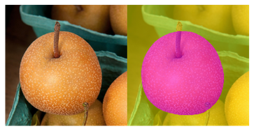
- Data_Fruits:
-
172 images of a variety of fruits downloaded from (https://pixabay.com).
![[Uncaptioned image]](https://cdn.awesomepapers.org/papers/3a4f5d31-4c4e-4332-b08f-6b2e3bcb031f/data0.png)
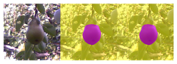
- Data_Pears1:
-
26 images of pears in the farm in 2018 with Brinno BCC100 (time-lapse mode).
![[Uncaptioned image]](https://cdn.awesomepapers.org/papers/3a4f5d31-4c4e-4332-b08f-6b2e3bcb031f/data1.png)
- Data_Pears2:
-
86 images of pears in the farm in 2019 with various cameras.
![[Uncaptioned image]](https://cdn.awesomepapers.org/papers/3a4f5d31-4c4e-4332-b08f-6b2e3bcb031f/data2.png)
Brinno BCC100 is a time-lapse camera used by one of the authors to keep track on growth of pears, which give blurred images to be processed.
These images were all annotated by labelme [Wad16] to train and evaluate CROP. In Section 4.3 quantitative analysis was conducted; we trained CROP with Data_Fruits being training data (80%) and validation data (20%), and afterwards fine-tuned it with Data_Pears2 being training data (80%) and validation data (20%). On the other hand, CROP in Section 2.2 was trained by all the images of Data_Fruits to make qualitative analysis.
2.2. Qualitative analysis
In this section, we show how CROP works by using sample images. We used all of Data_Fruits for training because we have a limited number of annotated images; we decided when to stop the training by processing random images on the internet. The sample images in this section do not belong to Data_Fruits, so that they can be thought of as test data, i.e. they are new to CROP. Predictions by CROP are represented by mask images pasted onto the original (cropped) images; red pixels for the central object and yellow for the rest.
In this section and the next, some of the original photos were provided by Hideki Murayama, or came from some institutions. In the latter case, they are credited in the captions, and the explanations of the acronyms of the institutions and the disclaimers are found in the section titled “About photos in this paper”.
First, the name of CROP does not come from the network architecture but from its function of identifying and painting the object at the center of an image. Examples in Figure 2(a) and Figure 2(b) indicate how CROP identifies individual grapes at the center of images. By contrast, CROP got confused in Figure 2(c) because the central grape was behind others. On the other hand, it even could handle wide-angle images like in Figure 2(d).


Let us go over some examples. Firstly, in Figure 3, one can see that CROP handled images of fruits of various shapes and colors.


Secondly, we classified common mistakes by CROP, and included representative examples in Figure 4. Here are our guesses why: in Figure 4(a), the object is not round enough, in Figure 4(b) the angle of two meeting boundaries is not acute enough, in Figure 4(c) there is a disruptive object, and in Figure 4(d) “ there is no boundary”. Thirdly, however, CROP can ignore those unimportant parts such as peduncle and calyx, like in Figure 5.


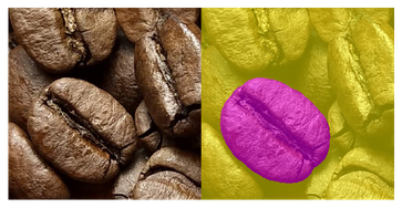
2.3. Acquiring general ability
Although CROP has been trained solely by 172 fruit images (no transfer learning or fine-tuning), it started to understand the meanings of boundaries of central roundish objects; some other foods than fruits in Figure 6, various materials some of which were through microscopes in Figure 7 , and photos in the space in Figure 8.


3. Applying CROP in real pear farms
One of the authors actually plans to apply CROP in pear production. We argue in this section why it is difficult to predict harvest time of pears and how we could adapt CROP to images in real usage conditions, so that one can collect time-series data of sizes of pears with fixed cameras in farms.
3.1. Pear production in Japan
“La France” is one of the most popular cultivars of European pear (Pyrus communis) in Japan, its yield is about 70% of European pears in Japan. La France pomes are usually harvested at the mature-green stage and then chilled for stimulation of ethylene biosynthesis prior to being ripened at the room temperature. If the harvest is delayed or too early, the fruit does not ripe properly, and the texture, taste and flavor will be poor. In commercial pear cultivation, harvest time of La France greatly influences both the amount and quality of the harvest. Therefore, it is important to measure the maturity of the fruit precisely to optimize the time to harvest, but criteria to estimate the fruit maturity are limited such as fruit firmness and blooming date. The fruit growth in terms of fruit size is described by an asymmetric sigmoid curve. The growth rate of the fruit on the tree is significantly affected by environmental factors and the physiologically active state. Precise time-lapse measurement of fruit growth should be useful for estimation of the fruit maturation status. In order to measure the fruit size change as it grows, the size of the same fruit must be measured repeatedly (daily) with a caliper.
Research on sizes of agricultural products, without computer vision, was previously conducted in predicting optimum harvest time of carrots [HS00], estimating yield of pears [Mit86] or anticipating cracking of bell peppers [NKG03]. Also devices for continuously measuring fruit size change have been developed, for example the kiwifruit volume meter (KVM) [GMA90], stainless frames with potentiometers to be put on fruits [MMZ+07], and flexible tapes around fruits to be read by infrared reflex sensors [Tha16]. However, one of the authors plans to estimate fruit size based on images, possibly by using CROP. We hope that our research will improve the accuracy of fruit size measurement and reduce the labor required in the data collection.
3.2. Getting fine-tuned for pears in farms
Since CROP was initially trained by clear images of various fruits of Data_Fruits, we used a technique called fine-tuning to re-train CROP by rather unclear images of pears of Data_Pears2, so that it can process similar images of Data_Pears1. One can consult Section 2.1 for these datasets, and Section 4.3 for quantitative analysis, where the effect of fine-tuning is investigated. In the rest of the section, however, let us make qualitative analysis of fine-tuning through examples.
In Figure 9, each triple consists of the original image, and images processed before and after the fine-tuning, placed from left to right. Some images were processed well even before the fine-tuning, like in Figure 9(a). There are some small improvements in Figures 9(b), 9(c), 9(d). Some showed dramatical improvement, like in Figure 9(e), and some on the contrary, like in Figure 9(f).
before after

before after


3.3. Application to time series photos
In this section, we show our way of using CROP in the local pear farms. All the implementations presented here are available on GitHub (https://github.com/MotohisaFukuda/CROP). We will focus on our method of collecting data and have no intention to draw any scientific conclusions, although we make some remarks based on the data. Indeed, eight photos were taken a day, at 8:00, 9:49, 11:49, 13:49, 15:49, 17:49, 19:49, 21:49, but the graphs and plots would look different if photos had been taken isochronously, for example once every three hours. In the following example, we processed 510 time series photos by a fixed camera to get the data on the size and the position of the chosen pear. All the process is automatic once we choose a target fruit in the first photo, and it took less than 14 minutes in this example. Note that these photos were taken in 2020 and are new to the CROP used in this section; see Section 2.1.
3.3.1. Applying CROP to time series photos
Now, we explain about the newly developed programs which process time series photos automatically. The key ideas are: CROP
-
(1)
is able to detect central objects.
-
(2)
may be applied in different scales and one can pick the median of the measurement outcomes.
-
(3)
can keep track of the 2D-wise center of mass of the target.
Let us elaborate the above three points one by one. First, once we specify an interested fruit by placing it around at the center of the photo frame (Figure 10(b)), then CROP can identify it, as in Figure 10(c). By applying this functionality repeatedly, CROP can keep track of the fruit across time-series photos taken by a fixed camera.
Secondly, the fact that some of incorrect predictions by CROP largely depend on angles enables us to take the median of several measurement outcomes of different angles. Our implementation of this idea can be seen in Figure 11, where inaccurate predictions in wider angles (Figure 11(a)) appear as outliers in the histogram (Figure 11(b)). Note that all the numbers of pixels were re-scaled back to in the scale of the original photo before taking the median. This is why the programs output a decimal as the number of pixels.
Thirdly, after choosing the best measurement in terms of median, one can also identify the center of mass in 2D photos (Figure 10(d)). We believe that this method is more reliable than using object detection algorithms. It is because errors in placing bounding boxes affect directly the positional data, but the center of mass is not so sensitive because pixel-wise mistakes will be averaged with other correct pixel-wise predictions.


3.3.2. Counting pixels and tracking the target
Now we discuss how we processed at once 510 () photos taken in Kaminoyama, Yamagata, Japan during 12 Aug 2020 13:49 –15 Oct 2020 8:00. Eight photos were taken a day, at 8:00, 9:49, 11:49, 13:49, 15:49, 17:49, 19:49, 21:49; the first three belong to the morning, the next two the afternoon, the last three the evening, in our terminology. No photos over night, unfortunately. The photos were given id’s from 2 to 511 chronologically. These photos were taken by SC-MB68 a trail camera from SINEI.
First, Figure 12 shows the graph of the variation of the size of the target fruit estimated by CROP. Unfortunately, there are terrible cases of miscounting; the worst four of which can be seen in Figure 13, where it was heavily misty.
Next, to have a closer look, we focus on the five days (08–12 Oct 2020; photo id’s are from 455 to 494) indicated by the highlight with cyan color in the graph. In Figure 14, apparently the fruit was larger in the evening, but we have to take account of optical effects by camera flash in the dark. Also, the eleven measurement outcomes tend to have high variance in the evening, which can be identified in the box plot in Figure 15, by longer boxes and whiskers, and more individual points, meaning that the data collected in the evening is less accurate. Nevertheless, we may be able to claim that it grew over night based only on the data during the daytime. Further, we focus on 12 Oct 2020, which corresponds to the yellow highlight in Figure 14. All the eight photos taken on the day and processed by CROP later are collected in Figure 16.


Finally, one can see how the target fruit moved around during the whole season in Figure 17(a); outlies are also included. Again, let’s focus on the above five days. In Figure 17(b), the fruit seems to have hung rather higher in the evening. With Figure 17(b), one can trace the movement chronologically, based on the predictions by CROP.


3.3.3. Remarks on technical matters
It took only 791.1025 seconds (less than 14 minutes) to process 510 photos with NVIDIA TITAN Xp a GPU. All the process was automatic after specifying the fruit as in Figure 10(b). During this process, for each photo, CROP made eleven measurements in different angles, stored the values as a csv file and all the mask images as thumbnails, chose the median and calculated the center of mass to save these data as a csv file and a PNG file. Without GPU it usually takes more than a minute to process just one photo, so use of a GPU is recommended for these new programs.
4. Methodology and quantitative analysis
In this section we make technical discussions. Our choices of neural networks and loss functions are described in Section 4.1 and Section 4.2, respectively. Then, in Section 4.3, quantitative analysis is made so that one can know how accurate predictions CROP could make for clear images, and what are affects of fine-tuning (see Section 3.2 as well). Also, Section 4.4 explains how one could get rather stable predictions with CROP through the averaging process, which was used in processing examples in this paper. Finally, we compare CROP with its original version of U-Net and argue that the improvement probably depends on the deeper structure of CROP.
4.1. Neural networks for image segmentation
Image segmentation can be seen as classification of image pixels. For example, if you want to cut out a fruit in an image, all you have to do is classify each pixel into one of two classes: fruit and background. The number of classes can be more than one, and in this case we want to classify each pixel into one of these classes. This kind of image process is called (image) semantic segmentation. In this sense, image semantic segmentation is much more difficult than object detection, where one classifies each image, and not each pixel. In the rest of this section we explain about our neural network and compare it with some other neural networks.
Strictly speaking, CROP is the name for our trained neural network for the specific purpose, however, we call our neural network CROP even before the training to avoid confusion. As in Figure 18(a), inputs of CROP are RGB -pixel images and outputs -pixel mask images. The downward red arrows represent convolutions with kernel and stride , which double the number of channels. Here, channel corresponds to another dimension than height and width, where the number of channels of RGB images is 3, and mask images 1. Similarly, the upward green arrows represent convolutions with kernel and stride , which however make the number of channels half. The red rectangles are concatenations of two convolutions with kernel and stride , which keep the number of channels unchanged. The green rectangles are again concatenations of convolutions, where the second convolutions are the same as the ones from the red rectangles, but the first ones are a bit different. Their inputs are direct sums (in the channel space) of the outputs of the layers below and the copies from the left, the latter of which are indicated by horizontal arrows. With these inputs then the first convolutions in the green rectangles make the number of channels half.
To make our explanation complete, we explain the first and last boxes. Pink and light green boxes represent again concatenations of convolutions with kernel and stride . Through these layers the number of channels change as and , respectively. Note that ReLU and batch normalization are applied adequately, which are not explicit in the figure.
The architecture of CROP is based on U-Net [RFB15]. U-Net was developed for medical image segmentation, and the architecture is depicted in Figure 18(b), which was taken from the website (https://lmb.informatik.uni-freiburg.de). After the emergence of U-Net, many related research projects were conducted, including V-Net for 3-dimensional medical images [MNA16], from which we took the loss function for our training.


U-Net (and V-net as well) belongs to the family of Fully Convolutional Networks (FCN), which is a subset of Convolutional Neural Networks (CNN). A CNN treats 2-dimensional data as it is, so that it gives better performance in image processing, and mathematically it is literally comparable to convolution operation. The idea of CNN is rather old [LHBB99] (some argue it comes from [Fuk80]). However, it proved useful in deep learning when AlexNet [KSH12] won ImageNet Large Scale Visual Recognition Challenge in 2012, which is an image classification contest. The key idea behind was that they combined the two ideas of CNN and Deep Neural Network (DNN). This new architecture, realized by computational power of GPUs, enabled the neural network to improve the error rate dramatically.
Naturally this architecture of (deep) FCN was then applied to the task of semantic segmentation in [LSD15], and with encoder-decoder structure in [NHH15] and [BKC17]. The encoder-decoder structure consists of two parts; encoding with convolutions or max pools and decoding with transposed convolutions or up samples. One can see this structure in the u-shaped part of U-Net. In Figure 18(b), an input RGB image of pixels becomes smaller by iterative application of max pools down to as small as , although the number of channels becomes , i.e. pixels are transformed into at the bottom, where U-Net processes the data “abstractly”. This down-sizing process corresponds to the . By contrast, through the decoder with up convolutions, U-Net yields an image of with channel size one, i.e. a mask image. Importantly, there are four skip connections, which are represented by horizontal gray arrows in Figure 18(b). They are supposed to transmit location information from the encoder to the decoder, and this architecture characterizes U-Net.
Now, CROP has a similar structure as in Figure 18(a). The biggest difference is that the decoder and encoder are much deeper than those of U-Net. CROP makes the size of an input image times smaller at the bottom, while U-Net nearly times smaller. Those numbers and correspond to the number of red down arrows in Figure 18(a) and Figure 18(b). We believe that this difference in depth enables CROP to have more global and abstract understanding of images; see Section 4.5 for quantitative experiments on this matter. Another difference is that we adopted convolutions with kernel and stride instead of max pools with kernel in the decoder, because convolutions learn but max pools do not. Note that “up convolution” in Figure 18(b) is same as “transposed convolution” in Figure 18(a).
Before concluding this section, we need to write about two more famous neural networks. The first one is an implementation of instance segmentation and is called Mask R-CNN [HHG+19]. Instance segmentation can distinguish neighboring objects of the same class, while semantic segmentation would mix them up because it would just classify the pixels of these objects to one class. Mask R-CNN was applied in [SdSdSA20], to detect grapes bunch-wise. However, since we choose a fruit and fix a camera in the first place (Section 3.1), we do not have to detect fruits and rather can focus on image segmentation. The second one, for semantic segmentation, is called DeepLabv3+ [CZP+18]. This neural network has atrous convolutions to capture contextual information, and works very well for general purposes. However, we do not need contextual information and would rather go for preciser segmentation ability of U-Net, which has been yielding many applications in medical image segmentation, where accuracy matters.
4.2. Loss functions for image segmentation
Loss functions tell neural networks how to improve themselves. In this sense, choice of loss function is very important in training neural networks. In this project, we picked soft dice loss [MNA16]:
| (1) |
where runs over all the pixels, pixels in our case. Here, are outputs of CROP and are the target (“the right answers”). As usual take values between and after going through the sigmoid function: , and exactly or . As for the latter, and correspond to pixels of the background and the object, respectively, and they are set based on the ground truth, i.e. annotated data. Note that the loss vanishes if for all ’s.
Among loss functions, pixel-wise cross entropy:
| (2) |
could seem to be a good choice if we consider image segmentation as classification of each pixel. In fact, the cross entropy loss is commonly used for image classification tasks. However, we did not use it because otherwise each pixel would carry the same share in (2). That is, in every batch, each mis-classified pixel makes the same amount of contribution to back-propagations (training process) regardless of the size of objects, and as a consequence, the neural network could learn to rather ignore small objects. By contrast, with soft dice loss as in (1), such imbalance would be compensated by regularization, which appears as the denominator. For similar reasons, we did not adopt loss ():
| (3) |
Note that the above soft dice loss is a variant of dice loss, This category of loss functions treat small and large objects relatively equally, and moreover if there are more than one classes they also modify imbalance among different classes. In [RFB15], they applied more penalty to boundaries to segment images of cells, but we did not follow their path to avoid complication.
Finally, IoU (Intersection over Union), or Jaccard index:
measures how two sets are close to each other. It takes the value between 0 and 1, corresponding to and , respectively. This is not a loss function but an evaluation criteria, but shares the same spirit.
4.3. Quantitative analysis of training process
In this subsection, we give data-scientific evaluation of the training process of CROP, by using soft dice loss and IoU. All the evaluations were made with data augmentation unless otherwise stated.
4.3.1. Training CROP
For quantitative analysis we divided Data_Fruits into the training dataset (80%: 137) and the validation dataset (20%: 35). Initial parameters of CROP were set randomly (we did not use pre-trained models), and were then “optimized” by Adam with learning rate and with batch size 14. The result can be seen in Figure 19, where the best IoU for the validation data was 0.985, achieved at the epoch 8,700. To understand this value, suppose that we have a ground truth and a prediction of 100 pixels each, and that 99 pixels are correctly predicted. Then, the IoU would be:
This optimal CROP was saved to the network dictionary named “net_dic_0601_08700’ on GitHub, and was applied to examples in Section 3.2 to give predictions before the fine-tuning.
Note that CROP in Section 2.2 and Section 2.3 were trained on all the images of Data_Fruits and the training was stopped at epoch 5,000, which seemed optimal through random samples on the internet. The network dictionary is named “net_dic_0314_05000” on GitHub.


4.3.2. Fine-tuning CROP
For fine-tuning, we divided Data_Pears2 into the training dataset (80%: 68) and the validation dataset (20%: 18). Then, we retrained the optimal CROP from Section 4.3.1, through optimization by Adam with learning rate 0.0001 and with batch size 14. One can see the process in Figure 20. The best IoU for the validation data was 0.982, achieved at the epoch 5,200. This optimal CROP was applied to examples in Section 3.2. This network dictionary is named “net_dic_ft_0601_05200” and placed on GitHub. We also fine-tuned “net_dic_0314_05000” for 5000 epochs to get the dictionary “net_dic_ft_0328_1_5000”, which was used in Section 3.3 and is on GitHub.
Although, the improvement seems small from the graph in Figure 20, the IoU for Data_Pears1 improved a lot, which can be seen on Table 1, where data augmentation was not applied because a good portion of the images in Data_Pears1 are already blur.


| before | after | |
| IoU | 0.605 | 0.938 |
4.4. In using CROP
To make the predictions stable, we feed CROP eight different images made by applying actions of the dihedral group to the original input image. They are eight different combinations of flips and rotations which keep a square unchanged in the two-dimensional space. The final decision was made by averaging the corresponding eight predictions by CROP. This is how we applied CROP to the examples in this paper, and it is implemented on GitHub, but the functionality can be switched off for quicker and possibly less accurate predictions.
4.5. Discussions on depth of neural networks
In this section, we report on experiments on the shallow version of CROP, which is comparable to the original U-Net. Provisionally we call it CROP-Shallow (see Figure 21). To this end, we trained CROP-Shallow and CROP in the same condition: loss function, optimization method, learning rate, but random were partitions of training and validation sets, initialization of these neural networks, choice of batches and application of data augmentation. Also, the batch size was fixed to 6 for CROP-Shallow, which consumes a lot of GPU memory probably because of the way how the channel size (or feature map size) changes. However, the number of parameters itself is much smaller than that of CROP; 40,103,873 for CROP-Shallow and 160,829,681 for CROP.
Despite these potential problems, however, we still believe that we captured significant difference between the two architectures. See Figure 22, which shows over-fitting. The difference can be read also from Table 2 of IoUs for the validation datasets.


| CROP | CROP-Shallow | |
| best IoU | 0.985 | 0.899 |


5. Discussions on future directions
As described above CROP was trained solely by 172 fruit images. With more training data, it would increase accuracy and generality. For accuracy, CROP comes with a disadvantage that it is heavy. It would need to slim down if it is to be used for harvesting robots, for example, where spontaneous data processing is required.
In this project, we witnessed CROP had gained general ability to find the boundaries of various types of objects at the center of images. However, it is different from salient object detection [LHK+14], as CROP identifies a small central object like the one in Figure 2(d). Perhaps, techniques developed in this paper could be applied to portrait segmentation [STG+16, SHJ+16, DWL+19], or image segmentation for central objects in images, which we call central image segmentation.
About photos in this paper
Example photos in this papers were provided by Motohisa Fukuda, Hideki Murayama and Takashi Okuno as well as the following institutions, which are indicated by the acronyms. Original photos were cropped and processed by CROP.
-
•
CDC: Centers for Disease Control and Prevention (USA). Use of Centers for Disease Control and Prevention (CDC) photos is not meant to serve as an official endorsement of any particular product or company, by the CDC, HHS, or the United States government.
-
•
NASA: National Aeronautics and Space Administration (USA). Use of photos of National Aeronautics and Space Administration (NASA) does not state or imply the endorsement by NASA or by any NASA employee of a commercial product, service, or activity.
-
•
USDA ARS: United States Department of Agriculture, Agricultural Research Service (USA). Use of photos of Agricultural Research Service (ARS) of United States Department of Agriculture (USDA) is not meant to infer or imply ARS endorsement of any product, company, or position.
Acknowledgement
M.F. gratefully acknowledges the support of NVIDIA Corporation with the donation of the TITAN Xp GPU. M.F. was financially supported by Leibniz Universität Hannover to present the result and have fruitful discussions in Hannover. M.F. thanks his colleague Richard Jordan for having a discussion with him to name our trained neural network and for suggesting better expressions in the title and abstract. M.F. and T.O. were financially supported by Yamagata University (YU-COE program). T.O. thanks Kazumi Sato and Yota Ozeki, who let him take images of pears in the farms, and Yota Sato for annotating Data_Pears2. The authors also thank Kazunari Adachi of the engineering department for giving us valuable legal advice concerinig this research project, and Hideki Murayama of the agricultural department for providing us with photos of fruits.
References
- [BKC17] Vijay Badrinarayanan, Alex Kendall, and Roberto Cipolla. Segnet: A deep convolutional encoder-decoder architecture for image segmentation. IEEE transactions on pattern analysis and machine intelligence, 39(12):2481–2495, 2017.
- [BSSR18] Santi Kumari Behera, Shrabani Sangita, Prabira Kumar Sethy, and Amiya Kumar Rath. Image processing based detection & size estimation of fruit on mango tree canopies. International Journal of Applied Engineering Research, 13(4), 2018.
- [BU17a] Suchet Bargoti and James Underwood. Deep fruit detection in orchards. In 2017 IEEE International Conference on Robotics and Automation (ICRA), pages 3626–3633. IEEE, 2017.
- [BU17b] Suchet Bargoti and James P Underwood. Image segmentation for fruit detection and yield estimation in apple orchards. Journal of Field Robotics, 34(6):1039–1060, 2017.
- [CSD+17] Steven W Chen, Shreyas S Shivakumar, Sandeep Dcunha, Jnaneshwar Das, Edidiong Okon, Chao Qu, Camillo J Taylor, and Vijay Kumar. Counting apples and oranges with deep learning: A data-driven approach. IEEE Robotics and Automation Letters, 2(2):781–788, 2017.
- [CZP+18] Liang-Chieh Chen, Yukun Zhu, George Papandreou, Florian Schroff, and Hartwig Adam. Encoder-decoder with atrous separable convolution for semantic image segmentation. In Proceedings of the European conference on computer vision (ECCV), pages 801–818, 2018.
- [DLY17] Ulzii-Orshikh Dorj, Malrey Lee, and Sang-seok Yun. An yield estimation in citrus orchards via fruit detection and counting using image processing. Computers and Electronics in Agriculture, 140:103–112, 2017.
- [DM04] Gregory M Dunn and Stephen R Martin. Yield prediction from digital image analysis: A technique with potential for vineyard assessments prior to harvest. Australian Journal of Grape and Wine Research, 10(3):196–198, 2004.
- [DWL+19] Xianzhi Du, Xiaolong Wang, Dawei Li, Jingwen Zhu, Serafettin Tasci, Cameron Upright, Stephen Walsh, and Larry Davis. Boundary-sensitive network for portrait segmentation. In 2019 14th IEEE International Conference on Automatic Face & Gesture Recognition (FG 2019), pages 1–8. IEEE, 2019.
- [Fuk80] Kunihiko Fukushima. Neocognitron: A self-organizing neural network model for a mechanism of pattern recognition unaffected by shift in position. Biological cybernetics, 36(4):193–202, 1980.
- [GAK+15] A Gongal, Suraj Amatya, Manoj Karkee, Q Zhang, and Karen Lewis. Sensors and systems for fruit detection and localization: A review. Computers and Electronics in Agriculture, 116:8–19, 2015.
- [GBC16] Ian Goodfellow, Yoshua Bengio, and Aaron Courville. Deep learning. MIT press, 2016.
- [GMA90] AE Green, KJ McAneney, and MS Astill. An instrument for measuring kiwifruit size. New Zealand journal of crop and horticultural science, 18(2-3):115–120, 1990.
- [HHG+19] Zhaojin Huang, Lichao Huang, Yongchao Gong, Chang Huang, and Xinggang Wang. Mask scoring r-cnn. In Proceedings of the IEEE Conference on Computer Vision and Pattern Recognition, pages 6409–6418, 2019.
- [HNT+13] Calvin Hung, Juan Nieto, Zachary Taylor, James Underwood, and Salah Sukkarieh. Orchard fruit segmentation using multi-spectral feature learning. In 2013 IEEE/RSJ International Conference on Intelligent Robots and Systems, pages 5314–5320. IEEE, 2013.
- [HS00] F Hahn and S Sanchez. Carrot volume evaluation using imaging algorithms. Journal of agricultural engineering research, 75(3):243–249, 2000.
- [KPB18] Andreas Kamilaris and Francesc X Prenafeta-Boldú. Deep learning in agriculture: A survey. Computers and electronics in agriculture, 147:70–90, 2018.
- [KSH12] Alex Krizhevsky, Ilya Sutskever, and Geoffrey E Hinton. Imagenet classification with deep convolutional neural networks. In Advances in neural information processing systems, pages 1097–1105, 2012.
- [LCL+19] Xu Liu, Steven W Chen, Chenhao Liu, Shreyas S Shivakumar, Jnaneshwar Das, Camillo J Taylor, James Underwood, and Vijay Kumar. Monocular camera based fruit counting and mapping with semantic data association. IEEE Robotics and Automation Letters, 4(3):2296–2303, 2019.
- [LHBB99] Yann LeCun, Patrick Haffner, Léon Bottou, and Yoshua Bengio. Object recognition with gradient-based learning. In Shape, contour and grouping in computer vision, pages 319–345. Springer, 1999.
- [LHK+14] Yin Li, Xiaodi Hou, Christof Koch, James M Rehg, and Alan L Yuille. The secrets of salient object segmentation. In Proceedings of the IEEE Conference on Computer Vision and Pattern Recognition, pages 280–287, 2014.
- [LSD15] Jonathan Long, Evan Shelhamer, and Trevor Darrell. Fully convolutional networks for semantic segmentation. In Proceedings of the IEEE conference on computer vision and pattern recognition, pages 3431–3440, 2015.
- [MBMRMV+12] Eduardo A Murillo-Bracamontes, Miguel E Martinez-Rosas, Manuel M Miranda-Velasco, Horacio L Martinez-Reyes, Jesus R Martinez-Sandoval, and Humberto Cervantes-de Avila. Implementation of hough transform for fruit image segmentation. Procedia Engineering, 35:230–239, 2012.
- [Mit86] PD Mitchell. Pear fruit growth and the use of diameter to estimate fruit volume and weight. HortScience, 21(4):1003–1005, 1986.
- [ML13] Akira Mizushima and Renfu Lu. An image segmentation method for apple sorting and grading using support vector machine and otsu’s method. Computers and electronics in agriculture, 94:29–37, 2013.
- [MMZ+07] Brunella Morandi, Luigi Manfrini, Marco Zibordi, Massimo Noferini, Giovanni Fiori, and Luca Corelli Grappadelli. A low-cost device for accurate and continuous measurements of fruit diameter. HortScience, 42(6):1380–1382, 2007.
- [MNA16] Fausto Milletari, Nassir Navab, and Seyed-Ahmad Ahmadi. V-net: Fully convolutional neural networks for volumetric medical image segmentation. In 2016 Fourth International Conference on 3D Vision (3DV), pages 565–571. IEEE, 2016.
- [MOCGRRA09] GP Moreda, J Ortiz-Cañavate, Francisco Javier García-Ramos, and Margarita Ruiz-Altisent. Non-destructive technologies for fruit and vegetable size determination–a review. Journal of Food Engineering, 92(2):119–136, 2009.
- [MPU17] Chris McCool, Tristan Perez, and Ben Upcroft. Mixtures of lightweight deep convolutional neural networks: Applied to agricultural robotics. IEEE Robotics and Automation Letters, 2(3):1344–1351, 2017.
- [MSD+16] Christopher McCool, Inkyu Sa, Feras Dayoub, Christopher Lehnert, Tristan Perez, and Ben Upcroft. Visual detection of occluded crop: For automated harvesting. In 2016 IEEE International Conference on Robotics and Automation (ICRA), pages 2506–2512. IEEE, 2016.
- [NAB+11] Stephen Nuske, Supreeth Achar, Terry Bates, Srinivasa Narasimhan, and Sanjiv Singh. Yield estimation in vineyards by visual grape detection. In 2011 IEEE/RSJ International Conference on Intelligent Robots and Systems, pages 2352–2358. IEEE, 2011.
- [NHH15] Hyeonwoo Noh, Seunghoon Hong, and Bohyung Han. Learning deconvolution network for semantic segmentation. In Proceedings of the IEEE international conference on computer vision, pages 1520–1528, 2015.
- [NKG03] Mathieu Ngouajio, William Kirk, and Ronald Goldy. A simple model for rapid and nondestructive estimation of bell pepper fruit volume. HortScience, 38(4):509–511, 2003.
- [NWA+14] Stephen Nuske, Kyle Wilshusen, Supreeth Achar, Luke Yoder, Srinivasa Narasimhan, and Sanjiv Singh. Automated visual yield estimation in vineyards. Journal of Field Robotics, 31(5):837–860, 2014.
- [OKT10] M Omid, M Khojastehnazhand, and A Tabatabaeefar. Estimating volume and mass of citrus fruits by image processing technique. Journal of food Engineering, 100(2):315–321, 2010.
- [PVTG16] Steven Puttemans, Yasmin Vanbrabant, Laurent Tits, and Toon Goedemé. Automated visual fruit detection for harvest estimation and robotic harvesting. In 2016 Sixth International Conference on Image Processing Theory, Tools and Applications (IPTA), pages 1–6. IEEE, 2016.
- [PWSJ13] Alison B Payne, Kerry B Walsh, PP Subedi, and Dennis Jarvis. Estimation of mango crop yield using image analysis–segmentation method. Computers and electronics in agriculture, 91:57–64, 2013.
- [RF19] Joseph Redmon and Ali Farhadi. Yolov3: An incremental improvement. arxiv 2018. arXiv preprint arXiv:1804.02767, 2019.
- [RFB15] Olaf Ronneberger, Philipp Fischer, and Thomas Brox. U-net: Convolutional networks for biomedical image segmentation. In International Conference on Medical image computing and computer-assisted intervention, pages 234–241. Springer, 2015.
- [RHGS15] Shaoqing Ren, Kaiming He, Ross Girshick, and Jian Sun. Faster r-cnn: Towards real-time object detection with region proposal networks. In Advances in neural information processing systems, pages 91–99, 2015.
- [RS17] Maryam Rahnemoonfar and Clay Sheppard. Deep count: fruit counting based on deep simulated learning. Sensors, 17(4):905, 2017.
- [SdSdSA20] Thiago T Santos, Leonardo L de Souza, Andreza A dos Santos, and Sandra Avila. Grape detection, segmentation, and tracking using deep neural networks and three-dimensional association. Computers and Electronics in Agriculture, 170:105247, 2020.
- [SGD+16] Inkyu Sa, Zongyuan Ge, Feras Dayoub, Ben Upcroft, Tristan Perez, and Chris McCool. Deepfruits: A fruit detection system using deep neural networks. Sensors, 16(8):1222, 2016.
- [SHJ+16] Xiaoyong Shen, Aaron Hertzmann, Jiaya Jia, Sylvain Paris, Brian Price, Eli Shechtman, and Ian Sachs. Automatic portrait segmentation for image stylization. In Computer Graphics Forum, volume 35, pages 93–102. Wiley Online Library, 2016.
- [STG+16] Xiaoyong Shen, Xin Tao, Hongyun Gao, Chao Zhou, and Jiaya Jia. Deep automatic portrait matting. In European conference on computer vision, pages 92–107. Springer, 2016.
- [Tha16] Martin Thalheimer. A new optoelectronic sensor for monitoring fruit or stem radial growth. Computers and Electronics in Agriculture, 123:149–153, 2016.
- [Wad16] Kentaro Wada. labelme: Image Polygonal Annotation with Python. https://github.com/wkentaro/labelme, 2016.
- [WKW+18] Zhenglin Wang, Anand Koirala, Kerry Walsh, Nicholas Anderson, and Brijesh Verma. In field fruit sizing using a smart phone application. Sensors, 18(10):3331, 2018.
- [WLS+20] Dandan Wang, Changying Li, Huaibo Song, Hongting Xiong, Chang Liu, and Dongjian He. Deep learning approach for apple edge detection to remotely monitor apple growth in orchards. IEEE Access, 8:26911–26925, 2020.
- [WTZ+17] Chenglin Wang, Yunchao Tang, Xiangjun Zou, Weiming SiTu, and Wenxian Feng. A robust fruit image segmentation algorithm against varying illumination for vision system of fruit harvesting robot. Optik, 131:626–631, 2017.
- [YGYN14] Kyosuke Yamamoto, Wei Guo, Yosuke Yoshioka, and Seishi Ninomiya. On plant detection of intact tomato fruits using image analysis and machine learning methods. Sensors, 14(7):12191–12206, 2014.