This paper was converted on www.awesomepapers.org from LaTeX by an anonymous user.
Want to know more? Visit the Converter page.

Central limit theorem for linear spectral statistics of block-Wigner-type matrices

Zhenggang Wanglabel=e1][email protected] [    Jianfeng Yaolabel=e2][email protected] [ Department of Statistics and Actuarial Science, The University of Hong Kong, Department of Statistics and Actuarial Science, The University of Hong Kong,
Abstract

Motivated by the stochastic block model, we investigate a class of Wigner-type matrices with certain block structures, and establish a CLT for the corresponding linear spectral statistics via the large-deviation bounds from local law and the cumulant expansion formula. We apply the results to the stochastic block model. Specifically, a class of renormalized adjacency matrices will be block-Wigner-type matrices. Further, we show that for certain estimator of such renormalized adjacency matrices, which will be no longer Wigner-type but share long-range non-decaying weak correlations among the entries, the linear spectral statistics of such estimators will still share the same limiting behavior as those of the block-Wigner-type matrices, thus enabling hypothesis testing about stochastic block model.

60B20,
60F05,
15B52,
Wigner-type matrices,
stochastic block model,
linear spectral statistics,
keywords:
[class=MSC2020]
keywords:
\startlocaldefs\endlocaldefs

, and

1 Introduction

The investigation into the limiting properties of large random matrices has been popular for over two decades. Many techniques [8][6][13][18] are developed to solve problems in this area. There are plenty of objects of interest, namely the empirical spectral distribution (ESD), the limiting spectral distribution(LSD), the largest eigenvalue, the linear spectral statistics (LSS), the eigenvector statistics, etc. Particularly, the linear spectral statistics have attracted lots of attention ever since the 90s [28]. Various methods are explored to study the behavior of the LSS, such as moment method [5], martingale difference method [7][9], cumulant expansion method [22]. Also there is progress from the stochastic calculus [17][20] and free probability [27]. Further, [14][15] generalize the Stein method and use second order Poincaré inequalities to prove a CLT for the LSS. Specifically, in recent years, a more in-depth understanding of the behavior of the LSS of Wigner and Wigner-type matrices has been achieved by researchers from various perspectives. [26] introduces an interpolation method for more general Wigner matrices than the ones that share the same cumulants with GOE/GUE. [12] extends the CLT to certain heavy-tailed random matrices. More recently, [21] studies the mesoscopic eigenvalue statistics of the Wigner matrices via the Green function and the local law, [16] yields a thorough analysis of fluctuations of regular functions of Wigner matrices and [11] establishes a near-optimal convergence rate for the CLT of LSS of Wigner matrices.

In the meantime, motivations are drawn from social networks and other associated random graph models, which brings the researchers’ attention to more involved matrix models. One of the most classic models in this field is the stochastic block model (SBM). In contrast to the Erdős-Renyi model in which all nodes are exchangeable, the SBM introduces inhomogeneity by dividing the nodes into different communities. In the SBM with nodes VV and edges EE, all edges are undirected, and different edges are independent, in the meantime, the probability that two nodes vi,vjVv_{i},v_{j}\in V connect with each other is only determined by which communities viv_{i} and vjv_{j} belong to. In other words, the adjacency matrix of the SBM can be viewed as a random 0-1 matrix whose entries have block-wise constant expectations. Thus, the centered adjacency matrices of the SBMs are Wigner-type matrices with inhomogeneous variance profiles.

One of the most important questions in the SBM is community detection, which is to recover the community structure underneath via one single observation of the adjacency matrix. Further, an induced problem is to determine the number of communities. For most community detection algorithms, the number of communities needs to be given a priori as a hyperparameter. This motivates hypothesis testing for this parameter via the distributional information of certain test statistics of the model. [25] proposes a sequential test for the renormalized adjacency matrix (Aijpijnpij(1pij))ij\left(\frac{A_{ij}-{p}_{ij}}{\sqrt{np_{ij}(1-p_{ij})}}\right)_{ij} and (Aijp^ijnp^ij(1p^ij))ij\left(\frac{A_{ij}-\hat{p}_{ij}}{\sqrt{n\hat{p}_{ij}(1-\hat{p}_{ij})}}\right)_{ij} based on the Tracy-Widom fluctuation of the largest eigenvalue. In the same spirit, more recently in [10], Banerjee and Ma propose a hypothesis testing for the community structure via the LSS of the renormalized adjacency matrix (Aijp^ijnp^ij(1p^ij))ij\left(\frac{A_{ij}-\hat{p}_{ij}}{\sqrt{n\hat{p}_{ij}(1-\hat{p}_{ij})}}\right)_{ij} with the method of moments approach [5] in the cases where the SBM has only one community or two asymptotically equal-sized communities. Towards another end, [1] proves a CLT for the LSS of general Wigner-type matrices via the second order Poincaré inequality without providing the explicit formulas for the asymptotic mean and covariance function.

In this paper, We establish CLTs for the class of block-Wigner-type matrices which is motivated by the renormalization (Aijpijn)\left(\frac{A_{ij}-p_{ij}}{\sqrt{n}}\right) as well as a correlated matrix model induced from the renormalization (Aijp^ijn)\left(\frac{A_{ij}-\hat{p}_{ij}}{\sqrt{n}}\right). We derive the explicit formulas for the asymptotic mean functions and covariance functions with the help of precise large deviation estimates of the Green function by [4] and the application of cumulant expansion formula [22][19].

Our contributions.

We strengthen the existing results in the following ways:

  1. 1.

    Our block-Wigner-type matrices may have not only inhomogeneous fourth moments but also inhomogeneous second moments. This greatly extends the potential range of application of the theorem. We show that the approximately low-rank structure of the entries would reproduce itself in terms of repetitive patterns in the system of equations for key moments of Tr(G(z))Tr(G(z)) and other related higher-order structures.

  2. 2.

    Further, we establish a CLT for the LSS of the data-driven variation of the above matrices, which is no longer Wigner-type and shares long-range weak correlations among the entries. This yields a direct application in the SBM.

Organization

We first introduce a few prerequisites about our main tools and ingredients in Section 2. Then we introduce the block-Wigner-type matrices and establish the CLT for LSS of such matrices in Section 3.1. In Section 3.2, we consider the application to the SBM and establish a new CLT for LSS of a data-driven variation of the block-Wigner-type matrices. In Section 4, the outlines of the proofs of the main results are shown. In Section 5, we apply the above 2 CLTs to the synthetic data of the SBM to show the efficiency of the theorems. Details of proofs are shown in Section A and B.

2 Preliminary

2.1 Notation

For simplicity of presentation, we will use M¯\underline{M} for normalized trace 1NTr(M)\frac{1}{N}Tr(M) of a n×nn\times n square matrix MM, R\langle R\rangle to denote centered version R𝔼RR-\mathbb{E}R of a random variable RR, and [K]={1,2,,K}[K]=\{1,2,\cdots,K\} to represent the set of positive integers from 1 to KK. Further, we introduce two operations related to diagonal terms: for a column vector 𝐯=[v1,,vn]\mathbf{v}=[v_{1},\cdots,v_{n}]^{\top}, Diag[𝐯]Diag[\mathbf{v}] denotes the diagonal matrix whose diagonal elements are the entries of 𝐯\mathbf{v}, and for a n×nn\times n matrix MM, diag(M)diag(M) denotes the column vector whose entries are the diagonal element of MM. In particular, diagøDiag=Iddiag\o\circ Diag=Id.

2.2 Large deviation bounds from local law for Wigner-type matrices

This section gives a quick review of the large deviation bounds from the local law for general Wigner-type matrices by Ajanki et al. [3][4], which will serve as one of the main ingredients for proving our central limit theorem.

The main object of interest is the resolvent G(z)=(Hz)1G(z)=(H-z)^{-1}, where HH is the so-called Wigner-type matrix such that HH is real symmetric and the entries HijH_{ij} are independent for iji\leq j and centered 𝔼Hij=0,i,j[n]\mathbb{E}H_{ij}=0,\ \forall i,j\in[n].

Let S=(sij)i,j=1n=(𝔼|Hij|2)i,j=1nS=(s_{ij})_{i,j=1}^{n}=(\mathbb{E}|H_{ij}|^{2})_{i,j=1}^{n}, then the system of the quadratic vector equations (QVE) is

1mi(z)=z+j=1nsijmj(z), for all i[n],z+.-\frac{1}{m_{i}(z)}=z+\sum_{j=1}^{n}s_{ij}m_{j}(z),\quad\text{ for all }\quad i\in[n],\quad z\in\mathbb{C}_{+}. (1)

There exists a unique solution 𝐦=(m1,,mn):++n\mathbf{m}=(m_{1},\ldots,m_{n}):\mathbb{C}_{+}\rightarrow\mathbb{C}_{+}^{n} of the above system on the complex upper half-plane. We refer the readers to [3] for properties of the QVE system. It is proved by Ajanki et al. [4] that under certain regularity conditions, the solution 𝐦=(m1,,mn)\mathbf{m}=(m_{1},\ldots,m_{n}) of the above system of equations may serve as a good approximation for the diagonal terms (G11,,Gnn)(G_{11},\ldots,G_{nn}) of the resolvent.

Definition 2.1 (Stochastic domination).

Suppose N0:(0,)2N_{0}:(0,\infty)^{2}\rightarrow\mathbb{N} is a given function, depending only on certain model parameters. For two sequences, φ=(φ(N))N\varphi=\left(\varphi^{(N)}\right)_{N} and ψ=(ψ(N))N,\psi=\left({\psi}^{(N)}\right)_{N}, of non-negative random variables we say that φ\varphi is stochastically dominated by ψ\psi if for all ε>0\varepsilon>0 and D>0,D>0,

(φ(N)>Nεψ(N))ND,NN0(ε,D).\mathbb{P}\left(\varphi^{(N)}>N^{\varepsilon}\psi^{(N)}\right)\leq N^{-D},\quad N\geq N_{0}(\varepsilon,D).

In this case we write φψ\varphi\prec\psi or φ=O(ψ)\varphi=O_{\prec}(\psi).

Lemma 2.2 (Theorem 1.7 of [4], reformulated to a macroscopic version).

Let HH be a Wigner-type matrix and 𝐦\mathbf{m} be defined in (1). Suppose that the following assumptions hold:

  1. A

    For all nn the matrix S\mathrm{S} is flat, i.e.,

    sijCn,C>0,i,j[n];s_{ij}\leq\frac{C}{n},\quad C>0,\quad i,j\in[n];
  2. B

    For all nn the matrix SS is uniformly primitive, i.e.;

    (SL)ijpn,p>0,i,j[n],\left(S^{L}\right)_{ij}\geq\frac{p}{n},\ p>0,\quad i,j\in[n],
  3. C

    For all nn the entries HijH_{ij} of the random matrix HH have bounded moments

    𝔼|Hij|kμksijk/2,k,i,j[n].\mathbb{E}\left|H_{ij}\right|^{k}\leq\mu_{k}s_{ij}^{k/2},\quad k\in\mathbb{N},i,j\in[n].

are satisfied. Then uniformly for all z=τ+iη+z=\tau+i\eta\in\mathbb{C}_{+} with constant order imaginary part η\eta or real part τ\tau that is bounded away from the edge of the spectrum of HH, the resolvents of the random matrices H=H(n)H=H^{(n)} satisfy

maxi,j|Gij(z)mi(z)δij|=O(1n).\max_{i,j}|G_{ij}(z)-m_{i}(z)\delta_{ij}|=O_{\prec}(\frac{1}{\sqrt{n}}). (2)

Furthermore, for any sequence of deterministic vectors 𝐰=𝐰(n)=[w1,,wn]n\boldsymbol{w}=\boldsymbol{w}^{(n)}=[w_{1},\cdots,w_{n}]\in\mathbb{C}^{n} with maxi|wi|1\max_{i}|w_{i}|\leq 1, the averaged resolvent diagonal has an improved convergence rate.

|1ni=1nw¯i(Gii(z)mi(z))|=O(1n).|\frac{1}{n}\sum_{i=1}^{n}\bar{w}_{i}(G_{ii}(z)-m_{i}(z))|=O_{\prec}(\frac{1}{n}). (3)

A direct application of Lemma 2.2 together with the trivial bound |Gij(z)|1|z||G_{ij}(z)|\leq\frac{1}{|\Im z|} leads to the following corollary, whose proof is omitted.

Corollary 2.3.

ε>0,K0\forall\varepsilon>0,K_{0}\in\mathbb{N}, there exists a Nε,K0N_{\varepsilon,K_{0}} s.t. when nNε,K0n\geq N_{\varepsilon,K_{0}},

𝔼|Gij(z)δijmi(z)|knεnk/2,\displaystyle\mathbb{E}|G_{ij}(z)-\delta_{ij}m_{i}(z)|^{k}\leq\frac{n^{\varepsilon}}{n^{k/2}}, (4)
𝔼|1ni=1nw¯i(Gii(z)mi(z))|nεnk,\displaystyle\mathbb{E}|\frac{1}{n}\sum_{i=1}^{n}\bar{w}_{i}(G_{ii}(z)-m_{i}(z))|\leq\frac{n^{\varepsilon}}{n^{k}},

for k[K0]k\in[K_{0}], for any fixed z\z\in\mathbb{C}\backslash\mathbb{R}, where 𝐰=𝐰(n)=[w1,,wn]n\boldsymbol{w}=\boldsymbol{w}^{(n)}=[w_{1},\cdots,w_{n}]\in\mathbb{C}^{n} is deterministic with maxi|wi|1\max_{i}|w_{i}|\leq 1.

2.3 Cumulant expansion

The cumulant expansion formula was first introduced to the random matrices literature by Pastur et al. [22].

Lemma 2.4.
𝔼[ξf(ξ)]=a=0pκa+1a!𝔼[f(a)(ξ)]+ε,\mathbb{E}[\xi f(\xi)]=\sum_{a=0}^{p}\frac{\kappa^{a+1}}{a!}\mathbb{E}[f^{(a)}(\xi)]+\varepsilon, (5)

where |ε|Csupt|f(p+1)(t)|E[|ξ|p+2]|\varepsilon|\leq C\sup_{t}|f^{(p+1)}(t)|E[|\xi|^{p+2}] and CC depends on pp only.

The cumulant expansion formula will serve as another important tool in our analysis. In some literature, it is also known as the generalized Stein’s method.

3 Main results

3.1 CLT for LSS of block-Wigner-type matrices

We first define the random matrix model of concern. Note that the initial motivation comes from the stochastic block model. Intuitively, the block-Wigner-type matrix to be defined should be close to a symmetric block-wise i.i.d. matrix. Further, for simplicity and consistency with the SBM, we require that all the diagonal terms Hii=0,i[n]H_{ii}=0,\forall i\in[n].

First, we introduce the community and the membership operator.

Definition 3.1 (Community and membership operator).

Let {Ck}k[K]\{C_{k}\}_{k\in[K]} be any partition of [n][n] with KK components, i.e.

Ck1Ck2=, when k1k2,k1,k2[K].\displaystyle C_{k_{1}}\cap C_{k_{2}}=\emptyset,\text{ when }k_{1}\neq k_{2},\quad k_{1},k_{2}\in[K].
k=1KCk=[n].\displaystyle\cup_{k=1}^{K}C_{k}=[n].

We call CkC_{k} the kk-th community and define the community membership operator σ\sigma s.t.

σ(i)=k iff iCk,i[n],k[K].\sigma(i)=k\text{ iff }i\in C_{k},\quad i\in[n],\ k\in[K].

For simplicity, we will use 1Ck1_{C_{k}} to denote the (column) indicator vector of CkC_{k}, k[K]\forall k\in[K].

Further, we assume the community number KK is fixed and the sizes of the communities are comparable.

Assumption 3.2.

There exists α=[α1,,αK]\mathbf{\alpha}=[\alpha_{1},\cdots,\alpha_{K}], s.t.

nk:=|Ck|=αkn,k[K].n_{k}:=|C_{k}|=\alpha_{k}n,\forall k\in[K].
k=1Kαk=1,0<αk<1,k[K].\sum_{k=1}^{K}\alpha_{k}=1,\quad 0<\alpha_{k}<1,\quad\forall k\in[K].
Definition 3.3.

[block-Wigner-type Matrix] Let κij(a)\kappa_{ij}^{(a)} be the aa-th cumulant of (nHij)(\sqrt{n}H_{ij}). If there exists a sequence of partitions {Ck}k[K]={Ck(n)}k[K]\{C_{k}\}_{k\in[K]}=\{C_{k}^{(n)}\}_{k\in[K]}, s.t.

  1. a

    HH is a real symmetric matrix with mean zero and zero diagonal terms,
    𝔼H=0,\mathbb{E}H=0,
    Hii=0,i[n].H_{ii}=0,\forall i\in[n].

  2. b

    Assumption 3.2 is satisfied.

  3. c

    The first 4 cumulants of (nHij)(\sqrt{n}H_{ij}) will be fully determined by the partition {Ck}k[K]\{C_{k}\}_{k\in[K]} and K×KK\times K constant matrices Q(2),Q(3),Q(4)Q^{(2)},Q^{(3)},Q^{(4)}, namely, let σ\sigma be the membership operator induced by {Ck}k[K]\{C_{k}\}_{k\in[K]}, then

    κij(k):=κ(k)(nHij)={Qσ(i)σ(j)(k),ij0,i=j,k=2,3,4,\kappa_{ij}^{(k)}:=\kappa^{(k)}(\sqrt{n}H_{ij})=\begin{cases}Q^{(k)}_{\sigma(i)\sigma(j)},&\forall i\neq j\\ 0,&i=j\end{cases},\quad\forall k=2,3,4,

    and Qkl(2)>0,k,l[K]Q^{(2)}_{kl}>0,\forall k,l\in[K].

  4. d

    There exists a deterministic sequence {va}a5\{v_{a}\}_{a\geq 5}, s.t.

    𝔼|nHij|ava(κij(2))a/2,a5.\mathbb{E}|\sqrt{n}H_{ij}|^{a}\leq v_{a}(\kappa_{ij}^{(2)})^{a/2},\quad a\geq 5.

Then we say that {Hn}\{H_{n}\} are block-Wigner-type matrices with model parameters
(K,n,α,Q(2),Q(3),Q(4),{va}a5)(K,n,\alpha,Q^{(2)},Q^{(3)},Q^{(4)},\{v_{a}\}_{a\geq 5}). For simplicity, we will use HH for short in this paper when there is no confusion.

With our KK-block model, one can easily check that the quadratic vector equations (1) will degenerate into the following KK-equations.

Proposition 3.4 (Quadratic vector equation for the block-Wigner-type matrices).

Given H(K,n,α,Q(2),Q(3),Q(4),{va}a5)H(K,n,\alpha,Q^{(2)},Q^{(3)},Q^{(4)},\{v_{a}\}_{a\geq 5}), then for any fixed zz, the diagonal terms of the resolvent G=(Hz)1G=(H-z)^{-1} have the following approximation

|Gii(z)Ml(z)|=O(1n),iCl,l[K],|G_{ii}(z)-M_{l}(z)|=O_{\prec}(\frac{1}{\sqrt{n}}),\forall i\in C_{l},\forall l\in[K], (6)

where 𝐌\bf{M} =(M1,,Mk):++K=(M_{1},\ldots,M_{k}):\mathbb{C}_{+}\rightarrow\mathbb{C}_{+}^{K} is defined to be the unique solution on the complex upper half-plane of the system

1Ml(z)=z+m=1KQlm(2)αmMm(z), for all l=1,,K,z+.-\frac{1}{M_{l}(z)}=z+\sum_{m=1}^{K}Q^{(2)}_{lm}\alpha_{m}M_{m}(z),\quad\text{ for all }\quad l=1,\ldots,K,\quad z\in\mathbb{C}_{+}. (7)

Thus, the Stieltjes transform of the ESD converges to

l=1KαlMl(z),\sum_{l=1}^{K}\alpha_{l}M_{l}(z),

and the corresponding measure μ\mu_{\infty} is determined by

1xz𝑑μ=l=1KαlMl(z).\int_{\mathbb{R}}\frac{1}{x-z}d\mu_{\infty}=\sum_{l=1}^{K}\alpha_{l}M_{l}(z).
Remark.

One may find the assumption αk=nkn\alpha_{k}=\frac{n_{k}}{n} pretty strong. In general, due to the nature of the rational number, one may only expect that αk(n):=nknαk\alpha_{k}^{(n)}:=\frac{n_{k}}{n}\rightarrow\alpha_{k}. It then directly follows from the fact |Mm(z)||1(z)||M_{m}(z)|\leq|\frac{1}{\Im(z)}| that

m=1KQlm(2)(αm(n)αm)Mm(n)(z)0.\sum_{m=1}^{K}Q^{(2)}_{lm}(\alpha_{m}^{(n)}-\alpha_{m})M^{(n)}_{m}(z)\rightarrow 0.

Thus, when we consider only the leading order terms of the equations, we have

1Ml(n)(z)=z+m=1KQlm(2)αm(n)Mm(n)(z)=z+m=1KQlm(2)αmMm(z),l[K],z+.\displaystyle-\frac{1}{M^{(n)}_{l}(z)}=z+\sum_{m=1}^{K}Q^{(2)}_{lm}\alpha^{(n)}_{m}M^{(n)}_{m}(z)=z+\sum_{m=1}^{K}Q^{(2)}_{lm}\alpha_{m}M_{m}(z),\forall l\in[K],z\in\mathbb{C}_{+}.

In other words, the leading term of Ml(z)M_{l}(z) and Ml(n)(z)M^{(n)}_{l}(z) will follow the same QVE on the complex upper half-plane by the uniqueness of the solution of the QVE. Then w.l.o.g. we may simply treat the case as αk=nkn\alpha_{k}=\frac{n_{k}}{n}.

One may argue that the above argument only implies that the limiting spectral distribution will be the same. We claim that it will not affect our CLT as well. Precisely, one may check the system of equations in the preceding sections and note that all the coefficients will count only up to order 1, and all the limiting functions will be fixed once the |αk(n)αk|=o(1),k|\alpha_{k}^{(n)}-\alpha_{k}|=o(1),\forall k.

The minor order terms in |αk(n)αk||\alpha_{k}^{(n)}-\alpha_{k}| do matter, not in our CLT, but in the normalization term nf𝑑μ-n\int fd\mu_{\infty}.

Theorem 3.5.

Let the matrix H:=HnH:=H_{n} be a sequence of block-Wigner-type matrices with model parameter (K,n,α,Q(2),Q(3),Q(4),{va}a5)(K,n,\alpha,Q^{(2)},Q^{(3)},Q^{(4)},\{v_{a}\}_{a\geq 5}). Let Co1(z)Co_{1}(z) and Co2(z)Co_{2}(z) be K×KK\times K matrices defined by

(Co1(z))kl:=Qkl(2)αkMk(z)zδkl1zMk(z),(Co_{1}(z))_{kl}:=\frac{Q^{(2)}_{kl}\alpha_{k}M_{k}(z)}{z}-\delta_{kl}\frac{1}{zM_{k}(z)}, (8)

and

(Co2(z1,z2))kl:=Qkl(2)αkMk(z2)z1δkl1z1Mk(z1)(Co_{2}(z_{1},z_{2}))_{kl}:=\frac{Q^{(2)}_{kl}\alpha_{k}M_{k}(z_{2})}{z_{1}}-\delta_{kl}\frac{1}{z_{1}M_{k}(z_{1})} (9)

respectively. Then the spectral empirical process Gn=(Gn(f)):=i=1nf(λi)nf𝑑μG_{n}=(G_{n}(f)):=\sum_{i=1}^{n}f(\lambda_{i})-n\int fd\mu_{\infty} indexed by the set of analytic functions 𝒜\mathcal{A} converges weakly in finite dimension to a Gaussian process G:={G(f):f𝒜}G:=\{G(f):f\in\mathcal{A}\} with mean function M(f)M(f) and the covariance function V(f,g)V(f,g) to be defined below. The mean function is

M(f)=12πiΓMean(z)f(z)𝑑z,M(f)=-\frac{1}{2\pi i}\int_{\Gamma}Mean(z)f(z)dz,

where Γ\Gamma is a contour that encloses the support of spectrum of HnH_{n} and

Mean(z)=\displaystyle Mean(z)= k=1KYk(z),\displaystyle\sum_{k=1}^{K}Y_{k}(z),

where 𝐘(z)=[Y1(z),,YK(z)]\mathbf{Y}(z)=[Y_{1}(z),\cdots,Y_{K}(z)]^{\top} is the solution of

Co1(z)𝐘(z)\displaystyle Co_{1}(z)\mathbf{Y}(z)
=\displaystyle= 1zdiag(Q(2)X(z))+2z[α1Q11(2)M12,,αKQKK(2)MK2]\displaystyle-\frac{1}{z}diag(Q^{(2)}X(z))+\frac{2}{z}[\alpha_{1}Q_{11}^{(2)}M_{1}^{2},\cdots,\alpha_{K}Q_{KK}^{(2)}M_{K}^{2}]^{\top}
1zdiag[Q(4)(αlαmMl2Mm2)l,m=1K],\displaystyle-\frac{1}{z}diag\left[Q^{(4)}\left(\alpha_{l}\alpha_{m}M_{l}^{2}M_{m}^{2}\right)_{l,m=1}^{K}\right],

and X(z)=(Xlm(z))l,m=1KX(z)=(X_{lm}(z))_{l,m=1}^{K} is defined by

Co1(z)X(z)=1zDiag([α1M1(z),,αKMK(z)]).Co_{1}(z)X(z)=-\frac{1}{z}Diag([{\alpha_{1}M_{1}(z)},\ldots,{\alpha_{K}M_{K}(z)}]^{\top}).

The covariance function is

V(f,g)=14π2ΓΓf(z1)g(z2)Cov(z1,z2)𝑑z1𝑑z2,V(f,g)=\frac{-1}{4\pi^{2}}\int_{\Gamma}\int_{\Gamma}f(z_{1})g(z_{2})Cov{(z_{1},z_{2})}dz_{1}dz_{2},

where Cov(z1,z2)=l,m=1KZlmCov{(z_{1},z_{2})}=\sum_{l,m=1}^{K}Z_{lm}, and Z:=(Zlm(z1,z2))l,m=1KZ:=(Z_{lm}(z_{1},z_{2}))_{l,m=1}^{K} satisfies the equation

z1(Co1Z)lm\displaystyle z_{1}(Co_{1}Z)_{lm} (10)
=\displaystyle= k=1K2Qlk(2)Wl,m,k(z1,z2)+2Qll(2)Ml(z1)Xlm(z2)\displaystyle-\sum_{k=1}^{K}2Q^{(2)}_{lk}W_{l,m,k}(z_{1},z_{2})+2Q^{(2)}_{ll}M_{l}(z_{1})X_{lm}(z_{2})
k=1KQlk(4)αkMl(z1)Mk(z1)Mk(z2)Xlm(z2)k=1KQlk(4)αlMl(z1)Mk(z1)Ml(z2)Xkm(z2),\displaystyle-\sum_{k=1}^{K}Q^{(4)}_{lk}\alpha_{k}M_{l}(z_{1})M_{k}(z_{1})M_{k}(z_{2})X_{lm}(z_{2})-\sum_{k=1}^{K}Q^{(4)}_{lk}\alpha_{l}M_{l}(z_{1})M_{k}(z_{1})M_{l}(z_{2})X_{km}(z_{2}),

where W=(Wl,m,r)W=(W_{l,m,r}) is a K×K×KK\times K\times K tensor and the vector 𝐖~(l,m)=[Wl,m,1,,Wl,m,K]\mathbf{\tilde{W}}^{(l,m)}=[W_{l,m,1},\cdots,W_{l,m,K}]^{\top} satisfies the equation

(z1Co2(z1,z2)𝐖~(l,m)(z1,z2))r=k=1KQrk(2)X~lk(z1,z2)Xmr(z2)δrlXlm(z2),\displaystyle(z_{1}Co_{2}(z_{1},z_{2})\mathbf{\tilde{W}}^{(l,m)}(z_{1},z_{2}))_{r}=-\sum_{k=1}^{K}Q^{(2)}_{rk}\tilde{X}_{lk}(z_{1},z_{2})X_{mr}(z_{2})-\delta_{rl}X_{lm}(z_{2}), (11)

where X~=(X~lm)l,m=1K\tilde{X}=(\tilde{X}_{lm})_{l,m=1}^{K} satisfies

Co2(z1,z2)X~(z1,z2)=1z1Diag([α1M1(z2),,αKMK(z2)]).\displaystyle Co_{2}(z_{1},z_{2})\tilde{X}(z_{1},z_{2})=-\frac{1}{z_{1}}Diag([{\alpha_{1}M_{1}(z_{2})},\ldots,{\alpha_{K}M_{K}(z_{2})}]^{\top}).

3.2 Application to the stochastic block model: a step forward with the data-driven renormalized adjacency matrices of SBM

As mentioned in the introduction, the stochastic block model serves as one of the primary motivations for the block-Wigner-type matrices. Recall that a stochastic block model is a random graph with nn nodes which are divided into KK disjoint communities {Ck}k=1K\{C_{k}\}_{k=1}^{K}, the size of kk-th community nk=|Ck|n_{k}=|C_{k}| satisfies assumption 3.2. The upper-triangular entries of the symmetric adjacency matrix are independent Bernoulli random variables whose parameters are determined by the community membership of the nodes. In other words, we have a K×KK\times K deterministic symmetric matrix (P~ij)K×K(\tilde{P}_{ij})_{K\times K}, such that the symmetric adjacency matrix of the network follows the rule:

Aij\displaystyle A_{ij} {0,1},i,j[n],\displaystyle\in\{0,1\},\forall i,j\in[n], (12)
Aii\displaystyle A_{ii} =0,i[n],\displaystyle=0,\forall i\in[n],
pij:\displaystyle p_{ij}: =P(Aij=1)=P~σ(i)σ(j),\displaystyle=P(A_{ij}=1)=\tilde{P}_{\sigma(i)\sigma(j)},
AijAkl,\displaystyle A_{ij}\rotatebox[origin={c}]{90.0}{$\models$}A_{kl}, for (i,j)(k,l),i<j,k<l.\displaystyle\text{ for }(i,j)\neq(k,l),\ i<j,\ k<l.

where σ(i){1,2,,K}\sigma(i)\in\{1,2,\ldots,K\} is the membership operator defined by this model and indicates which community node ii belongs to. We can see that it fits the description of our block-Wigner-type matrices after the renormalization:

Hij(A)={Aijpijn,ij0,i=j.H_{ij}^{(A)}=\begin{cases}\frac{A_{ij}-p_{ij}}{\sqrt{n}},&i\neq j\\ 0,&i=j.\end{cases} (13)

Further, in statistical application such as the hypothesis testing on a stochastic block model, the connection probabilities pijp_{ij}’s are not known a priori. Instead, they need to be directly estimated from the observed graph (Aij)n×n(A_{ij})_{n\times n} as defined in (12). Assume the membership operator σ\sigma is known, we can define the empirical estimator

p^ij=αCσ(i),βCσ(j)AαβNσ(i)σ(j)\hat{p}_{ij}=\sum\limits_{\alpha\in C_{\sigma(i)},\beta\in C_{\sigma(j)}}\frac{A_{\alpha\beta}}{N_{\sigma(i)\sigma(j)}}

for pijp_{ij}, where NklN_{kl} is the total number of non-diagonal entries whose first index falls in the kk-th community, and the second index lies in the ll-th community, k,l[K]k,l\in[K]. Namely

Nkl={nknl,if kl,nk(nk1),if k=l.N_{kl}=\begin{cases}n_{k}n_{l},&\text{if $k\neq l$},\\ n_{k}(n_{k}-1),&\text{if $k=l$}.\end{cases} (14)

We then consider the data-driven renormalized adjacency matrix

H^ij(A)={Aijp^ijn,ij0,i=j.\displaystyle\hat{H}^{(A)}_{ij}=\begin{cases}\frac{A_{ij}-\hat{p}_{ij}}{\sqrt{n}},&i\neq j\\ 0,&i=j.\end{cases} (15)

It turns out that the LSS of HH and H^\hat{H} will share similar asymptotic behavior. We have the following theorem.

Theorem 3.6.

Let the matrix H(A)H^{(A)} be defined by (13), which is a block-Wigner-type matrix with model parameter (K,n,α,Q(2),Q(3),Q(4),{va}a5)(K,n,\alpha,Q^{(2)},Q^{(3)},Q^{(4)},\{v_{a}\}_{a\geq 5}), and H^(A)\hat{H}^{(A)} be defined via (15), then the spectral empirical process G^n(f):=i=1nf(λi(H^))nf𝑑μ\hat{G}_{n}(f):=\sum_{i=1}^{n}f(\lambda_{i}(\hat{H}))-n\int fd\mu_{\infty} will share the same limiting distributions with Gn(f):=i=1nf(λi(H))nf𝑑μG_{n}(f):=\sum_{i=1}^{n}f(\lambda_{i}(H))-n\int fd\mu_{\infty} established in Theorem 3.5.

4 Outline of the proof

4.1 Outline of the proof of Theorem 3.5

Recall the classic Cauchy integral trick f(x)=12πi𝒞f(z)zx𝑑z,f(x)=\frac{1}{2\pi i}\oint_{\mathcal{C}}\frac{f(z)}{z-x}dz, which allows us to rewrite the sum

j=1nf(λj)=12πi𝒞f(z)Tr(G(z))𝑑z,\sum_{j=1}^{n}f(\lambda_{j})=-\frac{1}{2\pi i}\oint_{\mathcal{C}}f(z)Tr(G(z))dz, (16)

where 𝒞\mathcal{C} is a contour that encloses the support of HH with high probability. Naturally one may expect that the behavior of the linear spectral statistics j=1nf(λj)\sum_{j=1}^{n}f(\lambda_{j}) will be governed by that of the quantity TrG(z).TrG(z).

Inspired by the previous works such as [22][23][9][7], our proof first combines the characteristic function method with the cumulant expansion to prove the finite-dimensional convergence of the process Tr(G(z))\langle Tr(G(z))\rangle, then with the tightness of the process we proceed to the linear spectral statistics. To be more specific, our tasks are divided into 4 steps mainly:

  • Expectation;

  • Covariance;

  • Normality;

  • Tightness.

We use the resolvent identities G=1z(HGI)G=\frac{1}{z}(HG-I) so that the cumulant expansion formula could be applied. Then we use the block structure to simplify the calculations. Let Tk:=Id|CkT_{k}:=Id|_{C_{k}} be the restriction of the identity matrix on the kk-th community CkC_{k}, we have the following decomposition for 𝔼Tr(G(z))\mathbb{E}Tr(G(z)):

z𝔼Tr(G(z))=𝔼Tr(HGI)\displaystyle z\mathbb{E}Tr(G(z))=\mathbb{E}Tr(HG-I) (17)
=\displaystyle= 𝔼{n1ni,j=1,ijnκij(2)(Gij2+GiiGjj)\displaystyle\mathbb{E}\Big{\{}-n-\frac{1}{n}\sum_{i,j=1,i\neq j}^{n}\kappa_{ij}^{(2)}(G_{ij}^{2}+G_{ii}G_{jj})
+1n3/2i,j=1,ijnκij(3)2!(2Gij3+6GijGiiGjj)\displaystyle+\frac{1}{n^{3/2}}\sum_{i,j=1,i\neq j}^{n}\frac{\kappa_{ij}^{(3)}}{2!}(2G_{ij}^{3}+6G_{ij}G_{ii}G_{jj})
1n2i,j=1,ijnκij(4)3!(6Gij4+36Gij2GiiGjj+6Gii2Gjj2)\displaystyle-\frac{1}{n^{2}}\sum_{i,j=1,i\neq j}^{n}\frac{\kappa_{ij}^{(4)}}{3!}(6G_{ij}^{4}+36G_{ij}^{2}G_{ii}G_{jj}+6G_{ii}^{2}G_{jj}^{2})
=\displaystyle= nI1,1I1,2I1,3+εI1,\displaystyle-n-I_{1,1}-I_{1,2}-I_{1,3}+\varepsilon_{I_{1}},

where

I1,1\displaystyle I_{1,1} =1n𝔼l,m=1KiCl,jCm,ijnκij(2)Gij2\displaystyle=\frac{1}{n}\mathbb{E}\sum_{l,m=1}^{K}\sum_{i\in C_{l},j\in C_{m},i\neq j}^{n}\kappa_{ij}^{(2)}G_{ij}^{2} (18)
=1n𝔼l,m=1KQlm(2)iCl,jCmGij21n𝔼l=1KQll(2)iClGii2\displaystyle=\frac{1}{n}\mathbb{E}\sum_{l,m=1}^{K}Q^{(2)}_{lm}\sum_{i\in C_{l},j\in C_{m}}G_{ij}^{2}-\frac{1}{n}\mathbb{E}\sum_{l=1}^{K}Q^{(2)}_{ll}\sum_{i\in C_{l}}G_{ii}^{2}
=1n𝔼l,m=1KQlm(2)Tr(TlGTmG)1n𝔼l=1KQll(2)iClGii2,\displaystyle=\frac{1}{n}\mathbb{E}\sum_{l,m=1}^{K}Q^{(2)}_{lm}Tr(T_{l}GT_{m}G)-\frac{1}{n}\mathbb{E}\sum_{l=1}^{K}Q^{(2)}_{ll}\sum_{i\in C_{l}}G_{ii}^{2},
I1,2\displaystyle I_{1,2} =1n𝔼l,m=1KiCl,jCm,ijnκij(2)GiiGjj\displaystyle=\frac{1}{n}\mathbb{E}\sum_{l,m=1}^{K}\sum_{i\in C_{l},j\in C_{m},i\neq j}^{n}\kappa_{ij}^{(2)}G_{ii}G_{jj} (19)
=1n𝔼l,m=1KQlm(2)iCl,jCmGiiGjj1n𝔼l=1nQll(2)iClGii2\displaystyle=\frac{1}{n}\mathbb{E}\sum_{l,m=1}^{K}Q^{(2)}_{lm}\sum_{i\in C_{l},j\in C_{m}}G_{ii}G_{jj}-\frac{1}{n}\mathbb{E}\sum_{l=1}^{n}Q^{(2)}_{ll}\sum_{i\in C_{l}}G_{ii}^{2}
=1n𝔼l,m=1KQlm(2)Tr(TlG)Tr(TmG)1n𝔼l=1nQll(2)iClGii2,\displaystyle=\frac{1}{n}\mathbb{E}\sum_{l,m=1}^{K}Q^{(2)}_{lm}Tr(T_{l}G)Tr(T_{m}G)-\frac{1}{n}\mathbb{E}\sum_{l=1}^{n}Q^{(2)}_{ll}\sum_{i\in C_{l}}G_{ii}^{2},

and

I1,3=\displaystyle I_{1,3}= 1n2𝔼i,j=1,ijnκij(4)Gii2Gjj2.\displaystyle\frac{1}{n^{2}}\mathbb{E}\sum_{i,j=1,i\neq j}^{n}\kappa_{ij}^{(4)}G_{ii}^{2}G_{jj}^{2}. (20)

The remainder εI1\varepsilon_{I_{1}} will have a vanishing order O(1n1/2)O(\frac{1}{n^{1/2}}).

Though I1,3I_{1,3} can be directly estimated from the first-order approximation from the local law, approximations for I1,1I_{1,1} and I1,2I_{1,2} are not so straightforward. We need to derive new systems of equations for the quantities. To be more precise, we introduce the following lemmas.

Lemma 4.1.

The vector

𝐗𝐆𝐓𝐆𝐓(l)(z)=[1n𝔼Tr(G(z)TlG(z)T1),,1n𝔼Tr(G(z)TlG(z)TK)]\mathbf{X}_{\mathbf{GTGT}}^{(l)}{(z)}=[\frac{1}{n}\mathbb{E}Tr(G(z)T_{l}G(z)T_{1}),\cdots,\frac{1}{n}\mathbb{E}Tr(G(z)T_{l}G(z)T_{K})]^{\top}

satisfies the following system of equations

Co1(z)𝐗𝐆𝐓𝐆𝐓(l)(z)=𝐁(l)(z)Co_{1}(z)\mathbf{X}_{\mathbf{GTGT}}^{(l)}{(z)}=\mathbf{B}^{(l)}{(z)} (21)

up to order 1, where

𝐁(l)(z)=[0,,0,αlMl(z)z,0,,0]T.l-th\begin{matrix}&\mathbf{B}^{(l)}{(z)}=[0,\ldots,0,&-\frac{\alpha_{l}M_{l}(z)}{z}&,0,\ldots,0]^{T}.\\ &&\uparrow&\\ &&\text{l-th}&\end{matrix}

Further, the matrix MGTGT(z)=(1nTr(G(z)TlG(z)Tm))l,m=1KM_{GTGT}(z)=\big{(}\frac{1}{n}Tr(G(z)T_{l}G(z)T_{m})\big{)}_{l,m=1}^{K} satisfies

MGTGT(z)=(Q(2)Diag([1α1M12(z),,1αKMK2(z)]))1.M_{GTGT}(z)=-\big{(}Q^{(2)}-Diag([\frac{1}{\alpha_{1}M_{1}^{2}(z)},\cdots,\frac{1}{\alpha_{K}M_{K}^{2}(z)}]^{\top})\big{)}^{-1}. (22)
Lemma 4.2.

The vector

𝐘(z)=[𝔼Tr(T1G(z))α1nM1(z),,𝔼Tr(TKG(z))αKnMK(z)]\mathbf{Y}(z)=[\mathbb{E}Tr(T_{1}G(z))-\alpha_{1}nM_{1}(z),\cdots,\mathbb{E}Tr(T_{K}G(z))-\alpha_{K}nM_{K}(z)]^{\top}

satisfies the following equation

Co1(z)𝐘(z)\displaystyle Co_{1}(z)\mathbf{Y}(z) (23)
=\displaystyle= 1zdiag(Q(2)X(z))+2z[α1Q11(2)M12,,αKQKK(2)MK2]\displaystyle-\frac{1}{z}diag(Q^{(2)}X(z))+\frac{2}{z}[\alpha_{1}Q_{11}^{(2)}M_{1}^{2},\cdots,\alpha_{K}Q_{KK}^{(2)}M_{K}^{2}]^{\top}
1zdiag[Q(4)(αlαmMl2Mm2)l,m=1K],\displaystyle-\frac{1}{z}diag\left[Q^{(4)}\left(\alpha_{l}\alpha_{m}M_{l}^{2}M_{m}^{2}\right)_{l,m=1}^{K}\right],

We refer the proofs to Sections A.1 and A.2.

Similarly, we may use the same techniques to calculate the covariance function Cov(z1,z2):=Cov(TrG(z1),TrG(z2))Cov{(z_{1},z_{2})}:=Cov(TrG(z_{1}),TrG(z_{2})).

First we decompose the covariance function of Tr(G)Tr(G) into the following block-wise forms

Cov(z1,z2)=\displaystyle Cov{(z_{1},z_{2})}= Cov(TrG(z1),TrG(z2))=Cov(l=1KTr(TlG(z1)),m=1KTr(TmG(z2)))\displaystyle Cov(TrG(z_{1}),TrG(z_{2}))=Cov(\sum_{l=1}^{K}Tr(T_{l}G(z_{1})),\sum_{m=1}^{K}Tr(T_{m}G(z_{2})))
=\displaystyle= l,m=1KCovlm(z1,z2),\displaystyle\sum_{l,m=1}^{K}Cov_{lm}(z_{1},z_{2}),

where

Covlm(z1,z2):=Cov(TlG(z1),TmG(z2)).Cov_{lm}(z_{1},z_{2}):=Cov(T_{l}G(z_{1}),T_{m}G(z_{2})).

Our primary problem is to calculate Covlm(z1,z2)Cov_{lm}(z_{1},z_{2}) to order 1, l,m[K]\forall l,m\in[K]. Note that Covlm(z1,z2)=n2[𝔼TlG(z1)¯TmG(z2)¯𝔼TlG(z1)¯𝔼TmG(z2)¯],Cov_{lm}(z_{1},z_{2})=n^{2}[\mathbb{E}\underline{T_{l}G(z_{1})}\ \underline{T_{m}G(z_{2})}-\mathbb{E}\underline{T_{l}G(z_{1})}\mathbb{E}\underline{T_{m}G(z_{2})}], then we need to calculate the following expansion to the order 1n2\frac{1}{n^{2}},

1n2z1Covlm(z1,z2)\displaystyle\frac{1}{n^{2}}z_{1}Cov_{lm}(z_{1},z_{2}) (24)
=\displaystyle= z1[𝔼TlG(z1)¯TmG(z2)¯𝔼TlG(z1)¯𝔼TmG(z2)¯]=z1𝔼G(z1)Tl¯TmG(z2)¯\displaystyle z_{1}[\mathbb{E}\underline{T_{l}G(z_{1})}\ \underline{T_{m}G(z_{2})}-\mathbb{E}\underline{T_{l}G(z_{1})}\mathbb{E}\underline{T_{m}G(z_{2})}]=z_{1}\mathbb{E}\underline{G(z_{1})T_{l}}\langle\underline{T_{m}G(z_{2})}\rangle
=\displaystyle= 𝔼HG(z1)Tl¯TmG(z2)¯=1n𝔼iCl,jHijGij(z1)TmG(z2)¯\displaystyle\mathbb{E}\underline{HG(z_{1})T_{l}}\langle\underline{T_{m}G(z_{2})}\rangle=\frac{1}{n}\mathbb{E}\sum_{i\in C_{l},j}H_{ij}G_{ij}(z_{1})\langle\underline{T_{m}G(z_{2})}\rangle
=\displaystyle= 1n𝔼iCl,ja+b=05κij(a+b+1)n(a+b+1)/2a!b!aGij(z1)bTmG(z2)¯Hija+b+εI2\displaystyle\frac{1}{n}\mathbb{E}\sum_{i\in C_{l},j}\sum_{a+b=0}^{5}\frac{\kappa_{ij}^{(a+b+1)}}{n^{(a+b+1)/2}a!b!}\frac{\partial^{a}{G_{ij}(z_{1})}\partial^{b}\langle\underline{T_{m}G(z_{2})}\rangle}{\partial H_{ij}^{a+b}}+\varepsilon_{I_{2}}
=\displaystyle= a+b=05I2,(a,b)+εI2.\displaystyle\sum_{a+b=0}^{5}I_{2,(a,b)}+\varepsilon_{I_{2}}.

It turns out, only I2,(0,1)I_{2,(0,1)},I2,(1,0)I_{2,(1,0)},I2,(1,2)I_{2,(1,2)} have O(1n2)O(\frac{1}{n^{2}}) contributions, which will lead to a set of systems of equations for {Covlm(z1,z2)}l,m=1K\{Cov_{lm}(z_{1},z_{2})\}_{l,m=1}^{K} as well. The key observation is that similar to the quantities calculated in the mean function, we will explore similar KK-dimensional systems of equations via cumulant expansion due to the block structure in calculating the covariance function. We refer the details to Section A.3.

Section A.7 will show the proof of the normality of the linear spectral statistics. The proof for normality is relatively routine. We will adopt the following technique originated from Tikhomirov [29]. The core idea can be simplified as follows. To prove that a sequence of real random variable RnR_{n} converges to a Gaussian random variable with mean zero and variance σ2\sigma^{2}, it suffices to prove that

𝔼eitRne12σ2t2.\mathbb{E}e^{itR_{n}}\rightarrow e^{-\frac{1}{2}\sigma^{2}t^{2}}.

We prove alternatively that its derivative will behave similarly to that of the derivative of a characteristic function of a Gaussian distribution

i𝔼RneitRnσ2t𝔼eitRn,i\mathbb{E}R_{n}e^{itR_{n}}\rightarrow-\sigma^{2}t\mathbb{E}e^{itR_{n}},

in which RnR_{n} is a real function constructed from Tr(G(z))Tr(G(z)), from which by HG=I+zGHG=I+zG we can find the form HGHG, thus extract the form 𝔼hf(h)\mathbb{E}hf(h). Then the cumulant expansion formula can be applied. In Section A.7, we will apply the multivariate version of the above trick to establish the normality.

In Section A.8, we establish the tightness of the process Tr(G(z))\langle Tr(G(z))\rangle via a similar approach, then it follows from [9] that we can proceed from finite dimensional convergence of {Tr(G(zs))}s=1t\{\langle Tr(G(z_{s}))\rangle\}_{s=1}^{t} to the weak convergence of the linear spectral statistics.

4.2 Outline of the proof of Theorem 3.6

Recall that in the SBM setting, given the adjacency matrix (Aij)i,j[n](A_{ij})_{i,j\in[n]} of a SBM, we may consider two renormalized versions H(A)H^{(A)} (13) and H^(A)\hat{H}^{(A)} (15). For simplicity, we will use HH and H^\hat{H} for short when there is no confusion.

Note that when iji\neq j,

(H^H)ij=\displaystyle(\hat{H}-H)_{ij}= pijp^ijn=1nαCσ(i),βCσ(j)AαβpijNσ(i)σ(j)\displaystyle\frac{p_{ij}-\hat{p}_{ij}}{\sqrt{n}}=-\frac{1}{\sqrt{n}}\sum\limits_{\alpha\in C_{\sigma(i)},\beta\in C_{\sigma(j)}}\frac{A_{\alpha\beta}-p_{ij}}{N_{\sigma(i)\sigma(j)}} (25)
=\displaystyle= 1Nσ(i)σ(j)αCσ(i),βCσ(j)Aαβpαβn=1Nσ(i)σ(j)αCσ(i),βCσ(j)Hαβ.\displaystyle-\frac{1}{N_{\sigma(i)\sigma(j)}}\sum\limits_{\alpha\in C_{\sigma(i)},\beta\in C_{\sigma(j)}}\frac{A_{\alpha\beta}-p_{\alpha\beta}}{\sqrt{n}}=-\frac{1}{N_{\sigma(i)\sigma(j)}}\sum\limits_{\alpha\in C_{\sigma(i)},\beta\in C_{\sigma(j)}}H_{\alpha\beta}.

Then by concentration inequality we know instantly that H^H=op(log(n)n)||\hat{H}-H||=o_{p}(\frac{\log(n)}{\sqrt{n}}), which implies that the limiting spectral distribution of H^\hat{H} will be the same as that of HH. However, this stand-alone bound is not sufficient for identical CLTs. To study the LSS of H^\hat{H}, we need to follow a similar process to the one we use to prove Theorem 3.5.

Further, we investigate on the resolvents G(z)=(Hz)1G(z)=(H-z)^{-1} and G^(z)=(H^z)1.\hat{G}(z)=(\hat{H}-z)^{-1}. Note also that by the resolvent identity, we have

G^(z)=\displaystyle\hat{G}(z)= k=0mG(z)[(H^H)G(z)]k+G^(z)[(H^H)G(z)]m+1\displaystyle\sum_{k=0}^{m}G(z)[-(\hat{H}-H)G(z)]^{k}+\hat{G}(z)[-(\hat{H}-H)G(z)]^{m+1}
=\displaystyle= G(z)G(z)(H^H)G(z)+G(z)(H^H)G(z)(H^H)G(z)\displaystyle G(z)-G(z)(\hat{H}-H)G(z)+G(z)(\hat{H}-H)G(z)(\hat{H}-H)G(z)
G(z)(H^H)G(z)(H^H)G(z)(H^H)G^(z).\displaystyle-G(z)(\hat{H}-H)G(z)(\hat{H}-H)G(z)(\hat{H}-H)\hat{G}(z).

Further, note that by H^H=op(log(n)n)||\hat{H}-H||=o_{p}(\frac{\log(n)}{\sqrt{n}}) and G(z)1|(z)|||G(z)||\leq\frac{1}{|\Im(z)|}, we expect that the higher-order expansion terms would vanish.

The proof of the Theorem 3.6 will adopt the same approach as Theorem 3.5 per se. However, we will mainly focus on the difference of the resolvents. The details of the proof can be found in Section B.

5 Numerical results

5.1 Experiments on verifying Theorem 3.5

We test our theorems under the setting of SBM (12) since the renormalized adjacency matrix (13) is naturally a block-Wigner-type matrix. Numerical experiments are conducted for the cases where P~\tilde{P} in (12) is a matrix with identical diagonal terms pp and identical off-diagonal terms qq. Under this framework, we may let both pp and qq run through the grid {0.1,0.2,,0.9}\{0.1,0.2,\cdots,0.9\} to obtain a total of 9×9=819\times 9=81 stochastic block models. Given a test function, we can calculate the theoretical values of asymptotic means and asymptotic variances via Theorem 3.5. In the meantime, we are also able to generate real empirical data via Monte Carlo method with NrN_{r} repetitions and get empirical means and variances for each model. Then we may compare the theoretical values and the empirical values via the 2D-mesh plots.

Note that for simplicity of presentation, we will compare Ln(f)=i=1nf(λi)L_{n}(f)=\sum_{i=1}^{n}f(\lambda_{i}) instead of the truncated version Gn(f)=i=1nf(λi)nf𝑑μG_{n}(f)=\sum_{i=1}^{n}f(\lambda_{i})-n\int fd\mu_{\infty}.

Example.

The following parameters are used:

K=3.K=3. α=[0.25,0.25,0.5]\alpha=[0.25,0.25,0.5]. N=800N=800. Nr=800N_{r}=800. P~=(piqj)I+qj11T,\tilde{P}=(p_{i}-q_{j})I+q_{j}11^{T}, where pi=i10p_{i}=\frac{i}{10}, qj=j10q_{j}=\frac{j}{10}, i,j[9]i,j\in[9]. f=x2.f=x^{2}.

Asymptotic Empirical maximal absolute difference
Mean of Ln(x2)L_{n}(x^{2}) [Uncaptioned image] [Uncaptioned image] 0.0195
Variance of Ln(x2)L_{n}(x^{2}) [Uncaptioned image] [Uncaptioned image] 0.0112
Table 1: Comparison of the asymptotic mean, variance and their empirical values obtained by Monte Carlo for the LSS Ln(x2)L_{n}(x^{2}). Empirical values use 800800 repetitions.

One can see from Table 1 that we obtain a quite good match between theoretical and empirical means and variances.

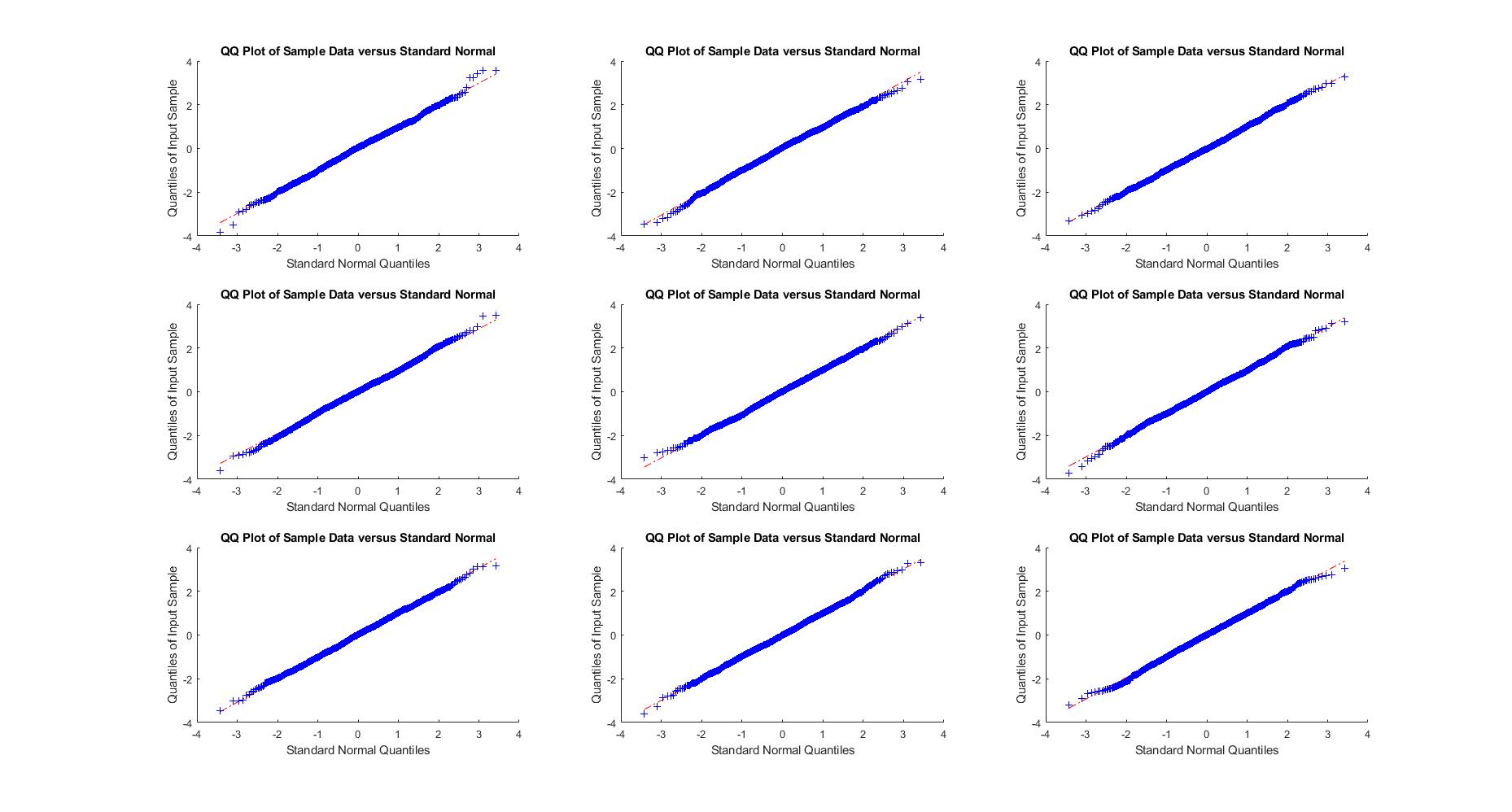
Next, we consider 9 SBMs out of the 81 in Example Example and display in Figure 1 the normal qqplots of the empirical LSS Ln(f)L_{n}(f) after normalization Ln(f)Mean(Ln(f))Std(Ln(f))\frac{L_{n}(f)-Mean(L_{n}(f))}{Std(L_{n}(f))}. These qqplots empirically confirm the asymptotic normality of the LSS.

Refer to caption
Figure 1: qqplots for normalized LSS of 9 different SBMs, test function x2x^{2}
Example.

Same setting except the test function ff is x4x^{4}. Simulation results are shown in Table 2 and Figure 2. The conclusion is similar to that of Example Example.

Asymptotic Empirical maximal absolute difference
Mean of Ln(x4)L_{n}(x^{4}) [Uncaptioned image] [Uncaptioned image] 0.3100
Variance of Ln(x4)L_{n}(x^{4}) [Uncaptioned image] [Uncaptioned image] 0.0065
Table 2: Comparison of the asymptotic mean, variance and their empirical values obtained by Monte Carlo for the LSS Ln(x4)L_{n}(x^{4}). Empirical values use 800800 repetitions.
Refer to caption
Figure 2: qqplots for normalized LSS of 9 different SBMs, test function x4x^{4}

5.2 Experiments on the data-driven matrix H^\hat{H}

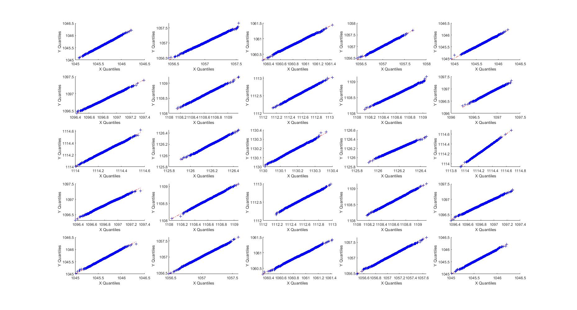
We have also conducted numerical experiments for the data-driven matrix H^\hat{H}. The simulation set-up much follows the one used in Section 3.2. The main purpose is to verify whether the limiting distributions of linear spectral statistics of H^\hat{H} would be the same as those of HH.

Towards this end, we display relative qqplots of linear spectral statistics from HH and H^\hat{H}, respectively. Under distributional identity, qqplots would coincide with the identity line y=xy=x.

Example.

The SBM parameters are as follows:

K=6K=6, α=[0.1,0.15,0.2,0.25,0.1,0.2]\alpha=[0.1,0.15,0.2,0.25,0.1,0.2], N=1000N=1000, Nr=1600N_{r}=1600, P~=(piqj)I+qj11T,\tilde{P}=(p_{i}-q_{j})I+q_{j}11^{T}, where pi=2i110p_{i}=\frac{2i-1}{10}, qj=2j110q_{j}=\frac{2j-1}{10}. Test functions are f1=x4,f_{1}=x^{4}, f2=x5,f_{2}=x^{5}, f3=exp(x).f_{3}=exp(x).

Refer to caption
Figure 3: qqplots of Ln(x4)[H]Ln(x4)[H^]L_{n}(x^{4})[H]-L_{n}(x^{4})[\hat{H}]
Refer to caption
Figure 4: qqplots of Ln(x5)[H]Ln(x5)[H^]L_{n}(x^{5})[H]-L_{n}(x^{5})[\hat{H}]
Refer to caption
Figure 5: qqplots of Ln(exp(x))[H]Ln(exp(x))[H^]L_{n}(exp(x))[H]-L_{n}(exp(x))[\hat{H}]

The empirical qqplots are given in Figure 3 4 5. It can be seen that these qqplots are basically on the line y=xy=x, which gives a good empirical confirmation of Theorem 3.6.

6 Conclusion

In this paper, we consider two applicable renormalizations (Aijpijn)\left(\frac{A_{ij}-p_{ij}}{\sqrt{n}}\right) and (Aijp^ijn)\left(\frac{A_{ij}-\hat{p}_{ij}}{\sqrt{n}}\right) of adjacency matrices of the stochastic block models. The CLTs of linear spectral statistics for both renormalizations are derived. The situations are fundamentally different from the existing literature in the sense that (Aijpijn)\left(\frac{A_{ij}-p_{ij}}{\sqrt{n}}\right) induces a block-Wigner-type matrix whose LSD is no longer guaranteed to be the semicircle law but governed by the so-called quadratic vector equations introduced in [3]. And the CLT for LSS also requires finer tools from the local law estimations. Meanwhile, (Aijp^ijn)\left(\frac{A_{ij}-\hat{p}_{ij}}{\sqrt{n}}\right) is further perturbed by a low rank yet correlated structure, whose non-decaying correlations among the entries increase the difficulty of analysis.

We discuss several directions for future research. First, the CLTs introduced here are still in the dense regime of the stochastic block model. While [24] provides a more subtle analysis of the local law for the Erdős-Rényi model in the sparser regime, it makes a local law for the sparse stochastic block model possible. Thus, the CLT for LSS of SBM in the sparse regime could be doable.

Second, a natural question is that for more general Wigner-type matrices, for instance, when the patterns explore more complex structures, can we get some CLTs or non-CLTs? For instance, if the number of communities for the SBM is growing along with nn or the random graph model is defined via a graphon approach [2][30], then how will the linear spectral statistics behave?

Appendix A Detailed calculations for the proof of Theorem 3.5

In this section, we will show the details of the calculation of the mean function in Section A.1-A.2, covariance function in Section A.3-A.6, proof of normality in Section A.7, and tightness of the process in Section A.8 for the block-Wigner-type matrices HH.

Remark.

Corollary 2.3 will be extensively used in our proof. Since ε>0\varepsilon>0 is arbitrarily small and essentially nεn^{\varepsilon} can be substituted by log(n)k\log(n)^{k} for some large enough kk in these large-deviation bounds. Sometimes we will use nεn^{\varepsilon} for simplicity when it is actually nk0εn^{k_{0}\varepsilon} for some positive integer k0k_{0} which is independent of nn.

Recall that in Section 4, we decompose the mean function TrG(z)TrG(z) into several components. Starting from I1,1I_{1,1} in (17), we need to calculate 𝔼TlG(z)TmG(z)¯\mathbb{E}\underline{T_{l}G(z)T_{m}G(z)} to order 1.

A.1 System of equations for 𝔼G(z)TlG(z)Tm¯\mathbb{E}\underline{G(z)T_{l}G(z)T_{m}}

Proof of Lemma 4.1.

By the identity G(z)=1z(HG(z)I)G(z)=\frac{1}{z}(HG(z)-I), we have

𝔼G(z)TlG(z)Tm¯\displaystyle\mathbb{E}\underline{G(z)T_{l}G(z)T_{m}} =1z𝔼HGTlGTm¯1zTlGTm¯=1z𝔼HGTlGTm¯δlm1z𝔼TlG¯.\displaystyle=\frac{1}{z}\mathbb{E}\underline{HGT_{l}GT_{m}}-\frac{1}{z}\underline{T_{l}GT_{m}}=\frac{1}{z}\mathbb{E}\underline{HGT_{l}GT_{m}}-\delta_{lm}\frac{1}{z}\mathbb{E}\underline{T_{l}G}.

Then by the cumulant expansion formula,

𝔼HGTlGTm¯=1n𝔼ijHij(GTlGTm)ij\displaystyle\mathbb{E}\underline{HGT_{l}GT_{m}}=\frac{1}{n}\mathbb{E}\sum_{ij}H_{ij}(GT_{l}GT_{m})_{ij}
=\displaystyle= ijκij(2)n2𝔼(GTlGTm)jiHij+ijκij(3)2!n5/2𝔼2(GTlGTm)jiHij2\displaystyle\sum_{ij}\frac{\kappa_{ij}^{(2)}}{n^{2}}\mathbb{E}\frac{\partial(GT_{l}GT_{m})_{ji}}{\partial H_{ij}}+\sum_{ij}\frac{\kappa_{ij}^{(3)}}{2!n^{5/2}}\mathbb{E}\frac{\partial^{2}(GT_{l}GT_{m})_{ji}}{\partial H_{ij}^{2}}
+ijκij(4)3!n3𝔼3(GTlGTm)jiHij3+εGTGT,4,\displaystyle+\sum_{ij}\frac{\kappa_{ij}^{(4)}}{3!n^{3}}\mathbb{E}\frac{\partial^{3}(GT_{l}GT_{m})_{ji}}{\partial H_{ij}^{3}}+\varepsilon_{GTGT,4},

where by the cumulant expansion and the trivial bound, the error term satisfies |εGTGT,4|Ci,jsupt|f(3+1)(t)|E[|Hij|3+2]=O(1n)|\varepsilon_{GTGT,4}|\leq C\sum_{i,j}\sup_{t}\left|f^{(3+1)}(t)\right|E\left[|H_{ij}|^{3+2}\right]=O(\frac{1}{\sqrt{n}}) thus minor.

In the meantime, note that when we take derivatives k(GTlGTm)jikHij\frac{\partial^{k}(GT_{l}GT_{m})_{ji}}{\partial^{k}H_{ij}}, the terms with the largest order of magnitude should be the ones with the form ()ii()jj×()(\cdot)_{ii}(\cdot)_{jj}\times(\cdot), which will be of order 1 since G1z||G||\leq\frac{1}{\Im z} and Tl=1,l[K]||T_{l}||=1,\forall l\in[K], so

ijκij(3)2!n5/2𝔼2(GTlGTm)jiHij2=O(1n).\displaystyle\sum_{ij}\frac{\kappa_{ij}^{(3)}}{2!n^{5/2}}\mathbb{E}\frac{\partial^{2}(GT_{l}GT_{m})_{ji}}{\partial H_{ij}^{2}}=O(\frac{1}{\sqrt{n}}). (26)
ijκij(4)3!n3𝔼2(GTlGTm)jiHij2=O(1n).\displaystyle\sum_{ij}\frac{\kappa_{ij}^{(4)}}{3!n^{3}}\mathbb{E}\frac{\partial^{2}(GT_{l}GT_{m})_{ji}}{\partial H_{ij}^{2}}=O(\frac{1}{n}).

It follows that

z𝔼GTlGTm¯+δlm𝔼TlG¯=𝔼HGTlGTm¯=1n𝔼ijHij(GTlGTm)ij\displaystyle z\mathbb{E}\underline{GT_{l}GT_{m}}+\delta_{lm}\mathbb{E}\underline{T_{l}G}=\mathbb{E}\underline{HGT_{l}GT_{m}}=\frac{1}{n}\mathbb{E}\sum_{ij}H_{ij}(GT_{l}GT_{m})_{ij}
=\displaystyle= 1nijκij(2)n𝔼(GTlGTm)jiHij+O(1n)\displaystyle\frac{1}{n}\sum_{ij}\frac{\kappa_{ij}^{(2)}}{n}\mathbb{E}\frac{\partial(GT_{l}GT_{m})_{ji}}{\partial H_{ij}}+O(\frac{1}{\sqrt{n}})
=\displaystyle= 1n2ijκij(2)𝔼[Gji(GTlGTm)ji+Gjj(GTlGTm)ii\displaystyle-\frac{1}{n^{2}}\sum_{ij}\kappa_{ij}^{(2)}\mathbb{E}[G_{ji}(GT_{l}GT_{m})_{ji}+G_{jj}(GT_{l}GT_{m})_{ii}
+(GTlG)ji(GTm)ji+(GTlG)jj(GTm)ii]+O(1n)\displaystyle+(GT_{l}G)_{ji}(GT_{m})_{ji}+(GT_{l}G)_{jj}(GT_{m})_{ii}]+O(\frac{1}{\sqrt{n}})
=\displaystyle= 1n2k1,k2=1KiCk1,jCk2Qk1k2(2)𝔼(Gjj(GTlGTm)ii+(GTlG)jj(GTm)ii)+O(nεn)\displaystyle-\frac{1}{n^{2}}\sum_{k_{1},k_{2}=1}^{K}\sum_{i\in C_{k_{1}},j\in C_{k_{2}}}Q^{(2)}_{k_{1}k_{2}}\mathbb{E}(G_{jj}(GT_{l}GT_{m})_{ii}+(GT_{l}G)_{jj}(GT_{m})_{ii})+O(\frac{n^{\varepsilon}}{\sqrt{n}})
=\displaystyle= k=1KQmk(2)(αkMk(z)𝔼GTlGTm¯+αmMm(z)𝔼GTlGTk¯)+O(nεn).\displaystyle-\sum_{k=1}^{K}Q^{(2)}_{mk}(\alpha_{k}M_{k}(z)\mathbb{E}\underline{GT_{l}GT_{m}}+\alpha_{m}M_{m}(z)\mathbb{E}\underline{GT_{l}GT_{k}})+O(\frac{n^{\varepsilon}}{\sqrt{n}}).

If we adopt the notation

Xm(l):=𝔼GTlGTm¯,X_{m}^{(l)}:=\mathbb{E}\underline{GT_{l}GT_{m}},

then we may rewrite the above system of equations as

(1+1zk=1KQmk(2)αkMk+1zαmMmQmm(2))Xm(l)+1zαmMmk=1,kmKQmk(2)Xk(l)=δml1zαlMl.\displaystyle(1+\frac{1}{z}\sum_{k=1}^{K}Q^{(2)}_{mk}\alpha_{k}M_{k}+\frac{1}{z}\alpha_{m}M_{m}Q^{(2)}_{mm})X_{m}^{(l)}+\frac{1}{z}\alpha_{m}M_{m}\sum_{k=1,k\neq m}^{K}Q^{(2)}_{mk}X_{k}^{(l)}=-\delta_{ml}\frac{1}{z}\alpha_{l}M_{l}. (27)

Now we have the system of equations (21) for vector [𝔼GTlGT1¯,,𝔼GTlGTK¯][\mathbb{E}\underline{GT_{l}GT_{1}},\cdots,\mathbb{E}\underline{GT_{l}GT_{K}}] and the system of equations (22) for matrix (𝔼GTlGTk¯)l,k=1K\big{(}\mathbb{E}\underline{GT_{l}GT_{k}}\big{)}_{l,k=1}^{K}.

Remark.

Further from the QVE (7), for z+z\in\mathbb{C}_{+} and sufficiently bounded away from the spectrum of HH, we have

1Ml(z)=z+m=1KQlm(2)αmMm(z), for all l=1,,K,-\frac{1}{M_{l}(z)}=z+\sum_{m=1}^{K}Q^{(2)}_{lm}\alpha_{m}M_{m}(z),\quad\text{ for all }\quad l=1,\ldots,K,\quad

one can see that for different ll’s. The coefficient matrices are the same, after simplification, we have that the matrix MGTGT(z)=(G(z)TlG(z)Tm¯)l,m=1KM_{GTGT}(z)=\big{(}\underline{G(z)T_{l}G(z)T_{m}}\big{)}_{l,m=1}^{K} adopts this simple explicit form

MGTGT(z)=(Q(2)Diag([1α1M12(z),,1αKMK2(z)]))1,M_{GTGT}(z)=-\big{(}Q^{(2)}-Diag([\frac{1}{\alpha_{1}M_{1}^{2}(z)},\cdots,\frac{1}{\alpha_{K}M_{K}^{2}(z)}]^{\top})\big{)}^{-1}, (28)

which is symmetric and in accordance with the tracial property which leads to

Tr(GTlGTm)=Tr(GTmGTl).Tr(GT_{l}GT_{m})=Tr(GT_{m}GT_{l}).

One may be concerned about the singularity problem. Simply note that |Mj(z)|1|z|,j[K]|M_{j}(z)|\leq\frac{1}{|\Im z|},j\in[K]. Then when |z|2maxk[K]αkj=1KQkj(2),|\Im z|^{2}\geq\max_{k\in[K]}\alpha_{k}\sum_{j=1}^{K}Q^{(2)}_{kj}, the matrix

(Q(2)Diag([1α1M12(z),,1αKMK2(z)]))\big{(}Q^{(2)}-Diag([\frac{1}{\alpha_{1}M_{1}^{2}(z)},\cdots,\frac{1}{\alpha_{K}M_{K}^{2}(z)}]^{\top})\big{)}

becomes diagonal dominant, thus non-singular. Similar things happen when we are near the real axis but also sufficiently bounded away from the edge. Then we can ensure the existence and uniqueness of the solutions of our systems of equations. All we have to pay is to select a larger contour when we apply the Cauchy integral trick to proceed from the trace of the resolvent to the linear spectral statistics. Due to the homogeneity of the coefficient, similar arguments hold for other systems of equations of interest.

Specifically, we introduce the parameter ε0\varepsilon_{0}, s.t. for z\Bε(σ(H^))z\in\mathbb{C}\backslash B_{\varepsilon}(\sigma(\hat{H})), the existence and uniqueness of the solution are guaranteed by the above mechanism.

A.2 Leading term for 1n𝔼i,j=1nκij(2)GiiGjj\frac{1}{n}\mathbb{E}\sum_{i,j=1}^{n}\kappa_{ij}^{(2)}G_{ii}G_{jj} and system of equations for 𝔼Tr(TlG)\mathbb{E}Tr(T_{l}G)

The next task is to identify the leading term of 1n𝔼i,j=1nκij(2)GiiGjj\frac{1}{n}\mathbb{E}\sum_{i,j=1}^{n}\kappa_{ij}^{(2)}G_{ii}G_{jj}. Note that we need to calculate these terms up to the order 11. The problem arises that the trivial upper bound |Gjj(z)mj(z)|1n|G_{jj}(z)-m_{j}(z)|\prec\frac{1}{\sqrt{n}} is far from enough since it only yields 1ni,j=1nκij(2)|GiiGjjmimj|n1/2\frac{1}{n}\sum_{i,j=1}^{n}\kappa_{ij}^{(2)}|G_{ii}G_{jj}-m_{i}m_{j}|\prec n^{1/2}.

Recall the decomposition in (19), we further write

I1,2=\displaystyle I_{1,2}= 1n𝔼k1,k2=1KQk1k2(2)iCk1,jCk2GiiGjj1n𝔼k=1KQkk(2)iCkGll2\displaystyle\frac{1}{n}\mathbb{E}\sum_{k_{1},k_{2}=1}^{K}Q^{(2)}_{k_{1}k_{2}}\sum_{i\in C_{k_{1}},j\in C_{k_{2}}}G_{ii}G_{jj}-\frac{1}{n}\mathbb{E}\sum_{k=1}^{K}Q^{(2)}_{kk}\sum_{i\in C_{k}}G_{ll}^{2} (29)
=\displaystyle= I1,2,1+I1,2,2.\displaystyle I_{1,2,1}+I_{1,2,2}.

where

I1,2,1=\displaystyle I_{1,2,1}= 1n𝔼k1,k2=1KQk1k2(2)iCk1,jCk2GiiGjj=n𝔼k1,k2=1KQk1k2(2)Tk1G¯Tk2G¯.\displaystyle\frac{1}{n}\mathbb{E}\sum_{k_{1},k_{2}=1}^{K}Q^{(2)}_{k_{1}k_{2}}\sum_{i\in C_{k_{1}},j\in C_{k_{2}}}G_{ii}G_{jj}=n\mathbb{E}\sum_{k_{1},k_{2}=1}^{K}Q^{(2)}_{k_{1}k_{2}}\underline{T_{k_{1}}G}\ \underline{T_{k_{2}}G}. (30)

Note that we cannot calculate I1,2,1I_{1,2,1} to the desired order directly.

Simply notice that by local law, we have

𝔼[|Tr(TkG)𝔼Tr(TkG)|2]nε.\displaystyle\mathbb{E}[|Tr(T_{k}G)-\mathbb{E}Tr(T_{k}G)|^{2}]\leq{n^{\varepsilon}}. (31)

By Cauchy-Schwarz inequality it’s easy to see that

𝔼[|(Tr(Tk1G)𝔼Tr(Tk1G))(Tr(Tk2G)𝔼Tr(Tk2G))|]nε.\displaystyle\mathbb{E}[|(Tr(T_{k_{1}}G)-\mathbb{E}Tr(T_{k_{1}}G))(Tr(T_{k_{2}}G)-\mathbb{E}Tr(T_{k_{2}}G))|]\leq{n^{\varepsilon}}. (32)

Then we have

I1,2,1=\displaystyle I_{1,2,1}= n𝔼k1,k2=1KQk1k2(2)Tk1G¯Tk2G¯=nk1,k2=1KQk1k2(2)𝔼Tk1G¯𝔼Tk2G¯+O(nεn).\displaystyle{n}\mathbb{E}\sum_{k_{1},k_{2}=1}^{K}Q^{(2)}_{k_{1}k_{2}}\underline{T_{k_{1}}G}\ \underline{T_{k_{2}}G}={n}\sum_{k_{1},k_{2}=1}^{K}Q^{(2)}_{k_{1}k_{2}}\mathbb{E}\underline{T_{k_{1}}G}\mathbb{E}\underline{T_{k_{2}}G}+O(\frac{n^{\varepsilon}}{n}). (33)

And for I1,2,2I_{1,2,2} we can get the simple formulation

I1,2,2=\displaystyle I_{1,2,2}= 1n𝔼k=1KQkk(2)iCkGii2=k=1KQkk(2)αkMk2+O(nεn).\displaystyle-\frac{1}{n}\mathbb{E}\sum_{k=1}^{K}Q^{(2)}_{kk}\sum_{i\in C_{k}}G_{ii}^{2}=-\sum_{k=1}^{K}Q^{(2)}_{kk}\alpha_{k}M_{k}^{2}+O(\frac{n^{\varepsilon}}{\sqrt{n}}). (34)

In other words, again we have obtained a function of (𝔼(Tr(Tk1G)),𝔼(Tr(Tk2G)))(\mathbb{E}(Tr(T_{k_{1}}G)),\mathbb{E}(Tr(T_{k_{2}}G))) on the RHS, note that the leading order terms of (𝔼(Tr(Tk1G)),𝔼(Tr(Tk2G)))(\mathbb{E}(Tr(T_{k_{1}}G)),\mathbb{E}(Tr(T_{k_{2}}G))), which are of order nn, are known. So this motivates us to derive a system of equations for the subleading order terms of {𝔼Tr(TkG)}k=1K\{\mathbb{E}Tr(T_{k}G)\}_{k=1}^{K}, which are of order 1.

Proof of Lemma 4.2.

By the cumulant expansion formula, we have the following equality for 𝔼Tr(TkG)\mathbb{E}Tr(T_{k}G):

𝔼Tr(TkG)=\displaystyle\mathbb{E}Tr(T_{k}G)= αknz+𝔼1zTr(HGTk)=αknz+𝔼1zij(HijejGTkei)\displaystyle-\frac{\alpha_{k}n}{z}+\mathbb{E}\frac{1}{z}Tr(HGT_{k})=-\frac{\alpha_{k}n}{z}+\mathbb{E}\frac{1}{z}\sum_{ij}(H_{ij}e_{j}^{\prime}GT_{k}e_{i})
=\displaystyle= αknz𝔼1zijκij(2)n[Gjj(GTk)ii+Gji(GTk)ji]+𝔼1zijκij(3)2!n3/22ejGTkeiHij2\displaystyle-\frac{\alpha_{k}n}{z}-\mathbb{E}\frac{1}{z}\sum_{ij}\frac{\kappa_{ij}^{(2)}}{n}[G_{jj}(GT_{k})_{ii}+G_{ji}(GT_{k})_{ji}]+\mathbb{E}\frac{1}{z}\sum_{ij}\frac{\kappa_{ij}^{(3)}}{2!n^{3/2}}\frac{\partial^{2}e_{j}^{\prime}GT_{k}e_{i}}{\partial H_{ij}^{2}}
+𝔼1zijκij(4)3!n23ejGTkeiHij3+εI~1,5\displaystyle+\mathbb{E}\frac{1}{z}\sum_{ij}\frac{\kappa_{ij}^{(4)}}{3!n^{2}}\frac{\partial^{3}e_{j}^{\prime}GT_{k}e_{i}}{\partial H_{ij}^{3}}+\varepsilon_{\tilde{I}_{1,5}}
=\displaystyle= αknz𝔼1zk1,k2=1KiCk1,jCk2,ijκij(2)n[Gjj(GTk)ii+Gji(GTk)ji]\displaystyle-\frac{\alpha_{k}n}{z}-\mathbb{E}\frac{1}{z}\sum_{k_{1},k_{2}=1}^{K}\sum_{i\in C_{k_{1}},j\in C_{k_{2}},i\neq j}\frac{\kappa_{ij}^{(2)}}{n}[G_{jj}(GT_{k})_{ii}+G_{ji}(GT_{k})_{ji}]
+𝔼1zijκij(4)3!n23ejGTkeiHij3+εI~1\displaystyle+\mathbb{E}\frac{1}{z}\sum_{ij}\frac{\kappa_{ij}^{(4)}}{3!n^{2}}\frac{\partial^{3}e_{j}^{\prime}GT_{k}e_{i}}{\partial H_{ij}^{3}}+\varepsilon_{\tilde{I}_{1}}
=\displaystyle= αknzI~1,1I~1,2I~1,4+εI~1,\displaystyle-\frac{\alpha_{k}n}{z}-\tilde{I}_{1,1}-\tilde{I}_{1,2}-\tilde{I}_{1,4}+\varepsilon_{\tilde{I}_{1}},

where εI~1\varepsilon_{\tilde{I}_{1}} consists of higher-order expansions of the formula

εI~1,3\displaystyle\varepsilon_{\tilde{I}_{1},3} =1z𝔼i,jκij(3)2!n3/22[GjjGij(GTk)ii+GjjGii(GTk)ji+GjiGjj(GTk)ii+GjiGji(GTk)ji],\displaystyle=\frac{1}{z}\mathbb{E}\sum_{i,j}\frac{\kappa_{ij}^{(3)}}{2!n^{3/2}}2[G_{jj}G_{ij}(GT_{k})_{ii}+G_{jj}G_{ii}(GT_{k})_{ji}+G_{ji}G_{jj}(GT_{k})_{ii}+G_{ji}G_{ji}(GT_{k})_{ji}],
|εI~1,5|i,jCsupt|f(p+1)(t)|𝔼[|t|p+2]=O(1n).|\varepsilon_{\tilde{I}_{1},5}|\leq\sum_{i,j}C\sup_{t}|f^{(p+1)}(t)|\mathbb{E}[|t|^{p+2}]=O(\frac{1}{\sqrt{n}}).

Then it suffices to show that

εI~1,3l,m=1z𝔼iCl,jCmκij(3)2!n3/22[GjjGij(GTk)ii+GjjGii(GTk)ji+GjiGjj(GTk)ii+GjiGji(GTk)ji]\varepsilon_{\tilde{I}_{1},3}^{l,m}=\frac{1}{z}\mathbb{E}\sum_{i\in C_{l},j\in C_{m}}\frac{\kappa_{ij}^{(3)}}{2!n^{3/2}}2[G_{jj}G_{ij}(GT_{k})_{ii}+G_{jj}G_{ii}(GT_{k})_{ji}+G_{ji}G_{jj}(GT_{k})_{ii}+G_{ji}G_{ji}(GT_{k})_{ji}]

are minor. Let a=[G11,,Gnn]a=[G_{11},\ldots,G_{nn}], bk=[(TkG)11,,(TkG)nn]b_{k}=[(T_{k}G)_{11},\ldots,(T_{k}G)_{nn}].

zεI~1,3l,m\displaystyle z\varepsilon_{\tilde{I}_{1},3}^{l,m}
=\displaystyle= 𝔼iCl,jCmκij(3)2!n3/22[GjjGij(GTk)ii+GjjGii(GTk)ji+GjiGjj(GTk)ii+GjiGji(GTk)ji]\displaystyle\mathbb{E}\sum_{i\in C_{l},j\in C_{m}}\frac{\kappa_{ij}^{(3)}}{2!n^{3/2}}2[G_{jj}G_{ij}(GT_{k})_{ii}+G_{jj}G_{ii}(GT_{k})_{ji}+G_{ji}G_{jj}(GT_{k})_{ii}+G_{ji}G_{ji}(GT_{k})_{ji}]
=\displaystyle= Qlm(3)n3/2(aGbk+a(GTk)a+bkGa)+O(1n)=O(1n).\displaystyle\frac{Q^{(3)}_{lm}}{n^{3/2}}(aGb_{k}^{\top}+a(GT_{k})a^{\top}+b_{k}Ga^{\top})+O(\frac{1}{\sqrt{n}})=O(\frac{1}{\sqrt{n}}).
I~1,1=\displaystyle\tilde{I}_{1,1}= 𝔼1zk1,k2=1KiCk1,jCk2,ijκij(2)nGjj(GTk)ii\displaystyle\mathbb{E}\frac{1}{z}\sum_{k_{1},k_{2}=1}^{K}\sum_{i\in C_{k_{1}},j\in C_{k_{2}},i\neq j}\frac{\kappa_{ij}^{(2)}}{n}G_{jj}(GT_{k})_{ii} (35)
=\displaystyle= 𝔼1zk2=1KiCk,jCk2Qk1k2(2)nTr(Tk2G)Tr(GTk)𝔼1ziCkQkk(2)nGii2\displaystyle\mathbb{E}\frac{1}{z}\sum_{k_{2}=1}^{K}\sum_{i\in C_{k},j\in C_{k_{2}}}\frac{Q^{(2)}_{k_{1}k_{2}}}{n}Tr(T_{k_{2}}G)Tr(GT_{k})-\mathbb{E}\frac{1}{z}\sum_{i\in C_{k}}\frac{Q^{(2)}_{kk}}{n}G_{ii}^{2}
=\displaystyle= 1zk2=1KQk1k2(2)n𝔼Tr(Tk2G)𝔼Tr(GTk)𝔼1zQkk(2)nαknMk2\displaystyle\frac{1}{z}\sum_{k_{2}=1}^{K}\frac{Q^{(2)}_{k_{1}k_{2}}}{n}\mathbb{E}Tr(T_{k_{2}}G)\mathbb{E}Tr(GT_{k})-\mathbb{E}\frac{1}{z}\frac{Q^{(2)}_{kk}}{n}\alpha_{k}nM_{k}^{2}
+1zk2=1KQk1k2(2)n[𝔼Tr(Tk2G)Tr(GTk)𝔼Tr(Tk2G)𝔼Tr(GTk)]\displaystyle+\frac{1}{z}\sum_{k_{2}=1}^{K}\frac{Q^{(2)}_{k_{1}k_{2}}}{n}[\mathbb{E}Tr(T_{k_{2}}G)Tr(GT_{k})-\mathbb{E}Tr(T_{k_{2}}G)\mathbb{E}Tr(GT_{k})]
𝔼1ziCkQkk(2)n[Gii2Mk2(z)].\displaystyle-\mathbb{E}\frac{1}{z}\sum_{i\in C_{k}}\frac{Q^{(2)}_{kk}}{n}[G_{ii}^{2}-M_{k}^{2}(z)].

One may notice that similar to the cases above, we have

|𝔼Tr(Tk2G)Tr(GTk)𝔼Tr(Tk2G)𝔼Tr(GTk)|\displaystyle|\mathbb{E}Tr(T_{k_{2}}G)Tr(GT_{k})-\mathbb{E}Tr(T_{k_{2}}G)\mathbb{E}Tr(GT_{k})|
|𝔼[Tr(Tk2G)|𝔼Tr(Tk2G)][Tr(GTk)𝔼Tr(GTk)]|n2ε,\displaystyle\leq|\mathbb{E}[Tr(T_{k_{2}}G)|-\mathbb{E}Tr(T_{k_{2}}G)][Tr(GT_{k})-\mathbb{E}Tr(GT_{k})]|\leq n^{2\varepsilon},

and

𝔼|Gii2(z)Mk2(z)|=𝔼|Gii(z)Mk(z)||Gii(z)+Mk(z)|nεn(z)2Im(z),iCk,\displaystyle\mathbb{E}|G_{ii}^{2}(z)-M_{k}^{2}(z)|=\mathbb{E}|G_{ii}(z)-M_{k}(z)||G_{ii}(z)+M_{k}(z)|\leq\frac{n^{\varepsilon}}{\sqrt{n\Im(z)}}\frac{2}{Im(z)},\forall i\in C_{k},

thus,

I~1,1=1zk2=1KQk1k2(2)n𝔼Tr(Tk2G)𝔼Tr(GTk)𝔼1zQkk(2)αkMk2+o(1).\tilde{I}_{1,1}=\frac{1}{z}\sum_{k_{2}=1}^{K}\frac{Q^{(2)}_{k_{1}k_{2}}}{n}\mathbb{E}Tr(T_{k_{2}}G)\mathbb{E}Tr(GT_{k})-\mathbb{E}\frac{1}{z}Q^{(2)}_{kk}\alpha_{k}M_{k}^{2}+o(1). (36)

Similarly, we can proceed to I~1,2\tilde{I}_{1,2},

I~1,2=\displaystyle\tilde{I}_{1,2}= 𝔼1zk1,k2=1KiCk1,jCk2,ijκij(2)nGji(GTk)ji\displaystyle\mathbb{E}\frac{1}{z}\sum_{k_{1},k_{2}=1}^{K}\sum_{i\in C_{k_{1}},j\in C_{k_{2}},i\neq j}\frac{\kappa_{ij}^{(2)}}{n}G_{ji}(GT_{k})_{ji} (37)
=\displaystyle= 𝔼1zk1,k2=1KiCk1,jCk2Qk1k2(2)nGji(GTk)ji𝔼1zQkk(2)niCkGii(GTk)ii\displaystyle\mathbb{E}\frac{1}{z}\sum_{k_{1},k_{2}=1}^{K}\sum_{i\in C_{k_{1}},j\in C_{k_{2}}}\frac{Q^{(2)}_{k_{1}k_{2}}}{n}G_{ji}(GT_{k})_{ji}-\mathbb{E}\frac{1}{z}\frac{Q^{(2)}_{kk}}{n}\sum_{i\in C_{k}}G_{ii}(GT_{k})_{ii}
=\displaystyle= 1zk2=1KQkk2(2)𝔼GTk2GTk¯𝔼1zQkk(2)αkMk2+o(1).\displaystyle\frac{1}{z}\sum_{k_{2}=1}^{K}{Q^{(2)}_{kk_{2}}}\mathbb{E}\underline{GT_{k_{2}}GT_{k}}-\mathbb{E}\frac{1}{z}Q^{(2)}_{kk}\alpha_{k}M_{k}^{2}+o(1).
I~1,4\displaystyle\tilde{I}_{1,4} =𝔼1zi,jκij(4)3!n23ejGTkeiHij3=𝔼1ziCk,j,ijκij(4)n2Gii2Gjj2+O(nεn)\displaystyle=\mathbb{E}\frac{1}{z}\sum_{i,j}\frac{\kappa_{ij}^{(4)}}{3!n^{2}}\frac{\partial^{3}e_{j}^{\prime}GT_{k}e_{i}}{\partial H_{ij}^{3}}=\mathbb{E}\frac{1}{z}\sum_{i\in C_{k},j,i\neq j}\frac{\kappa_{ij}^{(4)}}{n^{2}}G_{ii}^{2}G_{jj}^{2}+O(\frac{n^{\varepsilon}}{\sqrt{n}}) (38)
=𝔼1zl=1KiCk,jCl,ijQkl(4)n2Mk2Ml2+O(nεn)=1zl=1KQkl(4)αkαlMk2Ml2+O(nεn).\displaystyle=\mathbb{E}\frac{1}{z}\sum_{l=1}^{K}\sum_{i\in C_{k},j\in C_{l},i\neq j}\frac{Q_{kl}^{(4)}}{n^{2}}M_{k}^{2}M_{l}^{2}+O(\frac{n^{\varepsilon}}{\sqrt{n}})=\frac{1}{z}\sum_{l=1}^{K}{Q_{kl}^{(4)}}\alpha_{k}\alpha_{l}M_{k}^{2}M_{l}^{2}+O(\frac{n^{\varepsilon}}{\sqrt{n}}).

Then we may derive the system of equation for Yk=𝔼Tr(TkG)αknMkY_{k}=\mathbb{E}Tr(T_{k}G)-\alpha_{k}nM_{k},

αknMk+Yk=\displaystyle\alpha_{k}nM_{k}+Y_{k}= αknz1zk2=1KQkk2(2)(αk2nMk2+Yk2)(αknMk+Yk)n\displaystyle-\frac{\alpha_{k}n}{z}-\frac{1}{z}\sum_{k_{2}=1}^{K}Q^{(2)}_{kk_{2}}\frac{(\alpha_{k_{2}}nM_{k_{2}}+Y_{k_{2}})(\alpha_{k}nM_{k}+Y_{k})}{n} (39)
1zk2=1KQkk2(2)𝔼GTk2GTk¯+2Qkk(2)αkMk2z1zl=1KQkl(4)αkαlMk2Ml2.\displaystyle-\frac{1}{z}\sum_{k_{2}=1}^{K}{Q^{(2)}_{kk_{2}}}\mathbb{E}\underline{GT_{k_{2}}GT_{k}}+\frac{2Q^{(2)}_{kk}\alpha_{k}M_{k}^{2}}{z}-\frac{1}{z}\sum_{l=1}^{K}{Q_{kl}^{(4)}}\alpha_{k}\alpha_{l}M_{k}^{2}M_{l}^{2}.

The above equation could be decomposed into two parts, one is of order nn, while the other is of order 1. One may easily verify that the order nn part yields

Mk=1zk2=1KQkk2(2)αk2Mk2Mkz,M_{k}=-\frac{1}{z}-\frac{\sum_{k_{2}=1}^{K}Q^{(2)}_{kk_{2}}\alpha_{k_{2}}M_{k_{2}}M_{k}}{z},

which directly follows from the quadratic vector equation (7), thus canceled.

The order 11 part yields

Yk=\displaystyle Y_{k}= 1zl=1KQkl(2)[αlMlYk+αkMkYl]1zl=1KQkl(2)𝔼GTlGTk¯+2Qkk(2)αkMk2z\displaystyle-\frac{1}{z}\sum_{l=1}^{K}Q^{(2)}_{kl}[\alpha_{l}M_{l}Y_{k}+\alpha_{k}M_{k}Y_{l}]-\frac{1}{z}\sum_{l=1}^{K}{Q^{(2)}_{kl}}\mathbb{E}\underline{GT_{l}GT_{k}}+\frac{2Q^{(2)}_{kk}\alpha_{k}M_{k}^{2}}{z}
1zl=1KQkl(4)αkαlMk2Ml2,\displaystyle-\frac{1}{z}\sum_{l=1}^{K}{Q_{kl}^{(4)}}\alpha_{k}\alpha_{l}M_{k}^{2}M_{l}^{2},

which reformulates into our (23).

A.3 System of equations for Covlm(z1,z2)Cov_{lm}(z_{1},z_{2})

As stated in Section 4, the estimation for Cov(z1,z2)Cov(z_{1},z_{2}) can be decomposed into the summation of the block-wise covariance functions {Covlm(z1,z2)}l,m=1K\{Cov_{lm}(z_{1},z_{2})\}_{l,m=1}^{K}. In this subsection, we will derive the system of equations for {Covlm(z1,z2)}l,m=1K\{Cov_{lm}(z_{1},z_{2})\}_{l,m=1}^{K}.

In this section and thereafter, we will use \langle\cdot\rangle for centered random variables. First, note that for any two random variables XX and YY, we have

𝔼XY=𝔼[X𝔼X][Y𝔼Y]=𝔼X[Y𝔼Y]=𝔼XY,\displaystyle\mathbb{E}\langle X\rangle\langle Y\rangle=\mathbb{E}[X-\mathbb{E}X][Y-\mathbb{E}Y]=\mathbb{E}X[Y-\mathbb{E}Y]=\mathbb{E}X\langle Y\rangle,

then by cumulant expansion formula,

1n2z1𝔼Covlm(z1,z2)=z1𝔼G(z1)Tl¯TmG(z2)¯=z1𝔼G(z1)Tl¯TmG(z2)¯\displaystyle\frac{1}{n^{2}}z_{1}\mathbb{E}Cov_{lm}(z_{1},z_{2})=z_{1}\mathbb{E}\langle\underline{G(z_{1})T_{l}}\rangle\langle\underline{T_{m}G(z_{2})}=z_{1}\mathbb{E}\underline{G(z_{1})T_{l}}\langle\underline{T_{m}G(z_{2})}\rangle (40)
=\displaystyle= 𝔼HG(z1)Tl¯TmG(z2)¯=1n𝔼iCl,jHijGij(z1)TmG(z2)¯\displaystyle\mathbb{E}\underline{HG(z_{1})T_{l}}\langle\underline{T_{m}G(z_{2})}\rangle=\frac{1}{n}\mathbb{E}\sum_{i\in C_{l},j}H_{ij}G_{ij}(z_{1})\langle\underline{T_{m}G(z_{2})}\rangle
=\displaystyle= 1na+b=0𝔼iCl,jκij(a+b+1)na+b+12a!b!aGij(z1)bTmG(z2)¯Hij(a+b)\displaystyle\frac{1}{n}\sum_{a+b=0}^{\infty}\mathbb{E}\sum_{i\in C_{l},j}\frac{\kappa^{(a+b+1)}_{ij}}{n^{\frac{a+b+1}{2}}a!b!}\frac{\partial^{a}G_{ij}(z_{1})\partial^{b}\langle\underline{T_{m}G(z_{2})}\rangle}{\partial H_{ij}^{(a+b)}}
=\displaystyle= a+b=05I2,(a,b)+εI2.\displaystyle\sum_{a+b=0}^{5}I_{2,(a,b)}+\varepsilon_{I_{2}}.

Now we proceed to the detailed treatments for the terms {I2,(a,b)}a+b=13\{I_{2,(a,b)}\}_{a+b=1}^{3}. It can be shown that a+b=45I2,(a,b)\sum_{a+b=4}^{5}I_{2,(a,b)} are minor via similar calculations, the details for calculating a+b=45I2,(a,b)\sum_{a+b=4}^{5}I_{2,(a,b)} are tedious and of minor importance thus omitted here and in the proof of (10).

Proof of (10).
I2,(1,0)\displaystyle I_{2,(1,0)}
=\displaystyle= 1n𝔼k1=1KQlk1(2)n[Tr(TlG(z1)Tk1G(z1))+Tr(TlG(z1))Tr(Tk1G(z1))]TmG(z2)¯\displaystyle-\frac{1}{n}\mathbb{E}\sum_{k_{1}=1}^{K}\frac{Q^{(2)}_{lk_{1}}}{n}[Tr(T_{l}G(z_{1})T_{k_{1}}G(z_{1}))+Tr(T_{l}G(z_{1}))Tr(T_{k_{1}}G(z_{1}))]\langle\underline{T_{m}G(z_{2})}\rangle
+2Qll(2)n2𝔼iCl[Gii2(z1)Ml2(z1)]TmG(z2)¯\displaystyle+\frac{2Q^{(2)}_{ll}}{n^{2}}\mathbb{E}\sum_{i\in C_{l}}[G_{ii}^{2}(z_{1})-M_{l}^{2}(z_{1})]\langle\underline{T_{m}G(z_{2})}\rangle
=\displaystyle= 𝔼k1=1KQlk1(2)nTlG(z1)Tk1G(z1)¯TmG(z2)¯𝔼k1=1KQlk1(2)TlG(z1)¯Tk1G(z1)¯TmG(z2)¯\displaystyle-\mathbb{E}\sum_{k_{1}=1}^{K}\frac{Q^{(2)}_{lk_{1}}}{n}\langle\underline{T_{l}G(z_{1})T_{k_{1}}G(z_{1})}\rangle\langle\underline{T_{m}G(z_{2})}\rangle-\mathbb{E}\sum_{k_{1}=1}^{K}Q^{(2)}_{lk_{1}}\langle\underline{T_{l}G(z_{1})}\rangle\ \langle\underline{T_{k_{1}}G(z_{1})}\rangle\ \langle\underline{T_{m}G(z_{2})}\rangle
𝔼k1=1KQlk1(2)TlG(z1)¯Tk1G(z1)¯TmG(z2)¯𝔼k1=1KQlk1(2)TlG(z1)¯Tk1G(z1)¯TmG(z2)¯\displaystyle-\mathbb{E}\sum_{k_{1}=1}^{K}Q^{(2)}_{lk_{1}}\langle\underline{T_{l}G(z_{1})}\rangle\underline{T_{k_{1}}G(z_{1})}\langle\underline{T_{m}G(z_{2})}\rangle-\mathbb{E}\sum_{k_{1}=1}^{K}Q^{(2)}_{lk_{1}}\underline{T_{l}G(z_{1})}\langle\underline{T_{k_{1}}G(z_{1})}\rangle\langle\underline{T_{m}G(z_{2})}\rangle
+O(nεn5/2)\displaystyle+O(\frac{n^{\varepsilon}}{n^{5/2}})
=\displaystyle= k1=1KQlk1(2)αk1Mk1(z1)Covlm(z1,z2)k1=1KQlk1(2)αlMl(z1)Covk1m(z1,z2)+O(nεn5/2).\displaystyle-\sum_{k_{1}=1}^{K}Q^{(2)}_{lk_{1}}\alpha_{k_{1}}M_{k_{1}}(z_{1})Cov_{lm}(z_{1},z_{2})-\sum_{k_{1}=1}^{K}Q^{(2)}_{lk_{1}}\alpha_{l}M_{l}(z_{1})Cov_{k_{1}m}(z_{1},z_{2})+O(\frac{n^{\varepsilon}}{n^{5/2}}).
I2,(0,1)\displaystyle I_{2,(0,1)}
=\displaystyle= 1n𝔼k1=1KiCl,jCk1Qlk1(2)nGij(z1)1nkCm(Gkj(z2)Gik(z2)+Gki(z2)Gjk(z2))\displaystyle-\frac{1}{n}\mathbb{E}\sum_{k_{1}=1}^{K}\sum_{i\in C_{l},j\in C_{k_{1}}}\frac{Q^{(2)}_{lk_{1}}}{n}G_{ij}(z_{1})\frac{1}{n}\sum_{k\in C_{m}}(G_{kj}(z_{2})G_{ik}(z_{2})+G_{ki}(z_{2})G_{jk}(z_{2}))
+1n𝔼iClQll(2)nGii(z1)1nkCm(Gki(z2)Gik(z2)+Gki(z2)Gik(z2))\displaystyle+\frac{1}{n}\mathbb{E}\sum_{i\in C_{l}}\frac{Q^{(2)}_{ll}}{n}G_{ii}(z_{1})\frac{1}{n}\sum_{k\in C_{m}}(G_{ki}(z_{2})G_{ik}(z_{2})+G_{ki}(z_{2})G_{ik}(z_{2}))
=\displaystyle= 𝔼k1=1KiCl,jCk12Qlk1(2)n3Gij(z1)(GTmG)ij(z2)+𝔼iCl2Qll(2)n3Gii(z1)(GTmG)ii(z2)\displaystyle-\mathbb{E}\sum_{k_{1}=1}^{K}\sum_{i\in C_{l},j\in C_{k_{1}}}\frac{2Q^{(2)}_{lk_{1}}}{n^{3}}G_{ij}(z_{1})(GT_{m}G)_{ij}(z_{2})+\mathbb{E}\sum_{i\in C_{l}}\frac{2Q^{(2)}_{ll}}{n^{3}}G_{ii}(z_{1})(GT_{m}G)_{ii}(z_{2})
=\displaystyle= k1=1K2Qlk1(2)n2𝔼G(z1)TlG(z2)TmG(z2)Tk1¯+2Qll(2)n2Ml(z1)𝔼(TlGTmG)(z2)¯+O(nεn5/2).\displaystyle-\sum_{k_{1}=1}^{K}\frac{2Q^{(2)}_{lk_{1}}}{n^{2}}\mathbb{E}\underline{G(z_{1})T_{l}G(z_{2})T_{m}G(z_{2})T_{k_{1}}}+\frac{2Q^{(2)}_{ll}}{n^{2}}M_{l}(z_{1})\mathbb{E}\underline{(T_{l}GT_{m}G)(z_{2})}+O(\frac{n^{\varepsilon}}{n^{5/2}}).

We claim that in I2,(1,0)I_{2,(1,0)} both 1n𝔼TlG(z1)Tk1G(z1)¯TmG(z2)¯\frac{1}{n}\mathbb{E}\langle\underline{T_{l}G(z_{1})T_{k_{1}}G(z_{1})}\rangle\langle\underline{T_{m}G(z_{2})}\rangle and the triple-product term 𝔼TlG(z1)¯Tk1G(z1)¯TmG(z2)¯\mathbb{E}\langle\underline{T_{l}G(z_{1})}\rangle\ \langle\underline{T_{k_{1}}G(z_{1})}\rangle\ \langle\underline{T_{m}G(z_{2})}\rangle will be the minor terms. The second one is of order nεn3\frac{n^{\varepsilon}}{n^{3}} by Cauchy inequality, thus minor. The first one, however, requires a little bit effort.

To get an sufficient upper bound for 1n𝔼TlG(z1)Tk1G(z1)¯TmG(z2)¯\frac{1}{n}\mathbb{E}\langle\underline{T_{l}G(z_{1})T_{k_{1}}G(z_{1})}\rangle\langle\underline{T_{m}G(z_{2})}\rangle, we only need to show that 𝔼|Tk1G(z)Tk2G(z)¯|2\mathbb{E}|\langle\underline{T_{k_{1}}G(z)T_{k_{2}}G(z)}\rangle|^{2} is of order O(nt)O(n^{-t}) for some t>0t>0. By intuition from the classic Wigner matrix, the essential order for 𝔼|Tk1G(z)Tk2G(z)¯|2\mathbb{E}|\langle\underline{T_{k_{1}}G(z)T_{k_{2}}G(z)}\rangle|^{2} should be O(n2)O(n^{-2}). We refer to the Section A.4 for the details.

Also, I2,(0,1)I_{2,(0,1)} gives rise to the quantities 𝔼G(z1)TlG(z2)TmG(z2)Tk1¯\mathbb{E}\underline{G(z_{1})T_{l}G(z_{2})T_{m}G(z_{2})T_{k_{1}}} which will be treated in Section A.5 and 𝔼G(z2)TlG(z2)Tm¯\mathbb{E}\underline{G(z_{2})T_{l}G(z_{2})T_{m}} which has already been studied in Section A.1.

I2,(2,0)=\displaystyle I_{2,(2,0)}= 1n𝔼iCl,jκij(3)n3/2[(Gij(z1))3+3Gii(z1)Gjj(z1)Gij(z1)]TmG(z2)¯\displaystyle\frac{1}{n}\mathbb{E}\sum_{i\in C_{l},j}\frac{\kappa_{ij}^{(3)}}{n^{3/2}}[(G_{ij}(z_{1}))^{3}+3G_{ii}(z_{1})G_{jj}(z_{1})G_{ij}(z_{1})]\langle\underline{T_{m}G(z_{2})}\rangle (41)
=\displaystyle= 1n𝔼iCl,jκij(3)n3/2[3Gii(z1)Gjj(z1)Gij(z1)]TmG(z2)¯+O(nεn3).\displaystyle\frac{1}{n}\mathbb{E}\sum_{i\in C_{l},j}\frac{\kappa_{ij}^{(3)}}{n^{3/2}}[3G_{ii}(z_{1})G_{jj}(z_{1})G_{ij}(z_{1})]\langle\underline{T_{m}G(z_{2})}\rangle+O(\frac{n^{\varepsilon}}{n^{3}}).

Note that one argument for higher-order expansion terms in the cumulant expansion that we will use over and over again is that we can ignore the diagonal terms in many situations since there are only nn diagonal terms which are at most O(1)O(1) each. To be more specific,

nεnd+12+2|m=1ndGmmHmmd|nεnd+12+1Cnεn(d+3)/2=o(n2),d=2,3,\displaystyle\frac{n^{\varepsilon}}{n^{\frac{d+1}{2}+2}}|\sum_{m=1}^{n}\frac{\partial^{d}G_{mm}}{\partial H_{mm}^{d}}|\leq\frac{n^{\varepsilon}}{n^{\frac{d+1}{2}+1}}\leq\frac{C^{\prime}n^{\varepsilon}}{n^{(d+3)/2}}=o(n^{-2}),d=2,3,

then w.l.o.g. we can ignore the diagonal terms here. Further, because TmG¯\langle\underline{T_{m}G}\rangle is O(nεn)O_{\prec}(\frac{n^{\varepsilon}}{n}), we only need to show that 1n𝔼iCl,jCmκij(3)n3/2GijGiiGjj=o(1n1+t)\frac{1}{n}\mathbb{E}\sum_{i\in C_{l},j\in C_{m}}\frac{\kappa_{ij}^{(3)}}{n^{3/2}}G_{ij}G_{ii}G_{jj}=o(\frac{1}{n^{1+t}}) for any t>0t>0 to ensure that I2,(2,0)I_{2,(2,0)} is vanishing.

Note that the trivial bounds for GijGiiGjjG_{ij}G_{ii}G_{jj} will not be sufficient. The trick here is to apply the cumulant expansion formula one more time to get certain equation of 1n𝔼iCl,jCmκij(3)n3/2GijGiiGjj=o(1n1+t)\frac{1}{n}\mathbb{E}\sum_{i\in C_{l},j\in C_{m}}\frac{\kappa_{ij}^{(3)}}{n^{3/2}}G_{ij}G_{ii}G_{jj}=o(\frac{1}{n^{1+t}}), hence the sufficient bounds.

By cumulant expansion, we have

1n𝔼iCl,jCmκij(3)n3/2GijGiiGjj=Qlm(3)n5/2𝔼iCl,jCmGijGiiGjjQlm(3)n5/2𝔼iClδlmGii3\displaystyle\frac{1}{n}\mathbb{E}\sum_{i\in C_{l},j\in C_{m}}\frac{\kappa_{ij}^{(3)}}{n^{3/2}}G_{ij}G_{ii}G_{jj}=\frac{Q^{(3)}_{lm}}{n^{5/2}}\mathbb{E}\sum_{i\in C_{l},j\in C_{m}}G_{ij}G_{ii}G_{jj}-\frac{Q^{(3)}_{lm}}{n^{5/2}}\mathbb{E}\sum_{i\in C_{l}}\delta_{lm}G_{ii}^{3} (42)
=\displaystyle= Qlm(3)n5/2𝔼1ziCl,jCmkHikGkjGiiGjj+O(n3/2)\displaystyle\frac{Q^{(3)}_{lm}}{n^{5/2}}\mathbb{E}\frac{1}{z}\sum_{i\in C_{l},j\in C_{m}}\sum_{k}H_{ik}G_{kj}G_{ii}G_{jj}+O(n^{-3/2})
=\displaystyle= Qlm(3)n5/2𝔼1ziCl,jCmkκik(2)n(GkjGiiGjj)Hik+Qlm(3)n5/2𝔼1ziCl,jCmkκik(3)2!n3/22(GkjGiiGjj)Hik2\displaystyle\frac{Q^{(3)}_{lm}}{n^{5/2}}\mathbb{E}\frac{1}{z}\sum_{i\in C_{l},j\in C_{m}}\sum_{k}\frac{\kappa^{(2)}_{ik}}{n}\frac{\partial(G_{kj}G_{ii}G_{jj})}{\partial H_{ik}}+\frac{Q^{(3)}_{lm}}{n^{5/2}}\mathbb{E}\frac{1}{z}\sum_{i\in C_{l},j\in C_{m}}\sum_{k}\frac{\kappa^{(3)}_{ik}}{2!n^{3/2}}\frac{\partial^{2}(G_{kj}G_{ii}G_{jj})}{\partial H_{ik}^{2}}
+Qlm(3)n5/2𝔼1ziCl,jCmkκik(4)3!n23(GkjGiiGjj)Hik3+O(n3/2).\displaystyle+\frac{Q^{(3)}_{lm}}{n^{5/2}}\mathbb{E}\frac{1}{z}\sum_{i\in C_{l},j\in C_{m}}\sum_{k}\frac{\kappa^{(4)}_{ik}}{3!n^{2}}\frac{\partial^{3}(G_{kj}G_{ii}G_{jj})}{\partial H_{ik}^{3}}+O(n^{-3/2}).

Then the problem becomes to derive bounds for the terms

Qlm(3)n5/2𝔼1ziCl,jCmkκik(2)n(GkjGiiGjj)Hik\displaystyle\frac{Q^{(3)}_{lm}}{n^{5/2}}\mathbb{E}\frac{1}{z}\sum_{i\in C_{l},j\in C_{m}}\sum_{k}\frac{\kappa^{(2)}_{ik}}{n}\frac{\partial(G_{kj}G_{ii}G_{jj})}{\partial H_{ik}}
=\displaystyle= Qlm(3)n7/2𝔼1ziCl,jCmk1=1KkCk1κik(2)[(GikGjk+GijGkk)GiiGjj\displaystyle\frac{Q^{(3)}_{lm}}{n^{7/2}}\mathbb{E}\frac{1}{z}\sum_{i\in C_{l},j\in C_{m}}\sum_{k_{1}=1}^{K}\sum_{k\in C_{k_{1}}}\kappa_{ik}^{(2)}[-(G_{ik}G_{jk}+G_{ij}G_{kk})G_{ii}G_{jj}
2GkjGiiGikGjj2GkjGiiGijGkj]\displaystyle-2G_{kj}G_{ii}G_{ik}G_{jj}-2G_{kj}G_{ii}G_{ij}G_{kj}]
=\displaystyle= Qlm(3)n7/2𝔼1ziCl,jCmk1=1KQlk1(2)Tr(Tk1G)GijGiiGjj+O(Kn3/2)\displaystyle-\frac{Q^{(3)}_{lm}}{n^{7/2}}\mathbb{E}\frac{1}{z}\sum_{i\in C_{l},j\in C_{m}}\sum_{k_{1}=1}^{K}Q^{(2)}_{lk_{1}}Tr(T_{k_{1}}G)G_{ij}G_{ii}G_{jj}+O(\frac{K}{n^{3/2}})
=\displaystyle= Qlm(3)n7/2zk1=1KQlk1(2)𝔼Tr(Tk1G)𝔼iCl,jCmGijGiiGjj+O(Knεn3/2).\displaystyle-\frac{Q^{(3)}_{lm}}{n^{7/2}z}\sum_{k_{1}=1}^{K}Q^{(2)}_{lk_{1}}\mathbb{E}Tr(T_{k_{1}}G)\mathbb{E}\sum_{i\in C_{l},j\in C_{m}}G_{ij}G_{ii}G_{jj}+O(\frac{Kn^{\varepsilon}}{n^{3/2}}).

In the meantime,

Qlm(3)n5/2𝔼1ziCl,jCmkκik(3)n3/22(GkjGiiGjj)Hik2\displaystyle\frac{Q^{(3)}_{lm}}{n^{5/2}}\mathbb{E}\frac{1}{z}\sum_{i\in C_{l},j\in C_{m}}\sum_{k}\frac{\kappa_{ik}^{(3)}}{n^{3/2}}\frac{\partial^{2}(G_{kj}G_{ii}G_{jj})}{\partial H_{ik}^{2}}
=\displaystyle= {at least two of i,j,k would be the same}+{i,j,k are mutually different}\displaystyle\sum\{\text{at least two of }i,j,k\text{ would be the same}\}+\sum\{i,j,k\text{ are mutually different}\}
=\displaystyle= O(nεn3/2),\displaystyle O(\frac{n^{\varepsilon}}{n^{3/2}}),

while the trivial upper bound is already sufficient for the 44-th order term

Qlm(3)n5/2𝔼1ziCl,jCmkκik(4)n23(GkjGiiGjj)Hik3=O(n3/2).\displaystyle\frac{Q^{(3)}_{lm}}{n^{5/2}}\mathbb{E}\frac{1}{z}\sum_{i\in C_{l},j\in C_{m}}\sum_{k}\frac{\kappa^{(4)}_{ik}}{n^{2}}\frac{\partial^{3}(G_{kj}G_{ii}G_{jj})}{\partial H_{ik}^{3}}=O(n^{-3/2}).

Thus, from above estimations we know

1n𝔼iCl,jCmκij(3)n3/2GijGiiGjj\displaystyle\frac{1}{n}\mathbb{E}\sum_{i\in C_{l},j\in C_{m}}\frac{\kappa^{(3)}_{ij}}{n^{3/2}}G_{ij}G_{ii}G_{jj} (43)
=\displaystyle= Qlm(3)n5/2zk1=1KQlk1(2)𝔼Tr(Tk1G)n𝔼iCl,jCmGijGiiGjj+O(Knεn3/2),\displaystyle-\frac{Q^{(3)}_{lm}}{n^{5/2}z}\sum_{k_{1}=1}^{K}Q^{(2)}_{lk_{1}}\mathbb{E}\frac{Tr(T_{k_{1}}G)}{n}\mathbb{E}\sum_{i\in C_{l},j\in C_{m}}G_{ij}G_{ii}G_{jj}+O(\frac{Kn^{\varepsilon}}{n^{3/2}}),

instantly we come to the conclusion that

𝔼iCl,jCmGijGiiGjj=O(Kn1+ε).\mathbb{E}\sum_{i\in C_{l},j\in C_{m}}G_{ij}G_{ii}G_{jj}=O(Kn^{1+\varepsilon}). (44)

Thus, 1n𝔼iCl,jCmκij(3)n3/2GijGiiGjj\frac{1}{n}\mathbb{E}\sum_{i\in C_{l},j\in C_{m}}\frac{\kappa^{(3)}_{ij}}{n^{3/2}}G_{ij}G_{ii}G_{jj} is minor and I2,(2,0)I_{2,(2,0)} is also minor.

I2,(1,1)\displaystyle I_{2,(1,1)}
=\displaystyle= 1n𝔼iCl,j2κij(3)2!n3/2(Gij2(z1)+Gii(z1)Gjj(z1))1nkCm[Gkj(z2)Gik(z2)+Gki(z2)Gjk(z2)]\displaystyle\frac{1}{n}\mathbb{E}\sum_{i\in C_{l},j}\frac{2\kappa_{ij}^{(3)}}{2!n^{3/2}}(G_{ij}^{2}(z_{1})+G_{ii}(z_{1})G_{jj}(z_{1}))\frac{1}{n}\sum_{k\in C_{m}}[G_{kj}(z_{2})G_{ik}(z_{2})+G_{ki}(z_{2})G_{jk}(z_{2})]
=\displaystyle= 1n7/2k1=1KiCl,jCk12Qlk1(3)Gii(z1)Gjj(z1)(GTmG)ij(z2)+O(nεn5/2).\displaystyle\frac{1}{n^{7/2}}\sum_{k_{1}=1}^{K}\sum_{i\in C_{l},j\in C_{k_{1}}}2Q^{(3)}_{lk_{1}}G_{ii}(z_{1})G_{jj}(z_{1})(GT_{m}G)_{ij}(z_{2})+O(\frac{n^{\varepsilon}}{n^{5/2}}).

Simply note that |Gii(z)||1z||G_{ii}(z)|\leq|\frac{1}{\Im z}|, G(z)|1z|||G(z)||\leq|\frac{1}{\Im z}| and Tm=1||T_{m}||=1, we have

𝔼1n7/2iCl,jCk1Qlk1(3)Gii(z1)Gjj(z1)(GTmG)ij(z2)\displaystyle\mathbb{E}\frac{1}{n^{7/2}}\sum_{i\in C_{l},j\in C_{k_{1}}}Q^{(3)}_{lk_{1}}G_{ii}(z_{1})G_{jj}(z_{1})(GT_{m}G)_{ij}(z_{2}) (45)
=\displaystyle= 𝔼1n7/2iCl,jCk1Qlk1(3)diag(G(z1))×(GTmG)(z2)×diag(G(z1))\displaystyle\mathbb{E}\frac{1}{n^{7/2}}\sum_{i\in C_{l},j\in C_{k_{1}}}Q^{(3)}_{lk_{1}}diag(G(z_{1}))\times(GT_{m}G)(z_{2})\times diag(G(z_{1}))
=\displaystyle= O(n5/2).\displaystyle O(n^{-5/2}).

Further,

I2,(0,2)\displaystyle I_{2,(0,2)}
=\displaystyle= 𝔼k1=1KiCl,jCk1κlk1(3)n7/2Gij(z1)kCm(GkjGijGik+GkjGiiGjk+GkiGjjGik+GkiGjiGjk)\displaystyle-\mathbb{E}\sum_{k_{1}=1}^{K}\sum_{i\in C_{l},j\in C_{k_{1}}}\frac{\kappa_{lk_{1}}^{(3)}}{n^{7/2}}G_{ij}(z_{1})\sum_{k\in C_{m}}(G_{kj}G_{ij}G_{ik}+G_{kj}G_{ii}G_{jk}+G_{ki}G_{jj}G_{ik}+G_{ki}G_{ji}G_{jk})
=\displaystyle= 𝔼k1=1KiCl,jCk1κlk1(3)n7/2Gij(z1)[(GTmG)ijGij+(GTmG)jjGii+(GTmG)iiGjj\displaystyle-\mathbb{E}\sum_{k_{1}=1}^{K}\sum_{i\in C_{l},j\in C_{k_{1}}}\frac{\kappa_{lk_{1}}^{(3)}}{n^{7/2}}G_{ij}(z_{1})[(GT_{m}G)_{ij}G_{ij}+(GT_{m}G)_{jj}G_{ii}+(GT_{m}G)_{ii}G_{jj}
+(GTmG)jiGji](z2)\displaystyle+(GT_{m}G)_{ji}G_{ji}](z_{2})
=\displaystyle= O(nεn5/2),\displaystyle O(\frac{n^{\varepsilon}}{n^{5/2}}),

where we use the fact that

iCl,jCk1Qlk1(3)n7/2Gii(GTmG)ij(GTmG)jj|=Qlk1(3)n7/2(diag(TlG)×(GTmG)×diag(Tk1GTmG))\displaystyle\sum_{i\in C_{l},j\in C_{k_{1}}}\frac{Q^{(3)}_{lk_{1}}}{n^{7/2}}G_{ii}(GT_{m}G)_{ij}(GT_{m}G)_{jj}|=\frac{Q^{(3)}_{lk_{1}}}{n^{7/2}}(diag(T_{l}G)\times(GT_{m}G)\times diag(T_{k_{1}}GT_{m}G))
=\displaystyle= O(1n5/2).\displaystyle O(\frac{1}{n^{5/2}}).
I2,(3,0)=\displaystyle I_{2,(3,0)}= 1n𝔼k1=1KiCl,jCk1,ijQlk1(4)n2(Gij4+6Gij2GiiGjj+Gii2Gjj2)TmG(z2)¯\displaystyle\frac{1}{n}\mathbb{E}\sum_{k_{1}=1}^{K}\sum_{i\in C_{l},j\in C_{k_{1}},i\neq j}\frac{Q^{(4)}_{lk_{1}}}{n^{2}}(G_{ij}^{4}+6G_{ij}^{2}G_{ii}G_{jj}+G_{ii}^{2}G_{jj}^{2})\langle\underline{T_{m}G(z_{2})}\rangle
=\displaystyle= k1=1KiCl,jCk1,ijQlk1(4)n3Ml2Mk12𝔼TmG(z2)¯\displaystyle\sum_{k_{1}=1}^{K}\sum_{i\in C_{l},j\in C_{k_{1}},i\neq j}\frac{Q^{(4)}_{lk_{1}}}{n^{3}}M_{l}^{2}M_{k_{1}}^{2}\mathbb{E}\langle\underline{T_{m}G(z_{2})}\rangle
+k1=1KiCl,jCk1,ijQlk1(4)n3𝔼(Gii2Gjj2Ml2Mk12)TmG(z2)¯+O(nεn3)\displaystyle+\sum_{k_{1}=1}^{K}\sum_{i\in C_{l},j\in C_{k_{1}},i\neq j}\frac{Q^{(4)}_{lk_{1}}}{n^{3}}\mathbb{E}(G_{ii}^{2}G_{jj}^{2}-M_{l}^{2}M_{k_{1}}^{2})\langle\underline{T_{m}G(z_{2})}\rangle+O(\frac{n^{\varepsilon}}{n^{3}})
=\displaystyle= O(n2εn5/2).\displaystyle O(\frac{n^{2\varepsilon}}{n^{5/2}}).
I2,(2,1)=\displaystyle I_{2,(2,1)}= 3n𝔼iCl,j2κij(4)3!n2[Gij3(z1)+Gij(z1)Gii(z1)Gjj(z1)]\displaystyle-\frac{3}{n}\mathbb{E}\sum_{i\in C_{l},j}\frac{2\kappa_{ij}^{(4)}}{3!n^{2}}[G_{ij}^{3}(z_{1})+G_{ij}(z_{1})G_{ii}(z_{1})G_{jj}(z_{1})]
×3nkCm[Gki(z2)Gjk(z2)+Gkj(z2)Gik(z2)]\displaystyle\times\frac{3}{n}\sum_{k\in C_{m}}[G_{ki}(z_{2})G_{jk}(z_{2})+G_{kj}(z_{2})G_{ik}(z_{2})]
=\displaystyle= 3n2𝔼iCl,j2κij(4)n2[Gij3(z1)+Gij(z1)Gii(z1)Gjj(z1)]2(GTmG)ij(z2)\displaystyle-\frac{3}{n^{2}}\mathbb{E}\sum_{i\in C_{l},j}\frac{2\kappa_{ij}^{(4)}}{n^{2}}[G_{ij}^{3}(z_{1})+G_{ij}(z_{1})G_{ii}(z_{1})G_{jj}(z_{1})]2(GT_{m}G)_{ij}(z_{2})
=\displaystyle= O(nεn5/2).\displaystyle O(\frac{n^{\varepsilon}}{n^{5/2}}).
I2,(1,2)=\displaystyle I_{2,(1,2)}= 3n𝔼iCl,j2κij(4)3!n2[Gij2(z1)+Gii(z1)Gjj(z1)]\displaystyle-\frac{3}{n}\mathbb{E}\sum_{i\in C_{l},j}\frac{2\kappa^{(4)}_{ij}}{3!n^{2}}[G_{ij}^{2}(z_{1})+G_{ii}(z_{1})G_{jj}(z_{1})]
×1n[(GTmG)ijGij+(GTmG)iiGjj+(GTmG)jiGji+(GTmG)jjGii](z2)\displaystyle\times\frac{1}{n}[(GT_{m}G)_{ij}G_{ij}+(GT_{m}G)_{ii}G_{jj}+(GT_{m}G)_{ji}G_{ji}+(GT_{m}G)_{jj}G_{ii}](z_{2})
=\displaystyle= 𝔼k=1KQlk(4)n2[αkMl(z1)Mk(z1)(GTmGTl)(z2)¯Mk(z2)\displaystyle-\mathbb{E}\sum_{k=1}^{K}\frac{Q^{(4)}_{lk}}{n^{2}}[\alpha_{k}M_{l}(z_{1})M_{k}(z_{1})\underline{(GT_{m}GT_{l})(z_{2})}M_{k}(z_{2})
+αlMl(z1)Mk(z1)(GTmGTk)(z2)¯Ml(z2)]+O(nεn5/2).\displaystyle+\alpha_{l}M_{l}(z_{1})M_{k}(z_{1})\underline{(GT_{m}GT_{k})(z_{2})}M_{l}(z_{2})]+O(\frac{n^{\varepsilon}}{n^{5/2}}).
I2,(0,3)\displaystyle I_{2,(0,3)}
=\displaystyle= 1n𝔼iCl,jκij(4)n2Gij(z1)1n[Gij2(G2)jj+Gij2(G2)jj+GiiGjj(G2)ij+GiiGji(G2)jj\displaystyle-\frac{1}{n}\mathbb{E}\sum_{i\in C_{l},j}\frac{\kappa_{ij}^{(4)}}{n^{2}}G_{ij}(z_{1})\frac{1}{n}[G_{ij}^{2}(G^{2})_{jj}+G_{ij}^{2}(G^{2})_{jj}+G_{ii}G_{jj}(G^{2})_{ij}+G_{ii}G_{ji}(G^{2})_{jj}
+GjjGij(G2)ii+GjjGii(G2)ji+GjiGjj(G2)ii+Gji2(G2)ji](z2)\displaystyle+G_{jj}G_{ij}(G^{2})_{ii}+G_{jj}G_{ii}(G^{2})_{ji}+G_{ji}G_{jj}(G^{2})_{ii}+G_{ji}^{2}(G^{2})_{ji}](z_{2})
=\displaystyle= O(nεn5/2).\displaystyle O(\frac{n^{\varepsilon}}{n^{5/2}}).

Similarly, we can derive that a+b=45I2,(a,b)\sum_{a+b=4}^{5}I_{2,(a,b)} is also minor. Further note that

εI2=1ni,jCsupt|f(5+1)(t)|E[|ξ|5+2]=O(1n5/2).\displaystyle\varepsilon_{I_{2}}=\frac{1}{n}\sum_{i,j}C\sup_{t}|f^{(5+1)}(t)|E[|\xi|^{5+2}]=O(\frac{1}{n^{5/2}}).

To conclude, the covariance function {Covlm(z1,z2)}l,m[K]\{Cov_{lm}(z_{1},z_{2})\}_{l,m\in[K]} satisfies the following system of equations to order 1

z1Covlm(z1,z2)\displaystyle z_{1}Cov_{lm}(z_{1},z_{2}) (46)
=\displaystyle= k1=1KQlk1(2)αk1Mk1(z1)Covlm(z1,z2)k1=1KQlk1(2)αlMl(z1)Covk1m(z1,z2)\displaystyle-\sum_{k_{1}=1}^{K}Q^{(2)}_{lk_{1}}\alpha_{k_{1}}M_{k_{1}}(z_{1})Cov_{lm}(z_{1},z_{2})-\sum_{k_{1}=1}^{K}Q^{(2)}_{lk_{1}}\alpha_{l}M_{l}(z_{1})Cov_{k_{1}m}(z_{1},z_{2})
𝔼k1=1K2Qlk1(2)G(z1)TlG(z2)TmG(z2)Tk1¯+2Qll(2)Ml(z1)𝔼(TlGTmG)(z2)¯\displaystyle-\mathbb{E}\sum_{k_{1}=1}^{K}{2Q^{(2)}_{lk_{1}}}\underline{G(z_{1})T_{l}G(z_{2})T_{m}G(z_{2})T_{k_{1}}}+{2Q^{(2)}_{ll}}M_{l}(z_{1})\mathbb{E}\underline{(T_{l}GT_{m}G)(z_{2})}
k=1KQlk(4)[αkMl(z1)Mk(z1)𝔼(GTmGTl)(z2)¯Mk(z2)\displaystyle-\sum_{k=1}^{K}{Q^{(4)}_{lk}}[\alpha_{k}M_{l}(z_{1})M_{k}(z_{1})\mathbb{E}\underline{(GT_{m}GT_{l})(z_{2})}M_{k}(z_{2})
+αlMl(z1)Mk(z1)𝔼(GTmGTk)(z2)¯Ml(z2)].\displaystyle\ +\alpha_{l}M_{l}(z_{1})M_{k}(z_{1})\mathbb{E}\underline{(GT_{m}GT_{k})(z_{2})}M_{l}(z_{2})].

Now we have derived the system of equations for {Covlm(z1,z2)}K×K\{Cov_{lm}(z_{1},z_{2})\}_{K\times K}. However, several questions still need to be answered. First we will show that terms with the form 𝔼[TlGTmG¯TkGTjG¯\mathbb{E}[\langle\underline{T_{l}GT_{m}G}\rangle\langle\underline{T_{k}GT_{j}G}\rangle would be minor in Section A.4. Second, we will establish a system of equations for 𝔼(TlG(z1)TmG(z2)TrG(z2))¯\mathbb{E}\underline{(T_{l}G(z_{1})T_{m}G(z_{2})T_{r}G(z_{2}))} in Section A.5.

A.4 Bound for 𝔼|TlGTmG¯|2\mathbb{E}|\langle\underline{T_{l}GT_{m}G}\rangle|^{2}

Now we show that is 𝔼|TlGTmG¯|2\mathbb{E}|\langle\underline{T_{l}GT_{m}G}\rangle|^{2} of minor order for any l,m[K]l,m\in[K]. We start from the trivial bound that 𝔼|TlGTmG¯|2=O(1)\mathbb{E}|\langle\underline{T_{l}GT_{m}G}\rangle|^{2}=O(1). Again, we apply the cumulant expansion formula to 𝔼TlGTmG¯TrGTsG¯\mathbb{E}\langle\underline{T_{l}GT_{m}G}\rangle\langle\underline{T_{r}G^{*}T_{s}G^{*}}\rangle.

𝔼TlGTmG¯TrGTsG¯\displaystyle\mathbb{E}\langle\underline{T_{l}GT_{m}G}\rangle\langle\underline{T_{r}G^{*}T_{s}G^{*}}\rangle
=\displaystyle= 1n1z𝔼ijHij(GTlGTm)jiTrGTsG¯1zδlm𝔼TlG¯TrGTsG¯\displaystyle\frac{1}{n}\frac{1}{z}\mathbb{E}\sum_{ij}H_{ij}(GT_{l}GT_{m})_{ji}\langle\underline{T_{r}G^{*}T_{s}G^{*}}\rangle-\frac{1}{z}\delta_{lm}\mathbb{E}\underline{T_{l}G}\langle\underline{T_{r}G^{*}T_{s}G^{*}}\rangle
=\displaystyle= 𝔼1nzijκij(2)nej(GTlGTm)eiHijTrGTsG¯+𝔼1nzijκij(2)n(GTlGTm)jiTrGTsG¯Hij\displaystyle\mathbb{E}\frac{1}{nz}\sum_{ij}\frac{\kappa^{(2)}_{ij}}{n}\frac{\partial e_{j}^{\prime}(GT_{l}GT_{m})e_{i}}{\partial H_{ij}}\langle\underline{T_{r}G^{*}T_{s}G^{*}}\rangle+\mathbb{E}\frac{1}{nz}\sum_{ij}\frac{\kappa^{(2)}_{ij}}{n}(GT_{l}GT_{m})_{ji}\frac{\partial\underline{T_{r}G^{*}T_{s}G^{*}}}{\partial H_{ij}}
+𝔼1nzijκij(3)2!n3/22ej(GTlGTm)eiHij2TrGTsG¯+𝔼1nzijκij(3)2!n3/2(GTlGTm)ji2TrGTsG¯Hij2\displaystyle+\mathbb{E}\frac{1}{nz}\sum_{ij}\frac{\kappa^{(3)}_{ij}}{2!n^{3/2}}\frac{\partial^{2}e_{j}^{\prime}(GT_{l}GT_{m})e_{i}}{\partial H_{ij}^{2}}\langle\underline{T_{r}G^{*}T_{s}G^{*}}\rangle+\mathbb{E}\frac{1}{nz}\sum_{ij}\frac{\kappa^{(3)}_{ij}}{2!n^{3/2}}(GT_{l}GT_{m})_{ji}\frac{\partial^{2}\underline{T_{r}G^{*}T_{s}G^{*}}}{\partial H_{ij}^{2}}
+𝔼1nzijκij(3)2!n3/22ej(GTlGTm)eiHijTrGTsG¯Hij+o(1n2)\displaystyle+\mathbb{E}\frac{1}{nz}\sum_{ij}\frac{\kappa^{(3)}_{ij}}{2!n^{3/2}}2\frac{\partial e_{j}^{\prime}(GT_{l}GT_{m})e_{i}}{\partial H_{ij}}\frac{\partial\underline{T_{r}G^{*}T_{s}G^{*}}}{\partial H_{ij}}+o(\frac{1}{n^{2}})
+𝔼1nzijκij(4)3!n23ej(GTlGTm)eiHij3TrGTsG¯+𝔼1nzijκij(4)3!n232ej(GTlGTm)eiHij2TrGTsG¯Hij\displaystyle+\mathbb{E}\frac{1}{nz}\sum_{ij}\frac{\kappa^{(4)}_{ij}}{3!n^{2}}\frac{\partial^{3}e_{j}^{\prime}(GT_{l}GT_{m})e_{i}}{\partial H_{ij}^{3}}\langle\underline{T_{r}G^{*}T_{s}G^{*}}\rangle+\mathbb{E}\frac{1}{nz}\sum_{ij}\frac{\kappa^{(4)}_{ij}}{3!n^{2}}3\frac{\partial^{2}e_{j}^{\prime}(GT_{l}GT_{m})e_{i}}{\partial H_{ij}^{2}}\frac{\partial\underline{T_{r}G^{*}T_{s}G^{*}}}{\partial H_{ij}}
+𝔼1nzijκij(4)3!n23ej(GTlGTm)eiHij2TrGTsG¯Hij2+𝔼1nzijκij(4)3!n2(GTlGTm)ji3TrGTsG¯Hij3\displaystyle+\mathbb{E}\frac{1}{nz}\sum_{ij}\frac{\kappa^{(4)}_{ij}}{3!n^{2}}3\frac{\partial e_{j}^{\prime}(GT_{l}GT_{m})e_{i}}{\partial H_{ij}}\frac{\partial^{2}\underline{T_{r}G^{*}T_{s}G^{*}}}{\partial H_{ij}^{2}}+\mathbb{E}\frac{1}{nz}\sum_{ij}\frac{\kappa^{(4)}_{ij}}{3!n^{2}}(GT_{l}GT_{m})_{ji}\frac{\partial^{3}\underline{T_{r}G^{*}T_{s}G^{*}}}{\partial H_{ij}^{3}}
=\displaystyle= 𝔼1nzijκij(2)n[Gji(GTlGTm)ji+Gjj(GTlGTm)ii]TrGTsG¯\displaystyle\mathbb{E}\frac{1}{nz}\sum_{ij}\frac{\kappa^{(2)}_{ij}}{n}[G_{ji}(GT_{l}GT_{m})_{ji}+G_{jj}(GT_{l}GT_{m})_{ii}]\langle\underline{T_{r}G^{*}T_{s}G^{*}}\rangle
+𝔼1nzijκij(2)n[(GTlG)ji(GTm)ji+(GTlG)jj(GTm)ii]TrGTsG¯+O(1n)\displaystyle+\mathbb{E}\frac{1}{nz}\sum_{ij}\frac{\kappa^{(2)}_{ij}}{n}[(GT_{l}G)_{ji}(GT_{m})_{ji}+(GT_{l}G)_{jj}(GT_{m})_{ii}]\langle\underline{T_{r}G^{*}T_{s}G^{*}}\rangle+O(\frac{1}{n})
+1nz𝔼ijκij(2)n(GTlGTm)ji1nk=1N[(TrG)ki(GTsG)jk+(TrG)kj(GTsG)ik]\displaystyle+\frac{1}{nz}\mathbb{E}\sum_{ij}\frac{\kappa^{(2)}_{ij}}{n}(GT_{l}GT_{m})_{ji}\frac{1}{n}\sum_{k=1}^{N}[(T_{r}G^{*})_{ki}(G^{*}T_{s}G^{*})_{jk}+(T_{r}G^{*})_{kj}(G^{*}T_{s}G^{*})_{ik}]
+1nz𝔼ijκij(2)n(GTlGTm)ji1nk=1N[(TrGTsG)kiGjk+(TrGTsG)kjGik]\displaystyle+\frac{1}{nz}\mathbb{E}\sum_{ij}\frac{\kappa^{(2)}_{ij}}{n}(GT_{l}GT_{m})_{ji}\frac{1}{n}\sum_{k=1}^{N}[(T_{r}G^{*}T_{s}G^{*})_{ki}G^{*}_{jk}+(T_{r}G^{*}T_{s}G^{*})_{kj}G^{*}_{ik}]
=\displaystyle= 𝔼1zk1=1,k2=1KQk1k2(2)Tk2G¯GTlGTmTk1¯TrGTsG¯\displaystyle\mathbb{E}\frac{1}{z}\sum_{k_{1}=1,k_{2}=1}^{K}Q^{(2)}_{k_{1}k_{2}}\underline{T_{k_{2}}G}\ \underline{GT_{l}GT_{m}T_{k_{1}}}\langle\underline{T_{r}G^{*}T_{s}G^{*}}\rangle
+𝔼1zk1=1,k2=1KQk1k2(2)TmG¯GTlGTk2¯TrGTsG¯+O(1n)\displaystyle+\mathbb{E}\frac{1}{z}\sum_{k_{1}=1,k_{2}=1}^{K}Q^{(2)}_{k_{1}k_{2}}\underline{T_{m}G}\ \underline{GT_{l}GT_{k_{2}}}\langle\underline{T_{r}G^{*}T_{s}G^{*}}\rangle+O(\frac{1}{n})
=\displaystyle= 𝔼1zk2=1KQmk2(2)αk2Mk21nGTlGTm¯TrGTsG¯\displaystyle\mathbb{E}\frac{1}{z}\sum_{k_{2}=1}^{K}Q^{(2)}_{mk_{2}}\alpha_{k_{2}}M_{k_{2}}\frac{1}{n}\langle\underline{GT_{l}GT_{m}}\rangle\langle\underline{T_{r}G^{*}T_{s}G^{*}}\rangle
+1zk2=1KQmk2(2)αmMmGTlGTk2¯TrGTsG¯+O(1n).\displaystyle+\frac{1}{z}\sum_{k_{2}=1}^{K}Q^{(2)}_{mk_{2}}\alpha_{m}M_{m}\langle\underline{GT_{l}GT_{k_{2}}}\rangle\langle\underline{T_{r}G^{*}T_{s}G^{*}}\rangle+O(\frac{1}{n}).

Fix l,r,s,l,r,s, then we can see that we will have the system of equation for vector 𝐑=[R1,,RK]\mathbf{R}=[R_{1},\cdots,R_{K}]^{\top}

Co1𝐑=[O(1n),,O(1n),1z𝔼TlG¯TrGTsG¯+O(1n),O(1n),,O(1n)],Co_{1}*\mathbf{R}=[O(\frac{1}{n}),\cdots,O(\frac{1}{n}),\frac{1}{z}\mathbb{E}\underline{T_{l}G}\langle\underline{T_{r}G^{*}T_{s}G^{*}}\rangle+O(\frac{1}{n}),O(\frac{1}{n}),\cdots,O(\frac{1}{n})]^{\top},

where

Rm=𝔼GTlGTm¯GTrGTs¯,m[K].R_{m}=\mathbb{E}\langle\underline{GT_{l}GT_{m}}\rangle\langle\underline{G^{*}T_{r}G^{*}T_{s}}\rangle,m\in[K].

For simplicity of illustration, we will not distinguish GTlGTm¯\langle\underline{GT_{l}GT_{m}}\rangle from TrGTsG¯\langle\underline{T_{r}G^{*}T_{s}G^{*}}\rangle below. Note further that Co1=O(1)||Co_{1}||=O(1) and Co1Co_{1} is non-degenerate. Our bound for 𝔼|TlGTmG¯|2\mathbb{E}|\langle\underline{T_{l}GT_{m}G}\rangle|^{2} then essentially comes down to the two parts, 1z𝔼TlG¯TrGTsG¯\frac{1}{z}\mathbb{E}\underline{T_{l}G}\langle\underline{T_{r}G^{*}T_{s}G^{*}}\rangle and an O(1n)O(\frac{1}{n}) which comes from the terms 𝔼1nzijκij(3)2!n3/22ej(GTlGTm)eiHij2TrGTsG¯\mathbb{E}\frac{1}{nz}\sum_{ij}\frac{\kappa^{(3)}_{ij}}{2!n^{3/2}}\frac{\partial^{2}e_{j}^{\prime}(GT_{l}GT_{m})e_{i}}{\partial H_{ij}^{2}}\langle\underline{T_{r}G^{*}T_{s}G^{*}}\rangle and 𝔼1nzijκij(4)3!n23ej(GTlGTm)eiHij3TrGTsG¯\mathbb{E}\frac{1}{nz}\sum_{ij}\frac{\kappa^{(4)}_{ij}}{3!n^{2}}\frac{\partial^{3}e_{j}^{\prime}(GT_{l}GT_{m})e_{i}}{\partial H_{ij}^{3}}\langle\underline{T_{r}G^{*}T_{s}G^{*}}\rangle, while the reminder part of the above expression contributes only with an order O(1n2)O(\frac{1}{n^{2}}).

Note that

|𝔼TlG¯TrGTsG¯|2=|𝔼TlG¯TrGTsG¯|2𝔼|TlG¯|2𝔼|TrGTsG¯|2,|\mathbb{E}\underline{T_{l}G}\langle\underline{T_{r}G^{*}T_{s}G^{*}}\rangle|^{2}=|\mathbb{E}\langle\underline{T_{l}G}\rangle\langle\underline{T_{r}G^{*}T_{s}G^{*}}\rangle|^{2}\leq\mathbb{E}|\langle\underline{T_{l}G}\rangle|^{2}\mathbb{E}|\langle\underline{T_{r}G^{*}T_{s}G^{*}}\rangle|^{2},

by (3) we instantly know that 𝔼|TlG¯|2𝔼|TrGTsG¯|2𝔼|TlG¯|2=O(nεn2)\mathbb{E}|\langle\underline{T_{l}G}\rangle|^{2}\mathbb{E}|\langle\underline{T_{r}G^{*}T_{s}G^{*}}\rangle|^{2}\leq\mathbb{E}|\langle\underline{T_{l}G}\rangle|^{2}=O(\frac{n^{\varepsilon}}{n^{2}}). Thus, 𝔼|TlGTmG¯|2=O(nεn)\mathbb{E}|\langle\underline{T_{l}GT_{m}G}\rangle|^{2}=O(\frac{n^{\varepsilon}}{n}). Note that once we obtain this bound for 𝔼|TlGTmG¯|2\mathbb{E}|\langle\underline{T_{l}GT_{m}G}\rangle|^{2}, we know that they are minor, then we may claim that the system of equations (46) is an order 1 matrix equation, the solution should be also of order 1. Now the bound for 𝔼|TlG¯|2\mathbb{E}|\langle\underline{T_{l}G}\rangle|^{2} is improved to O(1n2)O(\frac{1}{n^{2}}) and 𝔼|TlGTmG¯|2=O(1n)\mathbb{E}|\langle\underline{T_{l}GT_{m}G}\rangle|^{2}=O(\frac{1}{n}).

Then we know that 1z𝔼TlG¯TrGTsG¯\frac{1}{z}\mathbb{E}\underline{T_{l}G}\langle\underline{T_{r}G^{*}T_{s}G^{*}}\rangle will contribute to the bound via an O(1n)O(\frac{1}{n}). Now suppose that 𝔼|TlGTmG¯|2=O(1nt)\mathbb{E}|\langle\underline{T_{l}GT_{m}G}\rangle|^{2}=O(\frac{1}{n^{t}}) for some t0t\geq 0. Then we know that 1z𝔼TlG¯TrGTsG¯\frac{1}{z}\mathbb{E}\underline{T_{l}G}\langle\underline{T_{r}G^{*}T_{s}G^{*}}\rangle will then contribute to the bound via an O(1n1+t2)O(\frac{1}{n^{1+\frac{t}{2}}}). And we may repeat the above process as long as we can establish the bounds simultaneously for 𝔼1nzijκij(3)2!n3/22ej(GTlGTm)eiHij2TrGTsG¯\mathbb{E}\frac{1}{nz}\sum_{ij}\frac{\kappa^{(3)}_{ij}}{2!n^{3/2}}\frac{\partial^{2}e_{j}^{\prime}(GT_{l}GT_{m})e_{i}}{\partial H_{ij}^{2}}\langle\underline{T_{r}G^{*}T_{s}G^{*}}\rangle and 𝔼1nzijκij(4)3!n23ej(GTlGTm)eiHij3TrGTsG¯\mathbb{E}\frac{1}{nz}\sum_{ij}\frac{\kappa^{(4)}_{ij}}{3!n^{2}}\frac{\partial^{3}e_{j}^{\prime}(GT_{l}GT_{m})e_{i}}{\partial H_{ij}^{3}}\langle\underline{T_{r}G^{*}T_{s}G^{*}}\rangle, which is totally applicable since they also share a similar structure of the form 𝔼O(1n)TrGTsG¯\mathbb{E}O(\frac{1}{n})\langle\underline{T_{r}G^{*}T_{s}G^{*}}\rangle. Thus, we may improve the bound from O(1nt)O(\frac{1}{n^{t}}) to O(1n1+t2)O(\frac{1}{n^{1+\frac{t}{2}}}) over and over again a sequence of improved bounds O(1n32)O(\frac{1}{n^{\frac{3}{2}}}), O(1n74)O(\frac{1}{n^{\frac{7}{4}}}), O(1n158)O(\frac{1}{n^{\frac{15}{8}}}), \cdots, until we reach the limit O(1n2)O(\frac{1}{n^{2}}).

Also note that the above argument only yields a bound 𝔼|TlGTmG¯|2=O(nδn2)\mathbb{E}|\langle\underline{T_{l}GT_{m}G}\rangle|^{2}=O(\frac{n^{\delta}}{n^{2}}), δ>0\delta>0. However, we can further derive system of equations for all the 𝔼O(1n)TrGTsG¯\mathbb{E}O(\frac{1}{n})\langle\underline{T_{r}G^{*}T_{s}G^{*}}\rangle terms above individually and establish bounds individually, since now TrGTsG¯\langle\underline{T_{r}G^{*}T_{s}G^{*}}\rangle would either break after differentiation or remain the way they are to reproduce terms of the form 𝔼O(1n)TrGTsG¯\mathbb{E}O(\frac{1}{n})\langle\underline{T_{r}G^{*}T_{s}G^{*}}\rangle. However, note that 𝔼|TlGTmG¯|2=O(nδn2)\mathbb{E}|\langle\underline{T_{l}GT_{m}G}\rangle|^{2}=O(\frac{n^{\delta}}{n^{2}}) will cease to produce higher-order structures. We then may obtain compact bounds for those 𝔼O(1n)TrGTsG¯\mathbb{E}O(\frac{1}{n})\langle\underline{T_{r}G^{*}T_{s}G^{*}}\rangle again via the system of equations approach. The whole process is repetitive and tedious, thus omitted. Then we can conclude that those 𝔼O(1n)TrGTsG¯\mathbb{E}O(\frac{1}{n})\langle\underline{T_{r}G^{*}T_{s}G^{*}}\rangle above are of order O(1n2)O(\frac{1}{n^{2}}) and further conclude that 𝔼|TlGTmG¯|2=O(1n2)\mathbb{E}|\langle\underline{T_{l}GT_{m}G}\rangle|^{2}=O(\frac{1}{n^{2}}) can be achieved.

A.5 System of equations for 𝔼TlG(z1)TmG(z2)TrG(z2)¯\mathbb{E}\underline{T_{l}G(z_{1})T_{m}G(z_{2})T_{r}G(z_{2})}

Now we want to derive the system of equations that {𝔼TlG(z1)TmG(z2)TrG(z2)¯}l,m,r=1K\{\mathbb{E}\underline{T_{l}G(z_{1})T_{m}G(z_{2})T_{r}G(z_{2})}\}_{l,m,r=1}^{K} satisfies to order 1. Easy to observe that the contribution of higher-order cumulants would vanish and we have

z1𝔼G(z1)TlG(z2)TmG(z2)Tr¯=𝔼(HG(z1)I)TlG(z2)TmG(z2)Tr¯\displaystyle z_{1}\mathbb{E}\underline{G(z_{1})T_{l}G(z_{2})T_{m}G(z_{2})T_{r}}=\mathbb{E}\underline{(HG(z_{1})-I)T_{l}G(z_{2})T_{m}G(z_{2})T_{r}}
=\displaystyle= 𝔼HG(z1)TlG(z2)TmG(z2)Tr¯δrl𝔼G(z2)TlG(z2)Tm¯,\displaystyle\mathbb{E}\underline{HG(z_{1})T_{l}G(z_{2})T_{m}G(z_{2})T_{r}}-\delta_{rl}\mathbb{E}\underline{G(z_{2})T_{l}G(z_{2})T_{m}},

where

𝔼HG(z1)TlG(z2)TmG(z2)Tr¯=1n𝔼i,jHij(G(z1)TlG(z2)TmG(z2)Tr)ji\displaystyle\mathbb{E}\underline{HG(z_{1})T_{l}G(z_{2})T_{m}G(z_{2})T_{r}}=\frac{1}{n}\mathbb{E}\sum_{i,j}H_{ij}(G(z_{1})T_{l}G(z_{2})T_{m}G(z_{2})T_{r})_{ji}
=\displaystyle= 1n𝔼i,jκij(2)n[Gji(z1)(G(z1)T1G(z2)TmG(z2)Tr)ji+Gjj(z1)(G(z1)TlG(z2)TmG(z2)Tr)ii]\displaystyle-\frac{1}{n}\mathbb{E}\sum_{i,j}\frac{\kappa_{ij}^{(2)}}{n}[G_{ji}(z_{1})(G(z_{1})T_{1}G(z_{2})T_{m}G(z_{2})T_{r})_{ji}+G_{jj}(z_{1})(G(z_{1})T_{l}G(z_{2})T_{m}G(z_{2})T_{r})_{ii}]
1n𝔼i,jκij(2)n[(G(z1)TlG(z2))ji(G(z2)TmG(z2)Tr)ji+(G(z1)TlG(z2))jj(G(z2)TmG(z2)Tr)ii]\displaystyle-\frac{1}{n}\mathbb{E}\sum_{i,j}\frac{\kappa_{ij}^{(2)}}{n}[(G(z_{1})T_{l}G(z_{2}))_{ji}(G(z_{2})T_{m}G(z_{2})T_{r})_{ji}+(G(z_{1})T_{l}G(z_{2}))_{jj}(G(z_{2})T_{m}G(z_{2})T_{r})_{ii}]
1n𝔼i,jκij(2)n[(G(z1)TlG(z2)TmG(z2))ji(G(z2)Tr)ji+(G(z1)TlG(z2)TmG(z2))jj(G(z2)Tr)ii]\displaystyle-\frac{1}{n}\mathbb{E}\sum_{i,j}\frac{\kappa_{ij}^{(2)}}{n}[(G(z_{1})T_{l}G(z_{2})T_{m}G(z_{2}))_{ji}(G(z_{2})T_{r})_{ji}+(G(z_{1})T_{l}G(z_{2})T_{m}G(z_{2}))_{jj}(G(z_{2})T_{r})_{ii}]
+O(nεn)\displaystyle+O(\frac{n^{\varepsilon}}{\sqrt{n}})
=\displaystyle= 1n2𝔼k1,k2=1KQk1k2(2)Tr(Tk2G(z1))Tr(G(z1)TlG(z2)TmG(z2)TrTk1)\displaystyle-\frac{1}{n^{2}}\mathbb{E}\sum_{k_{1},k_{2}=1}^{K}Q^{(2)}_{k_{1}k_{2}}Tr(T_{k_{2}}G(z_{1}))Tr(G(z_{1})T_{l}G(z_{2})T_{m}G(z_{2})T_{r}T_{k_{1}})
1n2𝔼k1,k2=1KQk1k2(2)Tr(G(z1)TlG(z2)Tk2)Tr(G(z2)TmG(z2)TrTk1)\displaystyle-\frac{1}{n^{2}}\mathbb{E}\sum_{k_{1},k_{2}=1}^{K}Q^{(2)}_{k_{1}k_{2}}Tr(G(z_{1})T_{l}G(z_{2})T_{k_{2}})Tr(G(z_{2})T_{m}G(z_{2})T_{r}T_{k_{1}})
1n2𝔼k1,k2=1KQk1k2(2)Tr(G(z1)TlG(z2)TmG(z2)Tk2)Tr(G(z2)TrTk1)+O(nεn)\displaystyle-\frac{1}{n^{2}}\mathbb{E}\sum_{k_{1},k_{2}=1}^{K}Q^{(2)}_{k_{1}k_{2}}Tr(G(z_{1})T_{l}G(z_{2})T_{m}G(z_{2})T_{k_{2}})Tr(G(z_{2})T_{r}T_{k_{1}})+O(\frac{n^{\varepsilon}}{\sqrt{n}})
=\displaystyle= k2=1KQrk2(2)𝔼(Tk2G(z1))¯𝔼(G(z1)TlG(z2)TmG(z2)Tr)¯\displaystyle-\sum_{k_{2}=1}^{K}Q^{(2)}_{rk_{2}}\mathbb{E}\underline{(T_{k_{2}}G(z_{1}))}\ \mathbb{E}\underline{(G(z_{1})T_{l}G(z_{2})T_{m}G(z_{2})T_{r})}
k2=1KQrk2(2)𝔼(G(z1)TlG(z2)Tk2)¯𝔼(G(z2)TmG(z2)Tr)¯\displaystyle-\sum_{k_{2}=1}^{K}Q^{(2)}_{rk_{2}}\mathbb{E}\underline{(G(z_{1})T_{l}G(z_{2})T_{k_{2}})}\ \mathbb{E}\underline{(G(z_{2})T_{m}G(z_{2})T_{r})}
k2=1KQrk2(2)𝔼(G(z1)TlG(z2)TmG(z2)Tk2)¯𝔼(G(z2)Tr)¯+O(nεn),\displaystyle-\sum_{k_{2}=1}^{K}{Q^{(2)}_{rk_{2}}}\mathbb{E}\underline{(G(z_{1})T_{l}G(z_{2})T_{m}G(z_{2})T_{k_{2}})}\ \mathbb{E}\underline{(G(z_{2})T_{r})}+O(\frac{n^{\varepsilon}}{\sqrt{n}}),

the last line follows from the fact that 𝔼|TlGTmG¯|=O(nεn)\mathbb{E}|\langle\underline{T_{l}GT_{m}G}\rangle|=O(\frac{n^{\varepsilon}}{n}).

Remark.

One may notice that if we fix ll and mm, we will get the system of equations for {𝔼G(z1)TlG(z2)TmG(z2)Tk¯}k=1K\{\mathbb{E}\underline{G(z_{1})T_{l}G(z_{2})T_{m}G(z_{2})T_{k}}\}_{k=1}^{K} with a fixed coefficient matrix

Diag([1M1(z),,1MK(z)])+Qdiag([α1M1,,αKMK]).Diag([-\frac{1}{M_{1}(z)},\cdots,-\frac{1}{M_{K}(z)}])+Q*diag([\alpha_{1}M_{1},\cdots,\alpha_{K}M_{K}]).

It then becomes apparent that the coefficient matrix is actually universal regardless of ll and mm, which suggests that we can slice the tensor [𝔼G(z1)TlG(z2)TmG(z2)Tr¯]l,m,r=1K[\mathbb{E}\underline{G(z_{1})T_{l}G(z_{2})T_{m}G(z_{2})T_{r}}]_{l,m,r=1}^{K} into KK matrices in which each satisfies a matrix equation and we can actually do the slicing in any of the 3 directions. We believe that this phenomenon discloses certain supersymmetric patterns explored by the higher-order tensors [𝔼Πi=1r(G(zsi)Tti)¯],si[q],ti[K][\mathbb{E}\underline{\Pi_{i=1}^{r}(G(z_{s_{i}})T_{t_{i}})}],s_{i}\in[q],t_{i}\in[K].

Also, the system of equations for [𝔼TlG(z1)TmG(z2)TrG(z2)¯]l,m,r=1K[\mathbb{E}\underline{T_{l}G(z_{1})T_{m}G(z_{2})T_{r}G(z_{2})}]_{l,m,r=1}^{K} induces another question. We still need to calculate {𝔼G(z1)TlG(z2)Tm¯}l,m=1K\{\mathbb{E}\underline{G(z_{1})T_{l}G(z_{2})T_{m}}\}_{l,m=1}^{K}.

A.6 System of equations for 𝔼G(z1)TlG(z2)Tm¯\mathbb{E}\underline{G(z_{1})T_{l}G(z_{2})T_{m}}

Lemma A.1.

The vector 𝐗𝐆𝟏𝐓𝐆𝟐𝐓(l)(z1,z2)\mathbf{X}^{(l)}_{\mathbf{G1TG2T}}{(z_{1},z_{2})}:=[𝔼G(z1)TlG(z2)T1¯,,𝔼G(z1)TlG(z2)TK¯][\mathbb{E}\underline{G(z_{1})T_{l}G(z_{2})T_{1}},\cdots,\mathbb{E}\underline{G(z_{1})T_{l}G(z_{2})T_{K}}]^{\top} satisfies the following equation

Co2(z1,z2)𝐗𝐆𝟏𝐓𝐆𝟐𝐓(l)(z1,z2)=𝐁(z1,z2)(l),Co_{2}{(z_{1},z_{2})}\mathbf{X}^{(l)}_{\mathbf{G1TG2T}}{(z_{1},z_{2})}=\mathbf{B}^{(l)}_{(z_{1},z_{2})},

where

𝐁(z1,z2)(l)=[0,,0,αlMl(z2)z1,0,,0]T.\mathbf{B}^{(l)}_{(z_{1},z_{2})}=[0,\ldots,0,-\frac{\alpha_{l}M_{l}(z_{2})}{z_{1}},0,\ldots,0]^{T}.
Proof.

Analog to the case of 𝔼G(z)TlG(z)Tm¯\mathbb{E}\underline{G(z)T_{l}G(z)T_{m}}, we derive the following system of equation

𝔼G(z1)TlG(z2)Tm¯\displaystyle\mathbb{E}\underline{G(z_{1})T_{l}G(z_{2})T_{m}}
=\displaystyle= 1nz1𝔼i,jHij(G(z1)TlG(z2)Tm)jiδlm1z1αlMl(z2)+O(nεn)\displaystyle\frac{1}{nz_{1}}\mathbb{E}\sum_{i,j}H_{ij}(G(z_{1})T_{l}G(z_{2})T_{m})_{ji}-\delta_{lm}\frac{1}{z_{1}}\alpha_{l}M_{l}(z_{2})+O(\frac{n^{\varepsilon}}{\sqrt{n}})
=\displaystyle= 1z1k1=1KQmk1(2)αk1Mk2(z1)𝔼G(z1)TlG(z2)Tm¯\displaystyle-\frac{1}{z_{1}}\sum_{k_{1}=1}^{K}Q^{(2)}_{mk_{1}}\alpha_{k_{1}}M_{k_{2}}(z_{1})\mathbb{E}\underline{G(z_{1})T_{l}G(z_{2})T_{m}}
1z1k1=1KQmk1(2)αmMm(z2)𝔼G(z1)TlG(z2)Tk1¯δlm1z1αlMl(z2)+O(nεn).\displaystyle-\frac{1}{z_{1}}\sum_{k_{1}=1}^{K}Q^{(2)}_{mk_{1}}\alpha_{m}M_{m}(z_{2})\mathbb{E}\underline{G(z_{1})T_{l}G(z_{2})T_{k_{1}}}-\delta_{lm}\frac{1}{z_{1}}\alpha_{l}M_{l}(z_{2})+O(\frac{n^{\varepsilon}}{\sqrt{n}}).

Reorganizing the proof with (7) yields the matrix form. ∎

Similar to MGTGTM_{GTGT}, for MG1TG2T(z1,z2):=(𝔼G(z1)TlG(z2)Tm¯)l,m=1KM_{G1TG2T}(z_{1},z_{2}):=\big{(}\mathbb{E}\underline{G(z_{1})T_{l}G(z_{2})T_{m}}\big{)}_{l,m=1}^{K}, we have the following simplified form

MG1TG2T(z1,z2)=(Q(2)Diag([1α1M1(z1)M1(z2),,1αKMK(z1)MK(z2)]))1,M_{G1TG2T}(z_{1},z_{2})=-\big{(}Q^{(2)}-Diag([\frac{1}{\alpha_{1}M_{1}(z_{1})M_{1}(z_{2})},\cdots,\frac{1}{\alpha_{K}M_{K}(z_{1})M_{K}(z_{2})}]^{\top})\big{)}^{-1}, (47)

which, again, is in accordance with the fact that the matrix MG1TG2T(z1,z2)M_{G1TG2T}(z_{1},z_{2}) should be symmetric

Tr(G(z1)TlG(z2)Tm)\displaystyle Tr(G(z_{1})T_{l}G(z_{2})T_{m}) =Tr(G(z1)TlG(z2)Tm)=Tr(TmG(z2)TlG(z1))\displaystyle=Tr(G(z_{1})T_{l}G(z_{2})T_{m})^{\top}=Tr(T_{m}G(z_{2})T_{l}G(z_{1}))
=Tr(G(z1)TmG(z2)Tl).\displaystyle=Tr(G(z_{1})T_{m}G(z_{2})T_{l}).

A.7 Proof of normality

In this subsection and Section B.3 only, we will use ii for the unit imaginary number 1\sqrt{-1}.

To recover the covariance structure and prove normality, it’s natural to adopt the following setting as in [22] which can be viewed as variation of the Tikhomirov-Stein method. We will prove that for any integer qq and arbitrary collection z1,,zqz_{1},\ldots,z_{q} of complex numbers from \Bε0(σ(H))\mathbb{C}\backslash B_{\varepsilon_{0}}(\sigma(H)), where ϵ0\epsilon_{0} is taken as in the Proof of Lemma 4.1 to ensure the uniqueness and existence of the solution. The joint probability distribution of random variables (G(z1),,G(zq))(\langle G(z_{1})\rangle,\ldots,\langle G(z_{q})\rangle) converges as nn\rightarrow\infty to the qq-dimensional Gaussian distribution with zero mean and the covariance matrix [g(zs,zt)]s,t=1q\left[g\left(z_{s},z_{t}\right)\right]_{s,t=1}^{q} specified in the following section.

Proof.

Note that to prove that the process Tr(G(z))Tr(G(z)) converges to a Gaussian process, we need to prove the real and imaginary parts of Tr(G(z))Tr(G(z)) are jointly Gaussian in the limiting sense, so the first thing to do is to construct an adequate process.

Let γ(z)=γ(n)(z):=TrG(z)\gamma(z)=\gamma^{(n)}(z):=\Re\langle TrG(z)\rangle and θ(z)=θ(n)(z)=TrG(z)\theta(z)=\theta^{(n)}(z)=\Im\langle TrG(z)\rangle, further

Ψ(z,c)={γ(z) if c=γθ(z) if c=θ\Psi(z,c)=\left\{\begin{array}[]{ll}{\gamma(z)}&{\text{ if }c=\gamma}\\ {\theta(z)}&{\text{ if }c=\theta}\end{array}\right.

and

(a(c),b(c))={(1/2,1/2) if c=γ(1/2i,1/2i) if c=θ,(a(c),b(c))=\left\{\begin{array}[]{ll}{(1/2,1/2)}&{\text{ if }c=\gamma}\\ {(1/2i,1/2i)}&{\text{ if }c=\theta},\end{array}\right.

then 𝔼{Ψ(z,c)}=0\mathbb{E}\{\Psi(z,c)\}=0. And now we wanna prove that  fixed q+,{zs}s=1q{\Bε0(σ(H^))}q\forall\text{ fixed }q\in\mathbb{Z}_{+},\ \{z_{s}\}_{s=1}^{q}\in\{\mathbb{C}\backslash B_{\varepsilon_{0}}(\sigma(\hat{H}))\}^{q}, {cs}s=1q{γ,θ}q\{c_{s}\}_{s=1}^{q}\in\{\gamma,\theta\}^{q}, the joint probability distribution of random variables Ψ(z1,c1),,Ψ(zq,cq)\Psi\left(z_{1},c_{1}\right),\ldots,\Psi\left(z_{q},c_{q}\right) is the qq-dimensional Gaussian distribution with zero mean and covariance matrix

𝔼{Ψ(zs,cs)Ψ(zt,ct)}=\displaystyle\mathbb{E}\left\{\Psi\left(z_{s},c_{s}\right)\Psi\left(z_{t},c_{t}\right)\right\}= a(cs)a(ct)g(zs,zt)+a(cs)b(ct)g(zs,zt)+\displaystyle a\left(c_{s}\right)a\left(c_{t}\right)g\left(z_{s},z_{t}\right)+a\left(c_{s}\right)b\left(c_{t}\right)g\left(z_{s},z_{t}^{*}\right)+
a(ct)b(cs)g(zs,zt)+b(cs)b(ct)g(zs,zt),\displaystyle a\left(c_{t}\right)b\left(c_{s}\right)g\left(z_{s}^{*},z_{t}\right)+b\left(c_{s}\right)b\left(c_{t}\right)g\left(z_{s}^{*},z_{t}^{*}\right),\

where g(zs,zt)g(z_{s},z_{t}) should be in accordance with our covariance function Cov(zs,zt)Cov(z_{s},z_{t}) previously defined in Section A.3. Then we need to consider the characteristic function of these random variables Ψ(z1,c1),,Ψ(zq,cq)\Psi\left(z_{1},c_{1}\right),\ldots,\Psi\left(z_{q},c_{q}\right), which we shall write in the form

eq=eq(n)(Tq,Cq,Zq):=\displaystyle e_{q}=e_{q}^{(n)}\left(T_{q},C_{q},Z_{q}\right):= s=1qexp{iτs[a(cs)TrG(zs)+b(cs)TrG(zs)]},\displaystyle\prod_{s=1}^{q}\exp\left\{i\tau_{s}\left[a\left(c_{s}\right)Tr\langle G(z_{s})\rangle+b\left(c_{s}\right)Tr\langle G(z_{s}^{*})\rangle\right]\}\right.,

where Tq=(τ1,,τq),Cq=(c1,,cq),Zq=(z1,,zq)T_{q}=\left(\tau_{1},\ldots,\tau_{q}\right),C_{q}=\left(c_{1},\ldots,c_{q}\right),Z_{q}=\left(z_{1},\ldots,z_{q}\right). For simplicity, we shall use eqe_{q} for eq(n)(Tq,Cq,Zq)e_{q}^{(n)}(T_{q},C_{q},Z_{q}) when there is no confusion. Also, we would use asa_{s} and bsb_{s} to denote a(cs)a(c_{s}) and b(cs)b(c_{s}). Instantly, we have

τs𝔼{eq}=i𝔼{eq[asTrG(zs)+bsTrG(zs)]},\frac{\partial}{\partial\tau_{s}}\mathbb{E}\left\{e_{q}\right\}=i\mathbb{E}\left\{e_{q}\left[a_{s}Tr\langle G(z_{s})\rangle+b_{s}Tr\langle G(z_{s}^{*})\rangle\right]\right\},

and our main goal is to show that there exist sequences of coefficients of the covariance matrices (Σst(n))s,t=1q({\Sigma}_{st}^{(n)})_{s,t=1}^{q} s.t. for each fixed TqT_{q}

limn|𝔼{eq(n)[asTrG(zs)+bsTrG(zs)]}it=1qτsΣst(n)𝔼{eq(n)}|=0,z\,\lim_{n\rightarrow\infty}\left|\mathbb{E}\left\{e_{q}^{(n)}\left[a_{s}Tr\langle G(z_{s})\rangle+b_{s}Tr\langle G(z_{s}^{*})\rangle\right]\right\}-i\sum_{t=1}^{q}\tau_{s}\Sigma_{st}^{(n)}\mathbb{E}\left\{e_{q}^{(n)}\right\}\right|=0,\ z\in\mathbb{C}\backslash\mathbb{R},

and further, the limits of all these coefficients exist

Σst=limnΣst(n)\Sigma_{st}=\lim_{n\rightarrow\infty}\Sigma_{st}^{(n)}

and are in accordance with our previous results on the covariance function.

First, we need to calculate 𝔼{eqTrG(z)}\mathbb{E}\left\{e_{q}Tr\langle G(z)\rangle\right\}. By resolvent identity and cumulant expansion, we have

𝔼{eqTrG(z)}=𝔼{eqTrG(z)}=𝔼eqj=1nGii(z)=1z𝔼eqj=1n(HG)ii(z)\displaystyle\mathbb{E}\left\{e_{q}\langle TrG(z)\rangle\right\}=\mathbb{E}\left\{\langle e_{q}\rangle TrG(z)\right\}=\mathbb{E}\langle e_{q}\rangle\sum_{j=1}^{n}G_{ii}(z)=\frac{1}{z}\mathbb{E}\langle e_{q}\rangle\sum_{j=1}^{n}(HG)_{ii}(z)
=\displaystyle= z1j,m=1n(a+b=13κmj(a+b+1)(a+b)!𝔼[aeqbGjmHmja+b]+εI3,mj).\displaystyle z^{-1}\sum_{j,m=1}^{n}(\sum_{a+b=1}^{3}\frac{\kappa^{(a+b+1)}_{mj}}{(a+b)!}\mathbb{E}[\frac{\partial^{a}\langle e_{q}\rangle\partial^{b}G_{jm}}{\partial H_{mj}^{a+b}}]+\varepsilon_{I_{3},mj}).
=\displaystyle= a+b=13I3,(a,b)+εI3.\displaystyle\sum_{a+b=1}^{3}I_{3,(a,b)}+\varepsilon_{I_{3}}.

Note that higher-order expansion terms vanish, namely εI3mj|εI3,mj|=O(1n)\varepsilon_{I_{3}}\leq\sum_{mj}|\varepsilon_{I_{3},mj}|=O(\frac{1}{\sqrt{n}}), thus minor.

We begin with

zI3,(1,0)=1n𝔼j,mκjm(2)(Gjm2+GjjGmm)eq\displaystyle zI_{3,(1,0)}=-\frac{1}{n}\mathbb{E}\sum_{j,m}\kappa^{(2)}_{jm}(G^{2}_{jm}+G_{jj}G_{mm})\langle e_{q}\rangle
=\displaystyle= 1n𝔼k,l=1KQkl(2)[Tr(TkG)Tr(TlG)𝔼(Tr(TkG)Tr(TlG))]eq\displaystyle-\frac{1}{n}\mathbb{E}\sum_{k,l=1}^{K}Q^{(2)}_{kl}[Tr(T_{k}G)Tr(T_{l}G)-\mathbb{E}(Tr(T_{k}G)Tr(T_{l}G))]e_{q}
=\displaystyle= 1n𝔼k,l=1KQkl(2){[Tr(TkG)𝔼(Tr(TkG)][Tr(TlG)𝔼Tr(TlG)]eq+eqTr(TlG)𝔼[Tr(TkG)]\displaystyle-\frac{1}{n}\mathbb{E}\sum_{k,l=1}^{K}Q^{(2)}_{kl}\Big{\{}[Tr(T_{k}G)-\mathbb{E}(Tr(T_{k}G)][Tr(T_{l}G)-\mathbb{E}Tr(T_{l}G)]e_{q}+e_{q}Tr(T_{l}G)\mathbb{E}[Tr(T_{k}G)]
+eqTr(TkG)𝔼[Tr(TlG)]eq𝔼[Tr(TlG)]𝔼[Tr(TkG)]eq𝔼[Tr(TkG)Tr(TlG)]}\displaystyle+e_{q}Tr(T_{k}G)\mathbb{E}[Tr(T_{l}G)]-e_{q}\mathbb{E}[Tr(T_{l}G)]\mathbb{E}[Tr(T_{k}G)]-e_{q}\mathbb{E}[Tr(T_{k}G)Tr(T_{l}G)]\Big{\}}
=\displaystyle= 1n𝔼k,l=1KQkl(2){[Tr(TkG)𝔼(Tr(TkG)][Tr(TlG)𝔼Tr(TlG)]eq\displaystyle-\frac{1}{n}\mathbb{E}\sum_{k,l=1}^{K}Q^{(2)}_{kl}\Big{\{}[Tr(T_{k}G)-\mathbb{E}(Tr(T_{k}G)][Tr(T_{l}G)-\mathbb{E}Tr(T_{l}G)]e_{q}
+eq[Tr(TlG)𝔼Tr(TlG)]𝔼[Tr(TkG)]+eq[Tr(TkG)𝔼Tr(TkG)]𝔼[Tr(TlG)]\displaystyle+e_{q}[Tr(T_{l}G)-\mathbb{E}Tr(T_{l}G)]\mathbb{E}[Tr(T_{k}G)]+e_{q}[Tr(T_{k}G)-\mathbb{E}Tr(T_{k}G)]\mathbb{E}[Tr(T_{l}G)]
+eq𝔼[Tr(TlG)]𝔼[Tr(TkG)]eq𝔼[Tr(TkG)Tr(TlG)]}\displaystyle+e_{q}\mathbb{E}[Tr(T_{l}G)]\mathbb{E}[Tr(T_{k}G)]-e_{q}\mathbb{E}[Tr(T_{k}G)Tr(T_{l}G)]\Big{\}}
=\displaystyle= 1n𝔼k,l=1KQkl(2){eq[Tr(TlG)𝔼Tr(TlG)]𝔼[Tr(TkG)]\displaystyle-\frac{1}{n}\mathbb{E}\sum_{k,l=1}^{K}Q^{(2)}_{kl}\Big{\{}e_{q}[Tr(T_{l}G)-\mathbb{E}Tr(T_{l}G)]\mathbb{E}[Tr(T_{k}G)]
+eq[Tr(TkG)𝔼Tr(TkG)]𝔼[Tr(TlG)]}+o(1)\displaystyle+e_{q}[Tr(T_{k}G)-\mathbb{E}Tr(T_{k}G)]\mathbb{E}[Tr(T_{l}G)]\Big{\}}+o(1)
=\displaystyle= k,l=1KQkl(2){αkMk𝔼[TlGeq]+αlMl𝔼[TkGeq]}+o(1).\displaystyle-\sum_{k,l=1}^{K}Q_{kl}^{(2)}\Big{\{}\alpha_{k}M_{k}\mathbb{E}[\langle T_{l}G\rangle e_{q}]+\alpha_{l}M_{l}\mathbb{E}[\langle T_{k}G\rangle e_{q}]\Big{\}}+o(1).

In other words, we observe a system of equations structure for {𝔼[TrTlGeq]}l=1K\{\mathbb{E}[\langle TrT_{l}G\rangle e_{q}]\}_{l=1}^{K} here. Though we don’t need to derive the system explicitly, we still need to compare the system of equations for {𝔼[TrTlGeq]}l=1K\{\mathbb{E}[\langle TrT_{l}G\rangle e_{q}]\}_{l=1}^{K} with (46). I3,(1,0)I_{3,(1,0)} above shows the matching between the coefficient parts. Later we will compare the constant parts of both systems.

Before we proceed further, we need to calculate eqHmj\frac{\partial e_{q}}{\partial H_{mj}}, Note that

eqHjm=eqHjm=\displaystyle\frac{\partial\langle e_{q}\rangle}{\partial H_{jm}}=\frac{\partial e_{q}}{\partial H_{jm}}= {s=1qexp{iτs[asTrG(zs)+bsTrG(zs)]}Hjm\displaystyle\frac{\partial\left\{\prod_{s=1}^{q}\exp\left\{i\tau_{s}\left[a_{s}Tr\langle G(z_{s})\rangle+b_{s}Tr\langle G(z_{s}^{*})\rangle\right]\right\}\right.}{\partial H_{jm}}
=eq[s=1qiτs(2as(G2)mj(zs)+2bs(G2)mj(zs))].\displaystyle=-e_{q}\left[\sum_{s=1}^{q}i\tau_{s}(2a_{s}(G^{2})_{mj}(z_{s})+2b_{s}(G^{2})_{mj}(z_{s}^{*}))\right].

It easily follows that

I3,(0,1)=\displaystyle I_{3,(0,1)}= 𝔼j,m=1nκjm(2)nzGjmeqHjm\displaystyle\mathbb{E}\sum_{j,m=1}^{n}\frac{\kappa_{jm}^{(2)}}{nz}G_{jm}\frac{\partial\langle e_{q}\rangle}{\partial H_{jm}}
=\displaystyle= 1nz𝔼j,mκjm(2)Gjmeq[s=1qiτs(2as(G2)mj(zs)+2bs(G2)mj(zs))]\displaystyle-\frac{1}{nz}\mathbb{E}\sum_{j,m}\kappa^{(2)}_{jm}G_{jm}e_{q}\left[\sum_{s=1}^{q}i\tau_{s}(2a_{s}(G^{2})_{mj}(z_{s})+2b_{s}(G^{2})_{mj}(z_{s}^{*}))\right]
=\displaystyle= 1nz𝔼s=1qk,l=1KQkl(2)[iτs2asTr(TkG(z)TlG2(zs))+iτs2bsTr(TkG(z)TlG2(zs))]\displaystyle-\frac{1}{nz}\mathbb{E}\sum_{s=1}^{q}\sum_{k,l=1}^{K}Q^{(2)}_{kl}\left[i\tau_{s}2a_{s}Tr(T_{k}G(z)T_{l}G^{2}(z_{s}))+i\tau_{s}2b_{s}Tr(T_{k}G(z)T_{l}G^{2}(z_{s}^{*}))\right]
+1nz𝔼eqs=1q(iτs)k=1KMk(z)[2asTr(TkG2(zs))+2bsTr(TkG2(zs))].\displaystyle+\frac{1}{nz}\mathbb{E}e_{q}\sum_{s=1}^{q}(i\tau_{s})\sum_{k=1}^{K}M_{k}(z)\left[2a_{s}Tr(T_{k}G^{2}(z_{s}))+2b_{s}Tr(T_{k}G^{2}(z_{s}^{*}))\right].

I3,(2,0),I3,(1,1),I3,(0,2),I3,(3,0),I3,(2,1),I3,(0,3)I_{3,(2,0)},I_{3,(1,1)},I_{3,(0,2)},I_{3,(3,0)},I_{3,(2,1)},I_{3,(0,3)} are minor and the detailed calculations are omitted here.

Further, note that

2eqHjm2=Hjm{eq[s=1qiτs[2as(G2)mj(zs)+2bs(G2)mj(zs)]]}\displaystyle\frac{\partial^{2}e_{q}}{\partial H_{jm}^{2}}=\frac{\partial}{\partial H_{jm}}\left\{-e_{q}[\sum_{s=1}^{q}i\tau_{s}[2a_{s}(G^{2})_{mj}(z_{s})+2b_{s}(G^{2})_{mj}(z_{s}^{*})]]\right\}
=\displaystyle= eq[s=1q(2as(G2)mj(zs)+2bs(G2)mj(zs))]2\displaystyle e_{q}\Big{[}\sum_{s=1}^{q}(2a_{s}(G^{2})_{mj}(z_{s})+2b_{s}(G^{2})_{mj}(z_{s}^{*}))\Big{]}^{2}
+eq{s=1qiτs[2as((G2)mmGjj+(G2)mjGjm)(zs)+2as(Gmm(G2)jj+Gmj(G2)jm)(zs)\displaystyle+e_{q}\Big{\{}\sum_{s=1}^{q}i\tau_{s}[2a_{s}((G^{2})_{mm}G_{jj}+(G^{2})_{mj}G_{jm})(z_{s})+2a_{s}(G_{mm}(G^{2})_{jj}+G_{mj}(G^{2})_{jm})(z_{s}^{*})
+2bs((G2)mmGjj+(G2)mjGjm)(zs)+2bs(Gmm(G2)jj+Gmj(G2)jm)(zs)]}.\displaystyle+2b_{s}((G^{2})_{mm}G_{jj}+(G^{2})_{mj}G_{jm})(z_{s})+2b_{s}(G_{mm}(G^{2})_{jj}+G_{mj}(G^{2})_{jm})(z_{s}^{*})]\Big{\}}.

Thus,

I3,(1,2)\displaystyle I_{3,(1,2)}
=\displaystyle= 1n2zj,mκ(4)jm2(G2jm+GjjGmm)eq[s=1qiτs[2as(G2)mm(z)Gjj(zs)\displaystyle-\frac{1}{n^{2}z}\sum_{j,m}\frac{\kappa^{(4)}_{jm}}{2}(G^{2}_{jm}+G_{jj}G_{mm})e_{q}\Big{[}\sum_{s=1}^{q}i\tau_{s}[2a_{s}(G^{2})_{mm}(z)G_{jj}(z_{s})
+2asGmm(z)(G2)jj(zs)+2bs(G2)mm(z)Gjj(zs)+2bsGmm(z)(G2)jj(zs)]]\displaystyle+2a_{s}G_{mm}(z)(G^{2})_{jj}(z_{s}^{*})+2b_{s}(G^{2})_{mm}(z)G_{jj}(z_{s})+2b_{s}G_{mm}(z)(G^{2})_{jj}(z_{s}^{*})]\Big{]}
=\displaystyle= 1n2zk,l=1KQ(4)klMk(z)Ml(z)eq[t=1qiτt(atMk(zt)αkTr(G2(zt)Tl)\displaystyle-\frac{1}{n^{2}z}\sum_{k,l=1}^{K}Q^{(4)}_{kl}M_{k}(z)M_{l}(z)e_{q}\Big{[}\sum_{t=1}^{q}i\tau_{t}(a_{t}M_{k}(z_{t})\alpha_{k}Tr(G^{2}(z_{t})T_{l})
+atMl(zt)αlTr(TkG2(zt))+btMk(zt)αkTr(TlG2(zt))+btMl(zt)αlTr(TkG2(zt)))].\displaystyle+a_{t}M_{l}(z_{t}^{*})\alpha_{l}Tr(T_{k}G^{2}(z_{t}^{*}))+b_{t}M_{k}(z_{t})\alpha_{k}Tr(T_{l}G^{2}(z_{t}))+b_{t}M_{l}(z_{t}^{*})\alpha_{l}Tr(T_{k}G^{2}(z_{t}^{*})))\Big{]}.

Then we may conclude that

𝔼{eq[a(cs)G(zs)+b(cs)G(zs)]}\displaystyle\mathbb{E}\left\{e_{q}\left[a\left(c_{s}\right)\langle G(z_{s})\rangle+b\left(c_{s}\right)\langle G(z_{s}^{*})\rangle\right]\right\} (48)
=\displaystyle= aszsk,l=1KQkl(2){αkMk(zs)𝔼[TlG(zs)eq]+αlMl(zs)𝔼[TkG(zs)eq]}\displaystyle-\frac{a_{s}}{z_{s}}\sum_{k,l=1}^{K}Q_{kl}^{(2)}\Big{\{}\alpha_{k}M_{k}(z_{s})\mathbb{E}[\langle T_{l}G(z_{s})\rangle e_{q}]+\alpha_{l}M_{l}(z_{s})\mathbb{E}[\langle T_{k}G(z_{s})\rangle e_{q}]\Big{\}}
bszsk,l=1KQkl(2){αkMk(zs)𝔼[TlG(zs)eq]+αlMl(zs)𝔼[TkG(zs)eq]}\displaystyle-\frac{b_{s}}{z^{*}_{s}}\sum_{k,l=1}^{K}Q_{kl}^{(2)}\Big{\{}\alpha_{k}M_{k}(z^{*}_{s})\mathbb{E}[\langle T_{l}G(z^{*}_{s})\rangle e_{q}]+\alpha_{l}M_{l}(z^{*}_{s})\mathbb{E}[\langle T_{k}G(z^{*}_{s})\rangle e_{q}]\Big{\}}
asnzs𝔼eqt=1qk,l=1KQ(2)kl[iτt2atTr(TkG(zs)TlG2(zt))+iτt2btTr(TkG(zs)TlG2(zt))]\displaystyle-\frac{a_{s}}{nz_{s}}\mathbb{E}e_{q}\sum_{t=1}^{q}\sum_{k,l=1}^{K}Q^{(2)}_{kl}\Big{[}i\tau_{t}2a_{t}Tr(T_{k}G(z_{s})T_{l}G^{2}(z_{t}))+i\tau_{t}2b_{t}Tr(T_{k}G(z_{s})T_{l}G^{2}(z_{t}^{*}))\Big{]}
+asnzs𝔼eqk=1KQ(2)kkMk(z)t=1q[2atTr(TkG2(zt))+2btTr(TkG2(zt))]\displaystyle+\frac{a_{s}}{nz_{s}}\mathbb{E}e_{q}\sum_{k=1}^{K}Q^{(2)}_{kk}M_{k}(z)\sum_{t=1}^{q}[2a_{t}Tr(T_{k}G^{2}(z_{t}))+2b_{t}Tr(T_{k}G^{2}(z_{t}^{*}))]
asnzs𝔼eqt=1qk,l=1KQ(2)kl[iτt2atTr(TkG(zs)TlG2(zt))+iτt2btTr(TkG(zs))TlG2(zt)]\displaystyle-\frac{a_{s}}{nz_{s}^{*}}\mathbb{E}e_{q}\sum_{t=1}^{q}\sum_{k,l=1}^{K}Q^{(2)}_{kl}[i\tau_{t}2a_{t}Tr(T_{k}G(z_{s}^{*})T_{l}G^{2}(z_{t}))+i\tau_{t}2b_{t}Tr(T_{k}G(z_{s}*))T_{l}G^{2}(z_{t}^{*})]
+asnzs𝔼eqk=1KQ(2)kkMk(zs)t=1q[2atTr(TkG2(zt))+2btTr(TkG2(zt))]\displaystyle+\frac{a_{s}}{nz_{s}^{*}}\mathbb{E}e_{q}\sum_{k=1}^{K}Q^{(2)}_{kk}M_{k}(z_{s}^{*})\sum_{t=1}^{q}[2a_{t}Tr(T_{k}G^{2}(z_{t}))+2b_{t}Tr(T_{k}G^{2}(z_{t}^{*}))]
asnzs𝔼eqk,l=1KQ(4)klMk(zs)Ml(zs)t=1qiτt[atMk(zt)αkTr(TlG2(zt))\displaystyle-\frac{a_{s}}{nz_{s}}\mathbb{E}e_{q}\sum_{k,l=1}^{K}Q^{(4)}_{kl}M_{k}(z_{s})M_{l}(z_{s})\sum_{t=1}^{q}i\tau_{t}[a_{t}M_{k}(z_{t})\alpha_{k}Tr(T_{l}G^{2}(z_{t}))
+atMl(zt)αlTr(TkG2(zt))+btMk(zt)αkTr(TlG2(zt))+btMl(zt)αlTr(TkG2(zt))]\displaystyle+a_{t}M_{l}(z_{t}^{*})\alpha_{l}Tr(T_{k}G^{2}(z_{t}^{*}))+b_{t}M_{k}(z_{t})\alpha_{k}Tr(T_{l}G^{2}(z_{t}))+b_{t}M_{l}(z_{t}^{*})\alpha_{l}Tr(T_{k}G^{2}(z_{t}^{*}))]
asnzs𝔼eqk,l=1KQ(4)klMk(zs)Ml(zs)t=1qiτt[atMk(zt)αkTr(TlG2(zt))\displaystyle-\frac{a_{s}}{nz_{s}^{*}}\mathbb{E}e_{q}\sum_{k,l=1}^{K}Q^{(4)}_{kl}M_{k}(z_{s}^{*})M_{l}(z_{s}^{*})\sum_{t=1}^{q}i\tau_{t}[a_{t}M_{k}(z_{t})\alpha_{k}Tr(T_{l}G^{2}(z_{t}))
+atMl(zt)αlTr(TkG2(zt))+btMk(zt)αkTr(TlG2(zt))+btMl(zt)αlTr(TkG2(zt))].\displaystyle+a_{t}M_{l}(z_{t}^{*})\alpha_{l}Tr(T_{k}G^{2}(z_{t}^{*}))+b_{t}M_{k}(z_{t})\alpha_{k}Tr(T_{l}G^{2}(z_{t}))+b_{t}M_{l}(z_{t}^{*})\alpha_{l}Tr(T_{k}G^{2}(z_{t}^{*}))].

Compare the above formula with

it=1qτtΣst𝔼{eq}i\sum_{t=1}^{q}\tau_{t}\Sigma_{st}\mathbb{E}\{e_{q}\}

where

Σst=𝔼{X(zs,cs)X(zt,ct)}=\displaystyle\Sigma{st}=\mathbb{E}\left\{X\left(z_{s},c_{s}\right)X\left(z_{t},c_{t}\right)\right\}= a(cs)a(ct)Cov(zs,zt)+a(cs)b(ct)Cov(zs,zt)+\displaystyle a\left(c_{s}\right)a\left(c_{t}\right)Cov(z_{s},z_{t})+a\left(c_{s}\right)b\left(c_{t}\right)Cov(z_{s},z^{*}_{t})+
a(ct)b(cs)Cov(zs,zt)+b(cs)b(ct)Cov(zs,zt).\displaystyle a\left(c_{t}\right)b\left(c_{s}\right)Cov(z_{s},z^{*}_{t})+b\left(c_{s}\right)b\left(c_{t}\right)Cov(z^{*}_{s},z^{*}_{t}).

Further, note that a(cs)=b(cs),s,a(c_{s})=b(c_{s}),\forall s, then by QVE (7) and piece-wise comparison, one can see that the above (48) and (46) indeed lead to the same covariance structure. And the existence of the limit follows from our previous discussion in Section A.3.

A.8 Tightness of the process TrG(z)\langle TrG(z)\rangle

After we establish the finite dimensional convergence, it remains to show that the process TrG(z),z\Bε0(σ(H))Tr\langle G(z)\rangle,z\in\mathbb{C}\backslash B_{\varepsilon_{0}}(\sigma(H)) is tight.

In other words, we will show that

𝔼|TrG(z1)TrG(z2)|2=O(|z1z2|2).\mathbb{E}|Tr\langle G(z_{1})\rangle-Tr\langle G(z_{2})\rangle|^{2}=O(|z_{1}-z_{2}|^{2}). (49)

Simply note that

𝔼|TrG(z1)TrG(z2)|2=𝔼|TrG(z1)(z1z2)G(z2)|2,\mathbb{E}|Tr\langle G(z_{1})\rangle-Tr\langle G(z_{2})\rangle|^{2}=\mathbb{E}|Tr\langle G(z_{1})(z_{1}-z_{2})G(z_{2})\rangle|^{2}, (50)

so we only need to show that 𝔼|TrG(z1)G(z2)|2=O(1)\mathbb{E}|Tr\langle G(z_{1})G(z_{2})\rangle|^{2}=O(1). It suffices to show that

𝔼|TrTlG(z1)TmG(z2)|2=O(1),l,m[K],\mathbb{E}|Tr\langle T_{l}G(z_{1})T_{m}G(z_{2})\rangle|^{2}=O(1),\forall l,m\in[K],

which has been proved in Section A.4. Therefore tightness is established.

Appendix B Proof of Theorem 3.6

Similar to the proof of Theorem 3.5, we first derive the mean function 𝔼Tr(H^z)1\mathbb{E}Tr(\hat{H}-z)^{-1} in Section B.1 and the covariance function Cov(Tr(G^(z1)),Tr(G^(z2)))Cov(Tr(\hat{G}(z_{1})),Tr(\hat{G}(z_{2}))) in Section B.2. Then we discuss the normality and the tightness for this data-driven renormalized case in Sections B.3 and B.4.

B.1 Mean function 𝔼Tr(H^z)1\mathbb{E}Tr(\hat{H}-z)^{-1}

By the fact that H^H=op(log(n)n)\|\hat{H}-H\|=o_{p}(\frac{\log(n)}{\sqrt{n}}) and the resolvent expansion formula. Note also that H^H\|\hat{H}-H\| is essentially bounded, we have

𝔼Tr(G^(z))=𝔼Tr(G(z))𝔼Tr[G(z)(H^H)G(z)]\displaystyle\mathbb{E}Tr(\hat{G}(z))=\mathbb{E}Tr(G(z))-\mathbb{E}Tr[G(z)(\hat{H}-H)G(z)] (51)
+𝔼Tr[G(z)(H^H)G(z)(H^H)G(z)]+o(log(n)3n).\displaystyle+\mathbb{E}Tr[G(z)(\hat{H}-H)G(z)(\hat{H}-H)G(z)]+o(\frac{\log(n)^{3}}{\sqrt{n}}).

𝔼Tr(G(z))\mathbb{E}Tr(G(z)) has been investigated in the previous sections. So we only need to estimate 𝔼Tr[G(z)(H^H)G(z)]\mathbb{E}Tr[G(z)(\hat{H}-H)G(z)] and 𝔼Tr[G(z)(H^H)G(z)(H^H)G(z)]\mathbb{E}Tr[G(z)(\hat{H}-H)G(z)(\hat{H}-H)G(z)].

𝔼Tr[G(z)(H^H)G(z)]=𝔼Tr(H^H)G(z)2=𝔼i,j=1n(H^ijHij)(G2)ji\displaystyle\mathbb{E}Tr[G(z)(\hat{H}-H)G(z)]=\mathbb{E}Tr(\hat{H}-H)G(z)^{2}=\mathbb{E}\sum_{i,j=1}^{n}(\hat{H}_{ij}-H_{ij})(G^{2})_{ji}
=\displaystyle= 𝔼i,j=1nαCσ(i),βCσ(j)HαβNσ(i)σ(j)(G2)ji=𝔼k,l=1KiCkjClαCkβClHαβNkl(G2)ji\displaystyle-\mathbb{E}\sum_{i,j=1}^{n}\sum\limits_{\begin{subarray}{c}\alpha\in C_{\sigma(i)},\\ \beta\in C_{\sigma(j)}\end{subarray}}\frac{H_{\alpha\beta}}{N_{\sigma(i)\sigma(j)}}(G^{2})_{ji}=-\mathbb{E}\sum_{k,l=1}^{K}\sum\limits_{\begin{subarray}{c}i\in C_{k}\\ j\in C_{l}\end{subarray}}\sum\limits_{\begin{subarray}{c}\alpha\in C_{k}\\ \beta\in C_{l}\end{subarray}}\frac{H_{\alpha\beta}}{N_{kl}}(G^{2})_{ji}
=\displaystyle= 𝔼k,l=1K1NkliCkjClαCkβCld=1καβ(d+1)d!n1+d2d(G2)jiHαβd=𝔼d=1J1,d,\displaystyle-\mathbb{E}\sum_{k,l=1}^{K}\frac{1}{N_{kl}}\sum\limits_{\begin{subarray}{c}i\in C_{k}\\ j\in C_{l}\end{subarray}}\sum\limits_{\begin{subarray}{c}\alpha\in C_{k}\\ \beta\in C_{l}\end{subarray}}\sum_{d=1}^{\infty}\frac{\kappa_{\alpha\beta}^{(d+1)}}{d!n^{\frac{1+d}{2}}}\frac{\partial^{d}(G^{2})_{ji}}{\partial H_{\alpha\beta}^{d}}=\mathbb{E}\sum_{d=1}^{\infty}J_{1,d},

where

J1,d:=k,l=1K1NkliCkjClαCkβClκαβ(d+1)d!n1+d2d(G2)jiHαβd.J_{1,d}:=-\sum_{k,l=1}^{K}\frac{1}{N_{kl}}\sum\limits_{\begin{subarray}{c}i\in C_{k}\\ j\in C_{l}\end{subarray}}\sum\limits_{\begin{subarray}{c}\alpha\in C_{k}\\ \beta\in C_{l}\end{subarray}}\frac{\kappa_{\alpha\beta}^{(d+1)}}{d!n^{\frac{1+d}{2}}}\frac{\partial^{d}(G^{2})_{ji}}{\partial H_{\alpha\beta}^{d}}.
𝔼J1,1\displaystyle\mathbb{E}J_{1,1}
=\displaystyle= 𝔼k,l=1KQ(2)klnNkl[1ClG21Ck1ClG1Ck+1ClG21Cl1CkG1Ck+1ClG1Ck1ClG21Ck\displaystyle\mathbb{E}\sum_{k,l=1}^{K}\frac{Q^{(2)}_{kl}}{nN_{kl}}[1_{C_{l}}G^{2}1_{C_{k}}1_{C_{l}}G1_{C_{k}}+1_{C_{l}}G^{2}1_{C_{l}}1_{C_{k}}G1_{C_{k}}+1_{C_{l}}G1_{C_{k}}1_{C_{l}}G^{2}1_{C_{k}}
+1ClG1Cl1CkG21Ck]\displaystyle+1_{C_{l}}G1_{C_{l}}1_{C_{k}}G^{2}1_{C_{k}}]
𝔼k=1K1NkkiCkjCkαCkκαα(2)n[(G2)jαGαi+(G2)jαGαi+Gjα(G2)αi+Gjα(G2)αi]\displaystyle-\mathbb{E}\sum_{k=1}^{K}\frac{1}{N_{kk}}\sum\limits_{\begin{subarray}{c}i\in C_{k}\\ j\in C_{k}\end{subarray}}\sum\limits_{\begin{subarray}{c}\alpha\in C_{k}\end{subarray}}\frac{\kappa_{\alpha\alpha}^{(2)}}{n}[(G^{2})_{j\alpha}G_{\alpha i}+(G^{2})_{j\alpha}G_{\alpha i}+G_{j\alpha}(G^{2})_{\alpha i}+G_{j\alpha}(G^{2})_{\alpha i}]
=\displaystyle= 𝔼k,l=1KQ(2)klnNkl[Tr(TkGTlG)1ClG1Ck+Tr(TlGTlG)1CkG1Ck+1ClG1CkTr(TlGTkG)\displaystyle\mathbb{E}\sum_{k,l=1}^{K}\frac{Q^{(2)}_{kl}}{nN_{kl}}[Tr(T_{k}GT_{l}G)1_{C_{l}}G1_{C_{k}}+Tr(T_{l}GT_{l}G)1_{C_{k}}G1_{C_{k}}+1_{C_{l}}G1_{C_{k}}Tr(T_{l}GT_{k}G)
+1ClG1ClTr(TkGTkG)]𝔼k=1K2Nkkk=1KQ(2)kkn(1Ck(GTkG2)1Ck+1Ck(GTkG2)1Ck)\displaystyle+1_{C_{l}}G1_{C_{l}}Tr(T_{k}GT_{k}G)]-\mathbb{E}\sum_{k=1}^{K}\frac{2}{N_{kk}}\sum_{k=1}^{K}\frac{Q^{(2)}_{kk}}{n}(1_{C_{k}}(GT_{k}G^{2})1_{C_{k}}+1_{C_{k}}(GT_{k}G^{2})1_{C_{k}})
=\displaystyle= O(1n)\displaystyle O(\frac{1}{n})

Now further consider 𝔼J(1,2)\mathbb{E}J_{(1,2)}.

𝔼J1,2=k,l=1K𝔼Q(3)kl2!Nkln3/2\displaystyle-\mathbb{E}J_{1,2}=\sum_{k,l=1}^{K}\mathbb{E}\frac{Q^{(3)}_{kl}}{2!N_{kl}n^{3/2}}
×iCkjCl[(GTkGTlG2)ji+Tr(TlG)(GTkG2)ji+Tr(TkG)(GTG2)ji+(GTlGTkG2)ji\displaystyle\times\sum\limits_{\begin{subarray}{c}i\in C_{k}\\ j\in C_{l}\end{subarray}}[(GT_{k}GT_{l}G^{2})_{ji}+Tr(T_{l}G)(GT_{k}G^{2})_{ji}+Tr(T_{k}G)(GTG^{2})_{ji}+(GT_{l}GT_{k}G^{2})_{ji}
+(GTkG2TlG)ji+Tr(TlG2)(GTkG)ji+Tr(TkG2)(GTlG)ji+(GTlG2TkG)ji\displaystyle+(GT_{k}G^{2}T_{l}G)_{ji}+Tr(T_{l}G^{2})(GT_{k}G)_{ji}+Tr(T_{k}G^{2})(GT_{l}G)_{ji}+(GT_{l}G^{2}T_{k}G)_{ji}
+(G2TkGTlG)ji+Tr(TlG)(G2TKG)ji+Tr(TkG)(G2TlG)ji+(G2TlGTkG)ji]\displaystyle+(G^{2}T_{k}GT_{l}G)_{ji}+Tr(T_{l}G)(G^{2}T_{K}G)_{ji}+Tr(T_{k}G)(G^{2}T_{l}G)_{ji}+(G^{2}T_{l}GT_{k}G)_{ji}]
𝔼k=1K1NkkiCkjCkαCkQ(2)kk2!n3/2[GjαGαα(G2)αi+GjαGαα(G2)αi+GjαGαα(G2)αi\displaystyle-\mathbb{E}\sum_{k=1}^{K}\frac{1}{N_{kk}}\sum\limits_{\begin{subarray}{c}i\in C_{k}\\ j\in C_{k}\end{subarray}}\sum\limits_{\begin{subarray}{c}\alpha\in C_{k}\end{subarray}}\frac{Q^{(2)}_{kk}}{2!n^{3/2}}[G_{j\alpha}G_{\alpha\alpha}(G^{2})_{\alpha i}+G_{j\alpha}G_{\alpha\alpha}(G^{2})_{\alpha i}+G_{j\alpha}G_{\alpha\alpha}(G^{2})_{\alpha i}
+GjαGαα(G2)αi+Gjα(G2)ααGαi+Gjα(G2)ααGαi+Gjα(G2)ααGαi+Gjα(G2)ααGαi\displaystyle+G_{j\alpha}G_{\alpha\alpha}(G^{2})_{\alpha i}+G_{j\alpha}(G^{2})_{\alpha\alpha}G_{\alpha i}+G_{j\alpha}(G^{2})_{\alpha\alpha}G_{\alpha i}+G_{j\alpha}(G^{2})_{\alpha\alpha}G_{\alpha i}+G_{j\alpha}(G^{2})_{\alpha\alpha}G_{\alpha i}
+(G2)jαGααGβi+(G2)jαGααGαi+(G2)jαGααGαi+(G2)jαGααGαi]\displaystyle+(G^{2})_{j\alpha}G_{\alpha\alpha}G_{\beta i}+(G^{2})_{j\alpha}G_{\alpha\alpha}G_{\alpha i}+(G^{2})_{j\alpha}G_{\alpha\alpha}G_{\alpha i}+(G^{2})_{j\alpha}G_{\alpha\alpha}G_{\alpha i}]
=\displaystyle= O(1n3/2).\displaystyle O(\frac{1}{n^{3/2}}).

Similarly, decompose 𝔼J1,3\mathbb{E}J_{1,3} into {𝔼J1,3kl}k,l=1K\{\mathbb{E}J_{1,3}^{kl}\}_{k,l=1}^{K}

𝔼J1,3kl=\displaystyle\mathbb{E}J_{1,3}^{kl}= 𝔼1NkliCkjClαCkβClκαβ(4)3!n2[ejG2(eαeβ+eβeα)G(eαeβ+eβeα)G(eαeβ+eβeα)Gei\displaystyle\mathbb{E}\frac{1}{N_{kl}}\sum\limits_{\begin{subarray}{c}i\in C_{k}\\ j\in C_{l}\end{subarray}}\sum\limits_{\begin{subarray}{c}\alpha\in C_{k}\\ \beta\in C_{l}\end{subarray}}\frac{\kappa_{\alpha\beta}^{(4)}}{3!n^{2}}[e_{j}^{\prime}G^{2}(e_{\alpha}e_{\beta}^{\prime}+e_{\beta}e_{\alpha^{\prime}})G(e_{\alpha}e_{\beta}^{\prime}+e_{\beta}e_{\alpha^{\prime}})G(e_{\alpha}e_{\beta}^{\prime}+e_{\beta}e_{\alpha^{\prime}})Ge_{i}
+ejG(eαeβ+eβeα)G2(eαeβ+eβeα)G(eαeβ+eβeα)Gei\displaystyle+e_{j}^{\prime}G(e_{\alpha}e_{\beta}^{\prime}+e_{\beta}e_{\alpha^{\prime}})G^{2}(e_{\alpha}e_{\beta}^{\prime}+e_{\beta}e_{\alpha^{\prime}})G(e_{\alpha}e_{\beta}^{\prime}+e_{\beta}e_{\alpha^{\prime}})Ge_{i}
+ejG(eαeβ+eβeα)G(eαeβ+eβeα)G2(eαeβ+eβeα)Gei\displaystyle+e_{j}^{\prime}G(e_{\alpha}e_{\beta}^{\prime}+e_{\beta}e_{\alpha^{\prime}})G(e_{\alpha}e_{\beta}^{\prime}+e_{\beta}e_{\alpha^{\prime}})G^{2}(e_{\alpha}e_{\beta}^{\prime}+e_{\beta}e_{\alpha^{\prime}})Ge_{i}
+ejG(eαeβ+eβeα)G(eαeβ+eβeα)G(eαeβ+eβeα)G2ei]\displaystyle+e_{j}^{\prime}G(e_{\alpha}e_{\beta}^{\prime}+e_{\beta}e_{\alpha^{\prime}})G(e_{\alpha}e_{\beta}^{\prime}+e_{\beta}e_{\alpha^{\prime}})G(e_{\alpha}e_{\beta}^{\prime}+e_{\beta}e_{\alpha^{\prime}})G^{2}e_{i}]
=O(1n2).\displaystyle=O(\frac{1}{n^{2}}).

Note that the normalizing constant is of order 1n4\frac{1}{n^{4}}, while the summation is over 4 independent indices i,j,α,βi,j,\alpha,\beta. Further note that each term in the summation will be in the form Gs1jt1Gs2t¯1t2Gs3t¯2t3Gs4t¯3iG^{s_{1}}_{jt_{1}}G^{s_{2}}_{\bar{t}_{1}t_{2}}G^{s_{3}}_{\bar{t}_{2}t_{3}}G^{s_{4}}_{\bar{t}_{3}i}, where the integers 1s1,s2,s3,s421\leq s_{1},s_{2},s_{3},s_{4}\leq 2, s1+s2+s3+s4=5s_{1}+s_{2}+s_{3}+s_{4}=5, for each pair of (t1,t¯1)(t_{1},\bar{t}_{1}), (t2,t¯2)(t_{2},\bar{t}_{2}) and (t3,t¯3)(t_{3},\bar{t}_{3}), they are either (α,β)(\alpha,\beta) or (β,α)(\beta,\alpha). Note that we have odd number of α\alpha’s and β\beta’s and the the first of all 8 indices is jj, with the last one to be ii, so at least two won’t be diagonal terms when all four indices are different, note also that only one of G2G^{2} could appear, which means at least one of GjαG_{j\alpha}, GjβG_{j\beta}, GαiG_{\alpha i} or GβiG_{\beta i} would appear in any of the products, which yields a order of O(1n)O_{\prec}(\frac{1}{\sqrt{n}}), thus minor.

To be more precise, we have

𝔼1NkliCkjClαCkβClκαβ(4)3!n2(G2)jαGββGααGβi\displaystyle\mathbb{E}\frac{1}{N_{kl}}\sum\limits_{\begin{subarray}{c}i\in C_{k}\\ j\in C_{l}\end{subarray}}\sum\limits_{\begin{subarray}{c}\alpha\in C_{k}\\ \beta\in C_{l}\end{subarray}}\frac{\kappa_{\alpha\beta}^{(4)}}{3!n^{2}}(G^{2})_{j\alpha}G_{\beta\beta}G_{\alpha\alpha}G_{\beta i}
=\displaystyle= 𝔼1NkliCkjClαCkβClκαβ(4)3!n2[(G2)jα(GββGααMkMl)Gβi+(G2)jαMkMlGβi]\displaystyle\mathbb{E}\frac{1}{N_{kl}}\sum\limits_{\begin{subarray}{c}i\in C_{k}\\ j\in C_{l}\end{subarray}}\sum\limits_{\begin{subarray}{c}\alpha\in C_{k}\\ \beta\in C_{l}\end{subarray}}\frac{\kappa_{\alpha\beta}^{(4)}}{3!n^{2}}[(G^{2})_{j\alpha}(G_{\beta\beta}G_{\alpha\alpha}-M_{k}M_{l})G_{\beta i}+(G^{2})_{j\alpha}M_{k}M_{l}G_{\beta i}]
=\displaystyle= 𝔼1NklαCkβClκαβ(4)3!n2nεn|iCkjCl(G2)jαGβi|+O(1n2)=O(nεn3/2).\displaystyle\mathbb{E}\frac{1}{N_{kl}}\sum\limits_{\begin{subarray}{c}\alpha\in C_{k}\\ \beta\in C_{l}\end{subarray}}\frac{\kappa_{\alpha\beta}^{(4)}}{3!n^{2}}\frac{n^{\varepsilon}}{\sqrt{n}}|\sum\limits_{\begin{subarray}{c}i\in C_{k}\\ j\in C_{l}\end{subarray}}(G^{2})_{j\alpha}G_{\beta i}|+O(\frac{1}{n^{2}})=O(\frac{n^{\varepsilon}}{n^{3/2}}).

For higher-order expansion terms of 𝔼J1,dkl\mathbb{E}J_{1,d}^{kl}, d4d\geq 4, simply notice that the normalizing constant would be of order O(1n9/2)O(\frac{1}{n^{9/2}}), while the summation is over 4 indices with any of the terms to be of O(1)O(1) due to the trivial bound G(z)1(z)\|G(z)\|\leq\frac{1}{\Im(z)}, thus minor.

Then we proceed to 𝔼Tr[G(z)(H^H)G(z)(H^H)G(z)]\mathbb{E}Tr[G(z)(\hat{H}-H)G(z)(\hat{H}-H)G(z)].

𝔼Tr[G(z)(H^H)G(z)(H^H)G(z)]=𝔼Tr[(H^H)G(H^H)G2]\displaystyle\mathbb{E}Tr[G(z)(\hat{H}-H)G(z)(\hat{H}-H)G(z)]=\mathbb{E}Tr[(\hat{H}-H)G(\hat{H}-H)G^{2}]
=\displaystyle= 𝔼i,jαCσ(i)βCσ(j)HαβNσ(i)σ(j)(G(H^H)G2)ji\displaystyle\mathbb{E}\sum_{i,j}\sum_{\begin{subarray}{c}\alpha\in C_{\sigma(i)}\\ \beta\in C_{\sigma(j)}\end{subarray}}\frac{-H_{\alpha\beta}}{N_{\sigma(i)\sigma(j)}}(G(\hat{H}-H)G^{2})_{ji}
=\displaystyle= 𝔼k,l1NklQ(2)kln1Cl[G(EB(k,l)+EB(l,k))G(H^H)G2]1Ck\displaystyle\mathbb{E}\sum_{k,l}\frac{1}{N_{kl}}\frac{Q^{(2)}_{kl}}{n}1_{C_{l}}[G(E_{B(k,l)}+E_{B(l,k)})G(\hat{H}-H)G^{2}]1_{C_{k}}
+𝔼k,l1NklQ(2)kln1Cl[G(EB(k,l)+EB(l,k))G2]1Ck\displaystyle+\mathbb{E}\sum_{k,l}\frac{1}{N_{kl}}\frac{Q^{(2)}_{kl}}{n}1_{C_{l}}[G(E_{B(k,l)}+E_{B(l,k)})G^{2}]1_{C_{k}}
+𝔼k,l1NklQ(2)kln1Cl[G(H^H)G2(EB(k,l)+EB(l,k))G]1Ck\displaystyle+\mathbb{E}\sum_{k,l}\frac{1}{N_{kl}}\frac{Q^{(2)}_{kl}}{n}1_{C_{l}}[G(\hat{H}-H)G^{2}(E_{B(k,l)}+E_{B(l,k)})G]1_{C_{k}}
+𝔼k,l1NklQ(2)kln1Cl[G(H^H)G(EB(k,l)+EB(l,k))G2]1Ck\displaystyle+\mathbb{E}\sum_{k,l}\frac{1}{N_{kl}}\frac{Q^{(2)}_{kl}}{n}1_{C_{l}}[G(\hat{H}-H)G(E_{B(k,l)}+E_{B(l,k)})G^{2}]1_{C_{k}}
+𝔼i,jαCσ(i)βCσ(j)1Nσ(i)σ(j)d=2καβ(d+1)d!nd+12dHαβd(G(H^H)G2)ji\displaystyle+\mathbb{E}\sum_{i,j}\sum_{\begin{subarray}{c}\alpha\in C_{\sigma(i)}\\ \beta\in C_{\sigma(j)}\end{subarray}}\frac{-1}{N_{\sigma(i)\sigma(j)}}\sum_{d=2}^{\infty}\frac{\kappa_{\alpha\beta}^{(d+1)}}{d!n^{\frac{d+1}{2}}}\frac{\partial^{d}}{\partial H_{\alpha\beta}^{d}}(G(\hat{H}-H)G^{2})_{ji}
=\displaystyle= o(1),\displaystyle o(1),

where EB(k,l)E_{B(k,l)} indicates the block matrix 1Ck1Cl1_{C_{k}}1_{C_{l}}^{\top}.

Among the above terms we know that only

𝔼k,l1NklQ(2)kln1Cl[G(EB(k,l)+EB(l,k))G2]1Ck\displaystyle\mathbb{E}\sum_{k,l}\frac{1}{N_{kl}}\frac{Q^{(2)}_{kl}}{n}1_{C_{l}}[G(E_{B(k,l)}+E_{B(l,k)})G^{2}]1_{C_{k}}
=\displaystyle= 𝔼k,l1NklQ(2)kln[Tr(TlG)δlkTr(TkGTlG)+Tr(TlG)Tr(TkGTkG)]\displaystyle\mathbb{E}\sum_{k,l}\frac{1}{N_{kl}}\frac{Q^{(2)}_{kl}}{n}[Tr(T_{l}G)\delta_{lk}Tr(T_{k}GT_{l}G)+Tr(T_{l}G)Tr(T_{k}GT_{k}G)]

is O(1n)O(\frac{1}{n}), while the others are O(1n3/2)O(\frac{1}{n^{3/2}}).

B.2 Covariance function Cov(Tr(G^(z1)),Tr(G^(z2)))Cov(Tr(\hat{G}(z_{1})),Tr(\hat{G}(z_{2})))

To calculate this covariance function, first we need to do a decomposition.

𝔼Cov(Tr(G^(z1)),Tr(G^(z2)))\displaystyle\mathbb{E}Cov(Tr(\hat{G}(z_{1})),Tr(\hat{G}(z_{2}))) (52)
=\displaystyle= 𝔼(Tr(G^(z1))𝔼Tr(G^(z1)))(Tr(G^(z2))𝔼Tr(G^(z2)))\displaystyle\mathbb{E}(Tr(\hat{G}(z_{1}))-\mathbb{E}Tr(\hat{G}(z_{1})))(Tr(\hat{G}(z_{2}))-\mathbb{E}Tr(\hat{G}(z_{2})))
=\displaystyle= 𝔼{[(Tr(G^(z1))TrG(z1))(𝔼TrG^(z1)𝔼TrG(z1))+(TrG(z1)𝔼TrG(z1))]\displaystyle\mathbb{E}\{[(Tr(\hat{G}(z_{1}))-TrG(z_{1}))-(\mathbb{E}Tr\hat{G}(z_{1})-\mathbb{E}TrG(z_{1}))+(TrG(z_{1})-\mathbb{E}TrG(z_{1}))]
×[(Tr(G^(z2))TrG(z2))(𝔼TrG^(z2)𝔼TrG(z2))+(TrG(z2)𝔼TrG(z2))]}\displaystyle\times[(Tr(\hat{G}(z_{2}))-TrG(z_{2}))-(\mathbb{E}Tr\hat{G}(z_{2})-\mathbb{E}TrG(z_{2}))+(TrG(z_{2})-\mathbb{E}TrG(z_{2}))]\}
=\displaystyle= 𝔼[a1a2+a1b2+a1c2+b1a2+b1b2+b1c2+c1a2+c1b2+c1c2],\displaystyle\mathbb{E}[a_{1}a_{2}+a_{1}b_{2}+a_{1}c_{2}+b_{1}a_{2}+b_{1}b_{2}+b_{1}c_{2}+c_{1}a_{2}+c_{1}b_{2}+c_{1}c_{2}],

where

ai=Tr(G^(zi))Tr(G(zi)),i=1,2,\displaystyle a_{i}=Tr(\hat{G}(z_{i}))-Tr(G(z_{i})),i=1,2,
bi=𝔼(ai),i=1,2,\displaystyle b_{i}=-\mathbb{E}(a_{i}),i=1,2,
ci=Tr(G(zi))𝔼Tr(G(zi)),i=1,2.\displaystyle c_{i}=Tr(G(z_{i}))-\mathbb{E}Tr(G(z_{i})),i=1,2.

Instantly, we know that 𝔼b1c2=𝔼b2c1=0\mathbb{E}b_{1}c_{2}=\mathbb{E}b_{2}c_{1}=0.

First, we consider 𝔼a1a2\mathbb{E}a_{1}a_{2}.

𝔼[a1a2]=\displaystyle\mathbb{E}[a_{1}a_{2}]= 𝔼(TrG^(z1)TrG(z1))(TrG^(z2)TrG(z2))\displaystyle\mathbb{E}(Tr\hat{G}(z_{1})-TrG(z_{1}))(Tr\hat{G}(z_{2})-TrG(z_{2}))
=\displaystyle= 𝔼[Tr(G(z1)(H^H)G(z1)+G(z1)(H^H)G(z1)(H^H)G(z1)\displaystyle\mathbb{E}[Tr(-G(z_{1})(\hat{H}-H)G(z_{1})+G(z_{1})(\hat{H}-H)G(z_{1})(\hat{H}-H)G(z_{1})
G(z1)(H^H)G(z1)(H^H)G(z1)(H^H)G(z1))+oP(log(n)n)]×\displaystyle-G(z_{1})(\hat{H}-H)G(z_{1})(\hat{H}-H)G(z_{1})(\hat{H}-H)G(z_{1}))+o_{P}(\frac{\log(n)}{n})]\times
[Tr(G(z2)(H^H)G(z2)+G(z2)(H^H)G(z2)(H^H)G(z2))\displaystyle[Tr(-G(z_{2})(\hat{H}-H)G(z_{2})+G(z_{2})(\hat{H}-H)G(z_{2})(\hat{H}-H)G(z_{2}))
G(z2)(H^H)G(z2)(H^H)G(z2)(H^H)G(z2))+oP(log(n)n)].\displaystyle-G(z_{2})(\hat{H}-H)G(z_{2})(\hat{H}-H)G(z_{2})(\hat{H}-H)G(z_{2}))+o_{P}(\frac{\log(n)}{n})].

The problem would be that there would be too many terms (including the 1n\frac{1}{\sqrt{n}} terms) that need to be calculated provided with trivial bound 𝔼|TrG(z)(H^H)G(z)|2=O(1)\mathbb{E}|TrG(z)(\hat{H}-H)G(z)|^{2}=O(1).

Hence, we need a more efficient bound for 𝔼|TrG(z)(H^H)G(z)|2\mathbb{E}|TrG(z)(\hat{H}-H)G(z)|^{2},

𝔼Tr(G(z)(H^H)G(z))Tr(G(z)(H^H)G(z))\displaystyle\mathbb{E}Tr(G(z)(\hat{H}-H)G(z))Tr(G(z^{*})(\hat{H}-H)G(z^{*}))
=\displaystyle= 𝔼i,jαCσ(i),βCσ(j)HαβNσ(i)σ(j)(G(z))2jiTr(G(z)(H^H)G(z))\displaystyle\mathbb{E}\sum_{i,j}\sum_{\alpha\in C_{\sigma(i)},\beta\in C_{\sigma(j)}}\frac{H_{\alpha\beta}}{N_{\sigma(i)\sigma(j)}}(G(z))^{2}_{ji}Tr(G(z^{*})(\hat{H}-H)G(z^{*}))
=\displaystyle= 𝔼k,l=1Ki,αCk,j,βCl1Nkld=2Q(d+1)klnd+12dHαβd[Tr(G(z)(H^H)G(z))(G2(z))ji]\displaystyle\mathbb{E}\sum_{k,l=1}^{K}\sum_{i,\alpha\in C_{k},j,\beta\in C_{l}}\frac{1}{N_{kl}}\sum_{d=2}^{\infty}\frac{Q^{(d+1)}_{kl}}{n^{\frac{d+1}{2}}}\frac{\partial^{d}}{\partial H_{\alpha\beta}^{d}}[Tr(G(z^{*})(\hat{H}-H)G(z^{*}))(G^{2}(z))_{ji}]
+𝔼k,l=1KiCk,jCl1NklQ(2)kln{Tr[G(z)(EB(k,l)+EB(l,k))G(z)(H^H)G(z)](G2(z))ji\displaystyle+\mathbb{E}\sum_{k,l=1}^{K}\sum_{i\in C_{k},j\in C_{l}}\frac{1}{N_{kl}}\frac{Q^{(2)}_{kl}}{n}\{Tr[G(z^{*})(E_{B(k,l)}+E_{B(l,k)})G(z^{*})(\hat{H}-H)G(z^{*})](G^{2}(z))_{ji}
+Tr(G(z)(H^H)G(z)(EB(k,l)+EB(l,k))G(z))(G2(z))ji\displaystyle+Tr(G(z^{*})(\hat{H}-H)G(z^{*})(E_{B(k,l)}+E_{B(l,k)})G(z^{*}))(G^{2}(z))_{ji}
+Tr(G(z)(EB(k,l)+EB(l,k))G(z))(G2(z))ji\displaystyle+Tr(G(z^{*})(E_{B(k,l)}+E_{B(l,k)})G(z^{*}))(G^{2}(z))_{ji}
+Tr(G(z)(H^H)G(z))(G2(z)(EB(k,l)+EB(l,k))G(z)+G(z)(EB(k,l)+EB(l,k))G2(z))ji}\displaystyle+Tr(G(z^{*})(\hat{H}-H)G(z^{*}))(G^{2}(z)(E_{B(k,l)}+E_{B(l,k)})G(z)+G(z)(E_{B(k,l)}+E_{B(l,k)})G^{2}(z))_{ji}\}
=\displaystyle= O(1n)+𝔼k,l=1KiCk,jCl1NklQ(2)klnTr(G(z)(EB(k,l)+EB(l,k))G(z))(G2(z))ji\displaystyle O(\frac{1}{\sqrt{n}})+\mathbb{E}\sum_{k,l=1}^{K}\sum_{i\in C_{k},j\in C_{l}}\frac{1}{N_{kl}}\frac{Q^{(2)}_{kl}}{n}Tr(G(z^{*})(E_{B(k,l)}+E_{B(l,k)})G(z^{*}))(G^{2}(z))_{ji}
=\displaystyle= O(log(n)n).\displaystyle O(\frac{\log(n)}{\sqrt{n}}).

Also, note that

𝔼Tr(G(z)(H^H)G(z)(H^H)G(z))Tr(G(z)(H^H)G(z)(H^H)G(z))\displaystyle\mathbb{E}Tr(G(z)(\hat{H}-H)G(z)(\hat{H}-H)G(z))Tr(G(z^{*})(\hat{H}-H)G(z^{*})(\hat{H}-H)G(z^{*}))
=\displaystyle= k,l=1Km,αCk,j,βClQ(2)klNkln{(G(Eαβ+Eβα)G(H^H)G2)ji(z)Tr(G(H^H)G(H^H)G)\displaystyle\sum_{k,l=1}^{K}\sum_{m,\alpha\in C_{k},j,\beta\in C_{l}}\frac{Q^{(2)}_{kl}}{N_{kl}n}\Big{\{}(G(E_{\alpha\beta}+E_{\beta\alpha})G(\hat{H}-H)G^{2})_{ji}(z)Tr(G^{*}(\hat{H}-H)G^{*}(\hat{H}-H)G^{*})
+(G(H^H)G(Eαβ+Eβα)G2)ji(z)Tr(G(H^H)G(H^H)G)\displaystyle+(G(\hat{H}-H)G(E_{\alpha\beta}+E_{\beta\alpha})G^{2})_{ji}(z)Tr(G^{*}(\hat{H}-H)G^{*}(\hat{H}-H)G^{*})
+(G(H^H)G2(Eαβ+Eβα)G)ji(z)Tr(G(H^H)G(H^H)G)\displaystyle+(G(\hat{H}-H)G^{2}(E_{\alpha\beta}+E_{\beta\alpha})G)_{ji}(z)Tr(G^{*}(\hat{H}-H)G^{*}(\hat{H}-H)G^{*})
+1Nkl(G(EB(k,l)+EB(l,k))G2)ji(z)Tr(G(H^H)G(H^H)G)\displaystyle+\frac{1}{N_{kl}}(G(E_{B(k,l)}+E_{B(l,k)})G^{2})_{ji}(z)Tr(G^{*}(\hat{H}-H)G^{*}(\hat{H}-H)G^{*})
+(G(H^H)G2)ji(z)Tr(G(Eαβ+Eβα)G(H^H)G(H^H)G)\displaystyle+(G(\hat{H}-H)G^{2})_{ji}(z)Tr(G^{*}(E_{\alpha\beta}+E_{\beta\alpha})G^{*}(\hat{H}-H)G^{*}(\hat{H}-H)G^{*})
+(G(H^H)G2)ji(z)Tr(G(H^H)G(Eαβ+Eβα)G(H^H)G)\displaystyle+(G(\hat{H}-H)G^{2})_{ji}(z)Tr(G^{*}(\hat{H}-H)G^{*}(E_{\alpha\beta}+E_{\beta\alpha})G^{*}(\hat{H}-H)G^{*})
+(G(H^H)G2)ji(z)Tr(G(H^H)G(H^H)G(Eαβ+Eβα)G)\displaystyle+(G(\hat{H}-H)G^{2})_{ji}(z)Tr(G^{*}(\hat{H}-H)G^{*}(\hat{H}-H)G^{*}(E_{\alpha\beta}+E_{\beta\alpha})G^{*})
+1Nkl(G(H^H)G2)ji(z)Tr(G(EB(k,l)+EB(l,k))G(H^H)G)\displaystyle+\frac{1}{N_{kl}}(G(\hat{H}-H)G^{2})_{ji}(z)Tr(G^{*}(E_{B(k,l)}+E_{B(l,k)})G^{*}(\hat{H}-H)G^{*})
+1Nkl(G(H^H)G2)ji(z)Tr(G(H^H)G(EB(k,l)+EB(l,k))G)}+O(1n)\displaystyle+\frac{1}{N_{kl}}(G(\hat{H}-H)G^{2})_{ji}(z)Tr(G^{*}(\hat{H}-H)G^{*}(E_{B(k,l)}+E_{B(l,k)})G^{*})\Big{\}}+O(\frac{1}{\sqrt{n}})
=\displaystyle= O(log(n)n).\displaystyle O(\frac{\log(n)}{\sqrt{n}}).

Thus, by Cauchy inequality we can show that

𝔼[a1a2]\displaystyle\mathbb{E}[a_{1}a_{2}]
=\displaystyle= 𝔼(TrG^(z1)TrG(z1))(TrG^(z2)TrG(z2))\displaystyle\mathbb{E}(Tr\hat{G}(z_{1})-TrG(z_{1}))(Tr\hat{G}(z_{2})-TrG(z_{2}))
=\displaystyle= 𝔼[Tr(G(z1)(H^H)G(z1)+G(z1)(H^H)G(z1)(H^H)G(z1)+op(log(n)n))×\displaystyle\mathbb{E}[Tr(-G(z_{1})(\hat{H}-H)G(z_{1})+G(z_{1})(\hat{H}-H)G(z_{1})(\hat{H}-H)G(z_{1})+o_{p}(\frac{\log(n)}{\sqrt{n}}))\times
Tr(G(z2)(H^H)G(z2)+G(z2)(H^H)G(z2)(H^H)G(z2))+op(log(n)n))]\displaystyle Tr(-G(z_{2})(\hat{H}-H)G(z_{2})+G(z_{2})(\hat{H}-H)G(z_{2})(\hat{H}-H)G(z_{2}))+o_{p}(\frac{\log(n)}{\sqrt{n}}))]
=\displaystyle= O(log(n)n).\displaystyle O(\frac{\log(n)}{\sqrt{n}}).

In the meantime, by Section B.1, we know

𝔼[a1b2]=\displaystyle\mathbb{E}[a_{1}b_{2}]= 𝔼(TrG^(z1)TrG(z1))𝔼(TrG^(z2)TrG(z2))=O(log(n)2n),\displaystyle-\mathbb{E}(Tr\hat{G}(z_{1})-TrG(z_{1}))\mathbb{E}(Tr\hat{G}(z_{2})-TrG(z_{2}))=O(\frac{\log(n)^{2}}{n}),
𝔼[a2b1]=\displaystyle\mathbb{E}[a_{2}b_{1}]= 𝔼(TrG^(z2)TrG(z2))𝔼(TrG^(z1)TrG(z1))=O(log(n)2n),\displaystyle-\mathbb{E}(Tr\hat{G}(z_{2})-TrG(z_{2}))\mathbb{E}(Tr\hat{G}(z_{1})-TrG(z_{1}))=O(\frac{\log(n)^{2}}{n}),
𝔼[b1b2]=\displaystyle\mathbb{E}[b_{1}b_{2}]= 𝔼(TrG^(z2)TrG(z2))𝔼(TrG^(z1)TrG(z1))=O(log(n)2n).\displaystyle\mathbb{E}(Tr\hat{G}(z_{2})-TrG(z_{2}))\mathbb{E}(Tr\hat{G}(z_{1})-TrG(z_{1}))=O(\frac{\log(n)^{2}}{n}).

While 𝔼c1c2\mathbb{E}c_{1}c_{2} is also known by Section A.3, we only need to consider 𝔼a1c2\mathbb{E}a_{1}c_{2}.

|𝔼a1c2|2\displaystyle|\mathbb{E}a_{1}c_{2}|^{2} =|𝔼(Tr(G^(z1)G(z1)))(Tr(G(z2))𝔼Tr(G(z2)))|2\displaystyle=|\mathbb{E}(Tr(\hat{G}(z_{1})-G(z_{1})))(Tr(G(z_{2}))-\mathbb{E}Tr(G(z_{2})))|^{2}
𝔼|Tr(G^(z1)G(z1))|2𝔼|Tr(G(z2))𝔼Tr(G(z2))|2\displaystyle\leq\mathbb{E}|Tr(\hat{G}(z_{1})-G(z_{1}))|^{2}\mathbb{E}|Tr(G(z_{2}))-\mathbb{E}Tr(G(z_{2}))|^{2}

Recall the system of equations for {Covlm}l=1K,m[K]\{Cov_{lm}\}_{l=1}^{K},\forall m\in[K] in A.3, note that the entries of the coefficient matrices are of order 1, thus

𝔼|Tr(G(z2))𝔼Tr(G(z2))|2=O(1).\mathbb{E}|Tr(G(z_{2}))-\mathbb{E}Tr(G(z_{2}))|^{2}=O(1).

So we have 𝔼[a1c2]=O(log(n)n).\mathbb{E}[a_{1}c_{2}]=O(\frac{\log(n)}{\sqrt{n}}). Similarly, 𝔼[a2c1]=O(log(n)n).\mathbb{E}[a_{2}c_{1}]=O(\frac{\log(n)}{\sqrt{n}}). Then we see that only 𝔼c1c2\mathbb{E}c_{1}c_{2} will count, which means that we will have exactly the same covariance function as in Section A.3. It remains to show the normality.

B.3 Proof of normality for the data-driven version

Proof.

The main procedure is exactly the same as that in Section A.7. For simplicity we will mainly focus more on the difference, some of the overlapping details will not be stated. Let γ^(z)=γ^(n)(z):=G^(z)\hat{\gamma}(z)=\hat{\gamma}^{(n)}(z):=\Re\langle\hat{G}(z)\rangle and θ^(z)=θ^(n)(z)=G^(z)\hat{\theta}(z)=\hat{\theta}^{(n)}(z)=\Im\langle\hat{G}(z)\rangle,

Ψ^(z,c)={γ^(z) if c=γθ^(z) if c=θ,\hat{\Psi}(z,c)=\left\{\begin{array}[]{ll}{\hat{\gamma}(z)}&{\text{ if }c=\gamma}\\ {\hat{\theta}(z)}&{\text{ if }c=\theta}\end{array}\right.,

and extend the definition of a^(c)\hat{a}(c) and b^(c)\hat{b}(c), s.t.

(a^(c),b^(c))={(1/2,1/2) if c=γ^(1/2i,1/2i) if c=θ^.(\hat{a}(c),\hat{b}(c))=\left\{\begin{array}[]{ll}{(1/2,1/2)}&{\text{ if }c=\hat{\gamma}}\\ {(1/2i,1/2i)}&{\text{ if }c=\hat{\theta}}\end{array}\right..

Apparently 𝔼{Ψ^(z,c)}=0\mathbb{E}\{{\hat{\Psi}(z,c)}\}=0. Then our goal is to prove that  fixed q+,{zs}s=1q{\Bε0(σ(H))}q,{cs}s=1q{γ^,θ^}q\forall\text{ fixed }q\in\mathbb{Z}_{+},\ \{z_{s}\}_{s=1}^{q}\in\{\mathbb{C}\backslash B_{\varepsilon_{0}}(\sigma({H}))\}^{q},\ \{c_{s}\}_{s=1}^{q}\in\{\hat{\gamma},\hat{\theta}\}^{q}, the joint probability distribution of random variables Ψ^(z1,c1),,Ψ^(zq,cq)\hat{\Psi}\left(z_{1},c_{1}\right),\ldots,\hat{\Psi}\left(z_{q},c_{q}\right) is the qq-dimensional Gaussian distribution with zero mean and feasible covariance matrix. Then we consider the characteristic function of Ψ^(z1,c1),,Ψ^(zq,cq)\hat{\Psi}\left(z_{1},c_{1}\right),\ldots,\hat{\Psi}\left(z_{q},c_{q}\right),

e^q(n)(Tq,Cq,Zq)=\displaystyle\hat{e}_{q}^{(n)}\left(T_{q},C_{q},Z_{q}\right)= s=1qexp{iτs[a^(cs)TrG^(zs)+b^(cs)TrG^(zs)]}.\displaystyle\prod_{s=1}^{q}\exp\left\{i\tau_{s}\left[\hat{a}\left(c_{s}\right)Tr\langle\hat{G}(z_{s})\rangle+\hat{b}\left(c_{s}\right)Tr\langle\hat{G}(z_{s}^{*})\rangle\right]\right\}.

where Tq=(τ1,,τq),Cq=(c1,,cq),Zq=(z1,,zq)T_{q}=\left(\tau_{1},\ldots,\tau_{q}\right),C_{q}=\left(c_{1},\ldots,c_{q}\right),Z_{q}=\left(z_{1},\ldots,z_{q}\right). And we will simply use e^q\hat{e}_{q} when there is no confusion.

By the resolvent identity, we have

zj=1n𝔼{e^qG^jj}=\displaystyle z\sum_{j=1}^{n}\mathbb{E}\left\{\langle\hat{e}_{q}\rangle\hat{G}_{jj}\right\}= j=1n𝔼{e^q(GG(H~H)G+G(H~H)G(H~H)G\displaystyle\sum_{j=1}^{n}\mathbb{E}\left\{\langle\hat{e}_{q}\rangle(G-G(\tilde{H}-H)G+G(\tilde{H}-H)G(\tilde{H}-H)G\right.
G^(H~H)G(H~H)G(H^H)G)jj}\displaystyle\left.-\hat{G}(\tilde{H}-H)G(\tilde{H}-H)G(\hat{H}-H)G)_{jj}\right\}
=\displaystyle= J3(1)+J3(2)+J3(3)+O(log(n)n).\displaystyle J_{3}^{(1)}+J_{3}^{(2)}+J_{3}^{(3)}+O(\frac{\log(n)}{\sqrt{n}}).

where

J3(1)=\displaystyle J_{3}^{(1)}= j=1n𝔼{e^qGjj}=z1j,m=1n𝔼{e^qGjmHmj}\displaystyle\sum_{j=1}^{n}\mathbb{E}\left\{\langle\hat{e}_{q}\rangle G_{jj}\right\}=z^{-1}\sum_{j,m=1}^{n}\mathbb{E}\left\{\langle\hat{e}_{q}\rangle G_{jm}H_{mj}\right\}
=\displaystyle= z1j,m=1n(d=0pκ(d+1)mjd!𝔼[de^qGjmHmjd]+εmj)=a+b=13J(1)3,(a,b)+εJ3(1).\displaystyle z^{-1}\sum_{j,m=1}^{n}(\sum_{d=0}^{p}\frac{\kappa^{(d+1)}_{mj}}{d!}\mathbb{E}[\frac{\partial^{d}\langle\hat{e}_{q}\rangle G_{jm}}{\partial H_{mj}^{d}}]+\varepsilon_{mj})=\sum_{a+b=1}^{3}J^{(1)}_{3,(a,b)}+\varepsilon_{J_{3}^{(1)}}.

Note that by Cauchy inequality and adopting the same way we deal with eqe_{q}, we can show that all the terms whose counterparts vanish in the case of eqe_{q} will still vanish here. First, we need to approximate the derivatives.

TrG^Hjm\displaystyle\frac{\partial Tr\hat{G}}{\partial H_{jm}} =Tr(GG(H^H)G+G(H^H)G(H^H)G)+log(n)nHjm.\displaystyle=\frac{\partial Tr(G-G(\hat{H}-H)G+G(\hat{H}-H)G(\hat{H}-H)G)+\frac{\log(n)}{\sqrt{n}}}{\partial H_{jm}}.
e^qHjm\displaystyle\frac{\partial\langle\hat{e}_{q}\rangle}{\partial H_{jm}} =𝔼eqs=1q{iτs[a^(cs)TrG^(zs)+b^(cs)TrG^(zs)]}Hjm.\displaystyle=\mathbb{E}\langle e_{q}\rangle\frac{\partial\sum_{s=1}^{q}\left\{i\tau_{s}\left[\hat{a}\left(c_{s}\right)Tr\langle\hat{G}(z_{s})\rangle+\hat{b}\left(c_{s}\right)Tr\langle\hat{G}(z_{s}^{*})\rangle\right]\right\}}{\partial H_{jm}}.

One should note that truncating the infinite expansions to get approximation of the derivatives like this is always dangerous. However, note that the form of the higher-order expansion terms are always clear in the sense that (H^H)(\hat{H}-H) will contribute one more log(n)n\frac{\log(n)}{\sqrt{n}}. Also in our setting (13), i,j[n]\forall i,j\in[n], HijH_{ij} is the averaging of centered Bernoulli random variable, thus always bounded. So we may use a finite expansion here. We can see that

J(1)3,(0,1)=1nz𝔼j,mκ(2)jmGjme^q[s=1qiτs(2a^sTrG^(zs)Hjm+2b^sTrG^(zs)Hjm)].J^{(1)}_{3,(0,1)}=-\frac{1}{nz}\mathbb{E}\sum_{j,m}\kappa^{(2)}_{jm}G_{jm}\hat{e}_{q}\left[\sum_{s=1}^{q}i\tau_{s}(2\hat{a}_{s}\frac{\partial Tr\hat{G}(z_{s})}{\partial H_{jm}}+2\hat{b}_{s}\frac{\partial Tr\hat{G}(z_{s}^{*})}{\partial H_{jm}})\right].

Comparing with I3,(0,1)I_{3,(0,1)}, it’s not hard to see that as long as we can prove

1n𝔼j,mκ(2)jmGjmTrG(zs)(H^H)G(zs)Hjm=o(1),\displaystyle\frac{1}{n}\mathbb{E}\sum_{j,m}\kappa^{(2)}_{jm}G_{jm}\frac{\partial TrG(z_{s})(\hat{H}-H)G(z_{s})}{\partial H_{jm}}=o(1),

and

1n𝔼j,mκ(2)jmGjmTrG(zs)(H^H)G(zs)(H^H)G(zs)Hjm=o(1),\displaystyle\frac{1}{n}\mathbb{E}\sum_{j,m}\kappa^{(2)}_{jm}G_{jm}\frac{\partial TrG(z_{s})(\hat{H}-H)G(z_{s})(\hat{H}-H)G(z_{s})}{\partial H_{jm}}=o(1),

the non-vanishing contribution of the terms to the covariance terms would be the same as in Section A.7.

Easy to see that

m,jGmjκ(2)mjnTr(G(z)(Emj+Ejm)G(z)(H^H)G(z))=O(log(n)n)\displaystyle\sum_{m,j}G_{mj}\frac{\kappa^{(2)}_{mj}}{n}Tr(G(z)(E_{mj}+E_{jm})G(z)(\hat{H}-H)G(z))=O(\frac{\log(n)}{\sqrt{n}})

is minor. So are the other components generated by the reminder terms of the derivatives.

Similar things happen when we consider the analog of I3,(1,2)I_{3,(1,2)}

J(1)3,(1,2)=1n2zj,mκ(4)jm3!3(G2jm+GjjGmm)2e^qHjm2,\displaystyle J^{(1)}_{3,(1,2)}=-\frac{1}{n^{2}z}\sum_{j,m}\frac{\kappa^{(4)}_{jm}}{3!}3(G^{2}_{jm}+G_{jj}G_{mm})\frac{\partial^{2}\langle\hat{e}_{q}\rangle}{\partial H_{jm}^{2}},

the repetitive O(log(n)n)O(\frac{\log(n)}{\sqrt{n}}) factors introduced by (H^H)(\hat{H}-H) make the terms generated by the difference between G^\hat{G} and GG minor.

Then it remains to show that J3(2)J_{3}^{(2)} and J3(3)J_{3}^{(3)} are minor.

J3(2):=j=1n𝔼{e^q(G(H^H)G)jj}=j,m=1n𝔼e^qαCσ(m),βCσ(j)HαβNσ(m)σ(j)(G2)mj\displaystyle J_{3}^{(2)}:=-\sum_{j=1}^{n}\mathbb{E}\{\langle\hat{e}_{q}\rangle(G(\hat{H}-H)G)_{jj}\}=\sum_{j,m=1}^{n}\mathbb{E}\langle\hat{e}_{q}\rangle\sum_{\alpha\in C_{\sigma(m)},\beta\in C_{\sigma(j)}}\frac{H_{\alpha\beta}}{N_{\sigma(m)\sigma(j)}}(G^{2})_{mj}
=\displaystyle= k,l=1Km,αCk,j,βCl𝔼Q(2)klNklne^q(Gmα(G2)βj+Gmβ(G2)αj+(G2)mα(Gβj)+(G2)mαGβj)\displaystyle\sum_{k,l=1}^{K}\sum_{m,\alpha\in C_{k},j,\beta\in C_{l}}\mathbb{E}\frac{Q^{(2)}_{kl}}{N_{kl}n}\langle\hat{e}_{q}\rangle(G_{m\alpha}(G^{2})_{\beta j}+G_{m\beta}(G^{2})_{\alpha j}+(G^{2})_{m\alpha}(G_{\beta j})+(G^{2})_{m\alpha}G_{\beta j})
+O(log(n)n)\displaystyle+O(\frac{\log(n)}{n})
=\displaystyle= O(log(n)n).\displaystyle O(\frac{\log(n)}{n}).
J3(3):=j=1n𝔼[e^q(G(H^H)G(H^H)G)jj]=j,m=1n𝔼e^q(H^H)jm(G(H^H)G2)mj\displaystyle J_{3}^{(3)}:=\sum_{j=1}^{n}\mathbb{E}[\langle\hat{e}_{q}\rangle(G(\hat{H}-H)G(\hat{H}-H)G)_{jj}]=\sum_{j,m=1}^{n}\mathbb{E}\langle\hat{e}_{q}\rangle(\hat{H}-H)_{jm}(G(\hat{H}-H)G^{2})_{mj}
=\displaystyle= j,m=1n𝔼e^qαCσ(m),βCσ(j)HαβNσ(m)σ(j)(G(H^H)G2)mj\displaystyle-\sum_{j,m=1}^{n}\mathbb{E}\langle\hat{e}_{q}\rangle\sum_{\alpha\in C_{\sigma(m)},\beta\in C_{\sigma(j)}}\frac{H_{\alpha\beta}}{N_{\sigma(m)\sigma(j)}}(G(\hat{H}-H)G^{2})_{mj}
=\displaystyle= k,l=1Km,αCk,j,βCl𝔼Q(2)klNklne^q(Gmα(G(H^H)G2)βj+Gmβ(G(H^H)G2)αj\displaystyle\sum_{k,l=1}^{K}\sum_{m,\alpha\in C_{k},j,\beta\in C_{l}}\mathbb{E}\frac{Q^{(2)}_{kl}}{N_{kl}n}\langle\hat{e}_{q}\rangle(G_{m\alpha}(G(\hat{H}-H)G^{2})_{\beta j}+G_{m\beta}(G(\hat{H}-H)G^{2})_{\alpha j}
+(G(H^H)G)mα(G2)βj+(G(H^H)G)mβ(G2)αj\displaystyle+(G(\hat{H}-H)G)_{m\alpha}(G^{2})_{\beta j}+(G(\hat{H}-H)G)_{m\beta}(G^{2})_{\alpha j}
+(G(H^H)G2)mαGβj+(G(H^H)G2)mβGαj+1Nkl(G(EB(k,l)+EB(l,k))G2)mj\displaystyle+(G(\hat{H}-H)G^{2})_{m\alpha}G_{\beta j}+(G(\hat{H}-H)G^{2})_{m\beta}G_{\alpha j}+\frac{1}{N_{kl}}(G(E_{B(k,l)}+E_{B(l,k)})G^{2})_{mj}
+O(log(n)n)\displaystyle+O(\frac{\log(n)}{n})
=\displaystyle= O(log(n)n).\displaystyle O(\frac{\log(n)}{n}).

Thus, we may also conclude that the covariance function would be the same as that of Theorem 3.5 and the normality follows.

B.4 Tightness of the process TrG^(z)\langle Tr\hat{G}(z)\rangle

Similarly, after we establish the finite dimensional convergence, it left to show that the process TrG^(z),z\Bε0(σ(H^))Tr\langle\hat{G}(z)\rangle,z\in\mathbb{C}\backslash B_{\varepsilon_{0}}(\sigma(\hat{H})) is tight. We will show that

𝔼|TrG^(z1)TrG^(z2)|2=O(|z1z2|2).\mathbb{E}|Tr\langle\hat{G}(z_{1})\rangle-Tr\langle\hat{G}(z_{2})\rangle|^{2}=O(|z_{1}-z_{2}|^{2}). (53)

Again note that

𝔼|TrG^(z1)TrG^(z2)|2\displaystyle\mathbb{E}|Tr\langle\hat{G}(z_{1})\rangle-Tr\langle\hat{G}(z_{2})\rangle|^{2}
=\displaystyle= 𝔼|TrG^(z1)G^(z2)|2|z1z2|2.\displaystyle\mathbb{E}|Tr\langle\hat{G}(z_{1})\hat{G}(z_{2})\rangle|^{2}|z_{1}-z_{2}|^{2}.

and we can break down the question to boundedness of 𝔼|TrTlG^(z1)TmG^(z2)|2\mathbb{E}|Tr\langle T_{l}\hat{G}(z_{1})T_{m}\hat{G}(z_{2})\rangle|^{2} and adopt a similar approach to Section A.4. The details are omitted here.

{acks}

[Acknowledgments] The authors would like to thank Prof. Zhigang Bao at HKUST for his insightful suggestions and comments.

References

  • [1] {barticle}[author] \bauthor\bsnmAdhikari, \bfnmKartick\binitsK., \bauthor\bsnmJana, \bfnmIndrajit\binitsI. and \bauthor\bsnmSaha, \bfnmKoushik\binitsK. (\byear2021). \btitleLinear eigenvalue statistics of random matrices with a variance profile. \bjournalRandom Matrices: Theory and Applications \bvolume10 \bpages2250004. \bdoi10.1142/S2010326322500046 \endbibitem
  • [2] {barticle}[author] \bauthor\bsnmAiroldi, \bfnmEdoardo\binitsE., \bauthor\bsnmCosta, \bfnmThiago\binitsT. and \bauthor\bsnmChan, \bfnmStanley\binitsS. (\byear2013). \btitleStochastic blockmodel approximation of a graphon: Theory and consistent estimation. \bjournalAdvances in Neural Information Processing Systems. \endbibitem
  • [3] {barticle}[author] \bauthor\bsnmAjanki, \bfnmOskari\binitsO., \bauthor\bsnmErdős, \bfnmLászló\binitsL. and \bauthor\bsnmKrüger, \bfnmTorben\binitsT. (\byear2015). \btitleQuadratic Vector Equations On Complex Upper Half-Plane. \bjournalMemoirs of the American Mathematical Society \bvolume261. \bdoi10.1090/memo/1261 \endbibitem
  • [4] {barticle}[author] \bauthor\bsnmAjanki, \bfnmOskari H.\binitsO. H., \bauthor\bsnmErdős, \bfnmLászló\binitsL. and \bauthor\bsnmKrüger, \bfnmTorben\binitsT. (\byear2017). \btitleUniversality for general Wigner-type matrices. \bjournalProbability Theory and Related Fields \bvolume169 \bpages667–727. \bdoi10.1007/s00440-016-0740-2 \endbibitem
  • [5] {barticle}[author] \bauthor\bsnmAnderson, \bfnmGreg W\binitsG. W. and \bauthor\bsnmZeitouni, \bfnmOfer\binitsO. (\byear2006). \btitleA CLT for a band matrix model. \bjournalProbability Theory and Related Fields \bvolume134 \bpages283–338. \bdoi10.1007/s00440-004-0422-3 \endbibitem
  • [6] {bbook}[author] \bauthor\bsnmBai, \bfnmZ.\binitsZ. and \bauthor\bsnmSilverstein, \bfnmJack\binitsJ. (\byear2010). \btitleSpectral Analysis of Large Dimensional Random Matrices. \bpublisherSpringer. \bdoi10.1007/978-1-4419-0661-8 \endbibitem
  • [7] {barticle}[author] \bauthor\bsnmBai, \bfnmZ. D.\binitsZ. D. and \bauthor\bsnmYao, \bfnmJ.\binitsJ. (\byear2005). \btitleOn the convergence of the spectral empirical process of Wigner matrices. \bjournalBernoulli \bvolume11 \bpages1059–1092. \bdoi10.3150/bj/1137421640 \endbibitem
  • [8] {barticle}[author] \bauthor\bsnmBai, \bfnmZ D\binitsZ. D. (\byear1999). \btitleMethodologies in spectral analysis of large dimensional random matrices, a review. \bjournalStatistica Sinica \bvolume9 \bpages611–677. \endbibitem
  • [9] {barticle}[author] \bauthor\bsnmBai, \bfnmZ D\binitsZ. D. and \bauthor\bsnmSilverstein, \bfnmJack W\binitsJ. W. (\byear2004). \btitleCLT for linear spectral statistics of large-dimensional sample covariance matrices. \bjournalAnnals of Probability \bvolume32 \bpages553–605. \endbibitem
  • [10] {barticle}[author] \bauthor\bsnmBanerjee, \bfnmDebapratim\binitsD. and \bauthor\bsnmMa, \bfnmZongming\binitsZ. (\byear2017). \btitleOptimal hypothesis testing for stochastic block models with growing degrees. \bjournalarXiv: 1705.05305 \bpages1–77. \endbibitem
  • [11] {barticle}[author] \bauthor\bsnmBao, \bfnmZhigang\binitsZ. and \bauthor\bsnmHe, \bfnmYukun\binitsY. (\byear2021). \btitleQuantitative CLT for linear eigenvalue statistics of Wigner matrices. \bjournalarXiv:2103.05402. \endbibitem
  • [12] {barticle}[author] \bauthor\bsnmBenaych-Georges, \bfnmFlorent\binitsF., \bauthor\bsnmGuionnet, \bfnmAlice\binitsA. and \bauthor\bsnmMale, \bfnmCamille\binitsC. (\byear2014). \btitleCentral limit theorems for linear statistics of heavy tailed random matrices. \bjournalCommunications in Mathematical Physics \bvolume239 \bpages641-686. \bdoi10.1007/s00220-014-1975-3 \endbibitem
  • [13] {barticle}[author] \bauthor\bsnmBenaych-Georges, \bfnmFlorent\binitsF. and \bauthor\bsnmKnowles, \bfnmAntti\binitsA. (\byear2018). \btitleLectures on the local semicircle law for Wigner matrices. \bjournalPanoramas et Syntheses, Société Mathématique de France \bvolume53 \bpages1–90. \endbibitem
  • [14] {barticle}[author] \bauthor\bsnmChatterjee, \bfnmSourav\binitsS. (\byear2008). \btitleA New Method of Normal Approximation. \bjournalThe Annals of Probability \bvolume36 \bpages1584–1610. \endbibitem
  • [15] {barticle}[author] \bauthor\bsnmChatterjee, \bfnmSourav\binitsS. (\byear2009). \btitleFluctuations of eigenvalues and second order Poincaré inequalities. \bjournalProbability Theory and Related Fields \bvolume143 \bpages1-40. \bdoi10.1007/s00440-007-0118-6 \endbibitem
  • [16] {barticle}[author] \bauthor\bsnmCipolloni, \bfnmGiorgio\binitsG., \bauthor\bsnmErdős, \bfnmLászló\binitsL. and \bauthor\bsnmSchröder, \bfnmDominik\binitsD. (\byear2020). \btitleFunctional Central Limit Theorems for Wigner Matrices. \bjournalarXiv:2012.13218. \endbibitem
  • [17] {barticle}[author] \bauthor\bsnmCostin, \bfnmOvidiu\binitsO. and \bauthor\bsnmLebowitz, \bfnmJoel L\binitsJ. L. (\byear1995). \btitleGaussian fluctuation in random matrices. \bjournalPhysical Review Letters \bvolume75 \bpages69–72. \bdoi10.1103/PhysRevLett.75.69 \endbibitem
  • [18] {barticle}[author] \bauthor\bsnmErdős, \bfnmLászló\binitsL. (\byear2011). \btitleUniversality of Wigner random matrices: a survey of recent results. \bjournalRussian Mathematical Surveys \bvolume66 \bpages507–626. \bdoi10.1070/rm2011v066n03abeh004749 \endbibitem
  • [19] {barticle}[author] \bauthor\bsnmErdős, \bfnmL.\binitsL. (\byear2019). \btitleThe matrix Dyson equation and its applications for random matrices. \bjournalarXiv: 1903:10060. \endbibitem
  • [20] {barticle}[author] \bauthor\bsnmGuionnet, \bfnmAlice\binitsA. (\byear2002). \btitleLarge deviations upper bounds and central limit theorems for non-commutative functionals of Gaussian large random matrices. \bjournalAnnales de l’institut Henri Poincare (B) Probability and Statistics \bvolume38 \bpages341–384. \bdoi10.1016/S0246-0203(01)01093-7 \endbibitem
  • [21] {barticle}[author] \bauthor\bsnmHe, \bfnmYukun\binitsY. and \bauthor\bsnmKnowles, \bfnmAntti\binitsA. (\byear2017). \btitleMesoscopic eigenvalue statistics of wigner matrices. \bjournalAnnals of Applied Probability \bvolume27 \bpages1510–1550. \bdoi10.1214/16-AAP1237 \endbibitem
  • [22] {barticle}[author] \bauthor\bsnmKhorunzhy, \bfnmAlexei M.\binitsA. M., \bauthor\bsnmKhoruzhenko, \bfnmBoris A.\binitsB. A. and \bauthor\bsnmPastur, \bfnmLeonid A.\binitsL. A. (\byear1996). \btitleAsymptotic properties of large random matrices with independent entries. \bjournalJournal of Mathematical Physics \bvolume37 \bpages5033–5060. \bdoi10.1063/1.531589 \endbibitem
  • [23] {barticle}[author] \bauthor\bsnmLandon, \bfnmBenjamin\binitsB. and \bauthor\bsnmSosoe, \bfnmPhilippe\binitsP. (\byear2018). \btitleApplications of mesoscopic CLTs in random matrix theory. \bjournalarXiv: 1811.05915 \endbibitem
  • [24] {barticle}[author] \bauthor\bsnmLee, \bfnmJi\binitsJ. and \bauthor\bsnmSchnelli, \bfnmKevin\binitsK. (\byear2018). \btitleLocal law and Tracy-Widom limit for sparse random matrices. \bjournalProbability Theory and Related Fields \bvolume171. \bdoi10.1007/s00440-017-0787-8 \endbibitem
  • [25] {barticle}[author] \bauthor\bsnmLei, \bfnmJing\binitsJ. (\byear2016). \btitleA goodness-of-fit test for stochastic block models. \bjournalAnnals of Statistics \bvolume44 \bpages401–424. \bdoi10.1214/15-AOS1370 \endbibitem
  • [26] {barticle}[author] \bauthor\bsnmLytova, \bfnmA.\binitsA. and \bauthor\bsnmPastur, \bfnmL.\binitsL. (\byear2009). \btitleCentral limit theorem for linear eigenvalue statistics of random matrices with independent entries. \bjournalAnnals of Probability \bvolume37 \bpages1778–1840. \bdoi10.1214/09-AOP452 \endbibitem
  • [27] {barticle}[author] \bauthor\bsnmMingo, \bfnmJames A.\binitsJ. A. and \bauthor\bsnmSpeicher, \bfnmRoland\binitsR. (\byear2006). \btitleSecond order freeness and fluctuations of random matrices: I. Gaussian and Wishart matrices and cyclic Fock spaces. \bjournalJournal of Functional Analysis \bvolume235 \bpages226-270. \bdoihttps://doi.org/10.1016/j.jfa.2005.10.007 \endbibitem
  • [28] {barticle}[author] \bauthor\bsnmSinai, \bfnmYa.\binitsY. and \bauthor\bsnmSoshnikov, \bfnmA.\binitsA. (\byear1998). \btitleCentral limit theorem for traces of large random symmetric matrices with independent matrix elements. \bjournalBoletim da Sociedade Brasileira de Matemática - Bulletin/Brazilian Mathematical Society \bvolume29 \bpages1-24. \bdoi10.1007/BF01245866 \endbibitem
  • [29] {barticle}[author] \bauthor\bsnmTikhomirov, \bfnmA. N.\binitsA. N. (\byear1980). \btitleOn the convergence rate in the central limit theorem for weakly dependent random variables. \bjournalTheory of Probability and Its Applications \bvolumeXXV \bpages790–809. \bdoi10.1002/0471667196.ess2714.pub2 \endbibitem
  • [30] {barticle}[author] \bauthor\bsnmZhu, \bfnmYizhe\binitsY. (\byear2020). \btitleA graphon approach to limiting spectral distributions of Wigner-type matrices. \bjournalRandom Structures & Algorithms \bvolume56 \bpages251-279. \bdoihttps://doi.org/10.1002/rsa.20894 \endbibitem