Causally-Aware Unsupervised Feature Selection Learning

Zongxin Shen, Yanyong Huang, Minbo Ma, Tianrui Li Zongxin Shen and Yanyong Huang are with the Joint Laboratory of Data Science and Business Intelligence, School of Statistics, Southwestern University of Finance and Economics, Chengdu 611130, China (e-mail: [email protected]; [email protected]). Minbo Ma and Tianrui Li are with the School of Computing and Artificial Intelligence, Southwest Jiaotong University, Chengdu 611756, China (e-mail: [email protected]; [email protected]).

Abstract

Unsupervised feature selection (UFS) has recently gained attention for its effectiveness in processing unlabeled high-dimensional data. However, existing methods overlook the intrinsic causal mechanisms within the data, resulting in the selection of irrelevant features and poor interpretability. Additionally, previous graph-based methods fail to account for the differing impacts of non-causal and causal features in constructing the similarity graph, which leads to false links in the generated graph. To address these issues, a novel UFS method, called Causally-Aware UnSupErvised Feature Selection learning (CAUSE-FS), is proposed. CAUSE-FS introduces a novel causal regularizer that reweights samples to balance the confounding distribution of each treatment feature. This regularizer is subsequently integrated into a generalized unsupervised spectral regression model to mitigate spurious associations between features and clustering labels, thus achieving causal feature selection. Furthermore, CAUSE-FS employs causality-guided hierarchical clustering to partition features with varying causal contributions into multiple granularities. By integrating similarity graphs learned adaptively at different granularities, CAUSE-FS increases the importance of causal features when constructing the fused similarity graph to capture the reliable local structure of data. Extensive experimental results demonstrate the superiority of CAUSE-FS over state-of-the-art methods, with its interpretability further validated through feature visualization.

Index Terms:

Causal Unsupervised Feature Selection, Confounder Balancing, Multi-granular Adaptive Graph Learning.

1 Introduction

High-dimensional data often contains numerous redundant and noisy features, which can result in the curse of dimensionality and degrade the performance of various machine learning algorithms [1, 2]. Feature selection has proven to be an effective technique for reducing the dimensionality of high-dimensional data [3, 4]. Since obtaining large amounts of labeled data in practice is laborious and time-consuming, unsupervised feature selection (UFS), which identifies informative features from unlabeled high-dimensional data, has garnered increasing attention in recent years [5, 6].

However, existing UFS methods emphasize the discriminative power of features, neglecting the underlying causality within data. These methods typically identify the most discriminative features by assessing the dependence between features and inferred clustering labels in the unsupervised scenario. Confounding factors that simultaneously influence both features and clustering labels can induce spurious correlations between them. As a result, conventional UFS methods often select numerous irrelevant features and lack interpretability. For instance, as illustrated in Fig. 1 (a), photos of polar bears and penguins are often taken against a white background (polar regions), while tigers and monkeys are typically photographed against a green background (forest). In this context, the location serves as a confounder, affecting both the animal class and the background color. This confounder establishes a backdoor path between the background and animal classes, resulting in spurious correlations. By neglecting confounding effects, existing UFS methods rely on spurious correlations for feature selection. This results in the selection of irrelevant features, such as the aforementioned background features. Besides, since spurious correlations fail to accurately describe the true causal relationships between features and cluster labels, the selected features will lack interpretability. Although several causality-based feature selection methods have been proposed recently, they are impractical in unsupervised scenarios due to their reliance on label information [7, 8].

Refer to caption — Figure 1: The examples of spurious correlation between features and clustering labels caused by confounders (left), and the unreliable links in the similarity graph result from ignoring the importance of different features (right).

Furthermore, previous studies have demonstrated that preserving the local manifold structure of data through the construction of various graphs is crucial for UFS [9, 10]. However, conventional graph-based UFS methods overlook the differing impacts of causal and non-causal features during the construction of similarity graphs, resulting in the generation of many unreliable links. For instance, as shown in Fig. 1 (b), due to the failure to prioritize causal features (such as the nose and ear) over non-causal features (like the background) in constructing a similarity graph, a false link between two different categories (cats and dogs) would be created owing to the high similarity of snowy backgrounds. Similarly, the significant difference between grassy and snowy backgrounds leads to the absence of intra-class links among cats. Unreliable links in the constructed similarity graph will degrade the performance of existing UFS methods.

To address the aforementioned issues, we propose a novel UFS method, named Causally-Aware UnSupErvised Feature Selection learning (CAUSE-FS). Specifically, we first integrate the feature selection into an unsupervised spectral regression model equipped with a novel causal regularizer. Benefiting from this causal regularizer, the proposed model effectively mitigates spurious correlations between features and clustering labels by balancing the confounding distribution of each treatment feature, thereby identifying causally informative features. Then, we employ causally-guided hierarchical clustering to partition features with varying causal contributions into multiple granularities. By adaptively learning similarity graphs at each granularity, we facilitate their weighted fusion by leveraging the causal contributions of features at different granularities as weights. In this way, CAUSE-FS can emphasize causal features in the construction of the similarity graph while attenuating the influence of non-causal features. Therefore, CAUSE-FS can capture reliable connections among instances within the resulting graph, thereby preserving the local structure of data more accurately. Fig. 2 illustrates the framework of CAUSE-FS. The main contributions of this paper are summarized as follows:

•

To the best of our knowledge, the proposed CAUSE-FS is the first work for causal feature selection in unsupervised scenarios. CAUSE-FS integrates feature selection and confounder balancing into a unified learning framework, effectively mitigating spurious correlations between features and clustering labels to identify causally informative features.
•

We proposed a novel multi-granular adaptive similarity graph learning method by integrating the causal contributions of features. The learned similarity graph can more reliably capture relationships between samples by assigning higher weights to causal features and lower weights to non-causal features.
•

An efficient alternative optimization algorithm is developed to solve the proposed CAUSE-FS, and comprehensive experiments demonstrate the superiority of CAUSE-FS over other state-of-the-art (SOTA) methods. Furthermore, its interpretability is validated through feature visualization.

2 Related Work

In this section, we briefly review some recent UFS methods. CNAFS proposes a joint feature selection framework that integrates self-expression and pseudo-label learning [11]. DUFS incorporates both local and global feature correlations in its feature selection process [12]. VCSDFS introduces a novel variance-covariance subspace distance for feature selection [5]. Based on feature-level and clustering-level analysis, Zhou et al. propose a bi-level ensemble feature selection method [13]. FSDK embeds feature selection within the framework of the discriminative K-means algorithm [9]. OEDFS combines self-representation with non-negative matrix factorization to select discriminative features [14]. HSL adaptively learns an optimal graph Laplacian by exploiting high-order similarity information [10]. FDNFS employs the manifold information of the original data along with feature correlation to inform the feature selection process [15]. However, as previously mentioned, existing methods have two problems: (1) They concentrate solely on discriminative features, overlooking the causal aspects. (2) They fail to consider the importance of different features in constructing the similarity graph, resulting in unreliable graphs and suboptimal feature selection performance.

3 Proposed Method

We first introduce some notations used in this paper. For any matrix $\bm{A}\in\mathbb{R}^{p\times q}$ , the $(i,j)$ -th entry, the $i$ -th row and the $j$ -th column are denoted by $\mathnormal{A}_{ij}$ , $\bm{A}_{i\cdot}$ , and $\bm{A}_{\cdot j}$ , respectively. The transpose of matrix $\bm{A}$ is denoted by $\bm{A}^{\top}$ , and the trace of $\bm{A}$ is defined as $\operatorname{Tr}(\bm{A})$ . $\|\bm{A}\|_{\mathrm{F}}=\sqrt{\sum_{i=1}^{p}\sum_{j=1}^{q}\mathnormal{A}_{ij}^{2}}$ is the Frobenius norm, and $\|\bm{A}\|_{2,1}=\sum_{i=1}^{p}\sqrt{\sum_{j=1}^{q}\mathnormal{A}_{ij}^{2}}$ denotes the $\ell_{2,1}$ -norm. $\bm{I}$ represents the identity matrix, and $\bm{1}=[1,\dots,1]^{\top}$ stands for a column vector with all entries being one. Next, we detail the two key modules in the proposed CAUSE-FS.

3.1 Generalized Causal Regression Model for UFS

In order to identify the causally informative features, we propose to learn the causal contribution of each feature to differentiating clusters. To this end, we first integrate feature selection into an unsupervised spectral regression model. It can identify the important features by exploiting the dependence between features and clustering labels. The corresponding objective function is presented as follows:

		$\displaystyle\min_{\bm{W},\bm{F}}\alpha\\|\bm{X}^{\top}\bm{W}\!-\!\bm{F}\\|_{\mathrm{F}}^{2}+\operatorname{Tr}(\bm{F}^{\top}\bm{L}_{S}\bm{F})+\lambda\\|\bm{W}\\|_{2,1}$		(1)
		$\displaystyle\text{ s.t. }\bm{F}^{\top}\bm{F}=\bm{I},$		(1)

where $\bm{X}\in\mathbb{R}^{d\times n}$ denotes the data matrix, with $n$ and $d$ representing the number of samples and feature dimensions, respectively. $\bm{L}_{S}$ is the Laplacian matrix of similarity matrix $\bm{S}\in\mathbb{R}^{n\times n}$ . $\bm{F}\in\mathbb{R}^{n\times h}$ denotes the clustering label, and $\bm{W}\in\mathbb{R}^{d\times h}$ is the feature selection matrix, with $h$ denoting the dimension of the low-dimensional subspace. For $\bm{W}$ , the $i$ -th row $\bm{W}_{i\cdot}$ reflects the dependence between the feature $\bm{X}_{i\cdot}$ and the clustering label $\bm{F}$ . A stronger dependence indicates a greater contribution of $\bm{X}_{i\cdot}$ to cluster differentiation. Thus, $\|\bm{W}_{i\cdot}\|_{2}^{2}$ can measure the importance of the $i$ -th feature. Additionally, the row-sparsity of $\bm{W}$ enforced by $\ell_{2,1}$ -norm regularization facilitates the removal of less significant features during feature selection.

As previously discussed, each row in $\bm{W}$ may exhibit a spurious correlation between the feature and the clustering label, attributed to confounding factors. To address this issue, we propose a novel causal regularizer to reduce confounding effects. Specifically, for a given treatment feature $\bm{X}_{i\cdot}$ , without prior knowledge about actual confounders, all remaining features, denoted as $\bm{Z}^{i}=\bm{X}\backslash\bm{X}_{i\cdot}\in\mathbb{R}^{(d-1)\times n}$ are treated as confounders. Then, the samples with the features $\bm{Z}^{i}$ are divided into treatment and control groups based on the values of the treatment feature. Without loss of generality, we assume that the treatment feature values are binary, taking on values of 0 or 1, where samples with a value of 1 are assigned to the treatment group and those with a value of 0 are assigned to the control group. To capture the true causality, it is essential to block the backdoor path by aligning the confounder distribution between the treatment and control groups. Thus, we sequentially treat each feature as a treatment feature and compute global sample weights to achieve a balanced confounder distribution for each respective feature. It can be expressed as follows:

		$\displaystyle\min_{\bm{\mu}}\sum_{r=1}^{d}\\|\frac{1}{\|\Lambda_{t}\|}\sum_{i\in\Lambda_{t}}\phi(\mu_{i}Z_{\cdot i}^{r})-\frac{1}{\|\Lambda_{c}\|}\sum_{j\in\Lambda_{c}}\phi(\mu_{j}Z_{\cdot j}^{r})\\|_{\mathcal{H}_{\kappa}}^{2}$		(2)
		$\displaystyle\text{ s.t. }\mu_{i}\geq 0,\bm{1}^{\top}\bm{\mu}=1,$		(2)

where $\bm{\mu}\in\mathbb{R}^{n\times 1}$ is the sample weights vector, $\Lambda_{t}$ and $\Lambda_{c}$ respectively represent the set of sample indexes for the treatment and control groups, and $|\Lambda_{t}|$ denotes the cardinality of $\Lambda_{t}$ . In Eq. (2), Maximum Mean Discrepancy (MMD) is used to measure distribution differences, which can capture complex nonlinear relationships by embedding distributions into the Reproducing Kernel Hilbert Space (RKHS). Here, $\phi(\mu_{i}Z_{\cdot i}^{r})=\kappa(\mu_{i}Z_{\cdot i}^{r},\cdot)$ denotes the feature map of $\mu_{i}Z_{\cdot i}^{r}$ with kernel function $\kappa(\cdot,\cdot)$ , and $\|\cdot\|_{\mathcal{H}_{\kappa}}$ is the RKHS norm [16].

By combining Eqs. (1) and (2), we can obtain the proposed generalized causal regression model:

$\displaystyle\min_{\bm{W}\!,\bm{F}\!,\bm{\mu}}$	$\displaystyle\sum_{i=1}^{n}\!\alpha\\|\mu_{i}\bm{X}_{\cdot i}^{\top}\bm{W}\!\!-\!\bm{F}_{i\cdot}\\|_{\mathrm{2}}^{2}\!+\!\operatorname{Tr}(\bm{F}^{\top}\bm{L}_{S}\bm{F})\!+\!\lambda\\|\bm{W}\\|_{2,1}$	(3)
	$\displaystyle+\!\beta\sum_{r=1}^{d}\\|\frac{1}{\|\Lambda_{t}\|}\!\sum_{i\in\Lambda_{t}}\!\phi(\mu_{i}Z_{\cdot i}^{r})\!-\!\frac{1}{\|\Lambda_{c}\|}\!\sum_{j\in\Lambda_{c}}\!\phi(\mu_{j}Z_{\cdot j}^{r})\\|_{\mathcal{H}_{\kappa}}^{2}$
$\displaystyle\text{ s.t. }\bm{F}$	$\displaystyle{}^{\top}\bm{F}=\bm{I},\mu_{i}\geq 0,\bm{1}^{\top}\bm{\mu}=1.$

By jointly learning feature selection and confounder balancing, each row of the feature selection matrix $\bm{W}$ in Eq. (3) can effectively capture the causal dependence between features and clustering labels after reducing confounding bias.

Input: The data matrix

\bm{X}\!\in\!\mathbb{R}^{d\times n}

, parameters

\alpha

\beta

and

\lambda

1: Initialize

\{\Delta_{m}\}_{m=1}^{M}

\{\bm{S}^{(m)}\}_{m=1}^{M}

\bm{G}

\bm{F}

\bm{\mu}=\bm{1}/n

𝝂 =

1/M, and

\bm{D}=\bm{I}

2: While not convergent do

3: Update

\bm{W}

via Eq. (7);

4: Update

\mathnormal{D}_{ii}=1/2\sqrt{\|\bm{W}_{i\cdot}\|_{2}^{2}+\epsilon}

;

5: Update

\{\bm{S}^{(m)}\}_{m=1}^{M}

via Eq. (10);

6: Update

\bm{G}

via Eq. (12);

7: Update

\bm{F}

by solving problem (14);

8: Update

\bm{\mu}

by solving problem (16);

9: Update

\{\Delta_{m}\}_{m=1}^{M}

using causally-guided hierarchical

feature clustering;

10: Update

\{\nu_{m}\!=\!\sum_{i\in\Delta_{m}}\!\|\bm{W}_{i\cdot}\|_{2}^{2}/\sum_{i=1}^{d}\|\bm{W}_{i\cdot}\|_{2}^{2}\}_{m=1}^{M}

11: End

Output: Sorting the

\ell_{2}

-norm of rows of

\bm{W}

in a descending order and selecting the top

\rho

features.

Algorithm 1 Iterative Algorithm of CAUSE-FS

3.2 Multi-Granular Adaptive Graph Learning

Conventional graph-based UFS methods fail to account for the varying impacts of causal and non-causal features during the construction of similarity-induced graphs, resulting in the formation of unreliable links. To tackle this problem, we propose a novel multi-granular adaptive graph learning method designed to enhance the weight of causal features while reducing the weight of non-causal features across different granularities in constructing similarity graphs. Specifically, we first introduce a causally-guided hierarchical feature clustering method, wherein the distances between features are computed based on the differences in their causal contributions as represented in $\bm{W}$ . The number of groups $M$ is then automatically determined by using the Calinski-Harabasz (CH) criterion [17]. This method enables us to group features with varying causal importance into different granularities. Additionally, we adaptively learn granularity-specific similarity matrices at different granularities, ensuring that samples similar in high-dimensional space are also similar in low-dimensional space. Furthermore, the final similarity matrix is derived through the weighted fusion of granularity-specific similarity matrices, where the weights are determined by the causal contributions of features at each granularity level. This can be formulated as follows:

$\displaystyle\min_{\bm{S}^{(m)},\bm{G}}$	$\displaystyle~{}\frac{1}{2}\sum_{m=1}^{M}\sum_{i,j=1}^{n}\!\left[\\|\bm{X}_{\cdot i}^{T}\bm{R}^{(m)}\bm{W}-\bm{X}_{\cdot j}^{T}\bm{R}^{(m)}\bm{W}\\|_{2}^{2}\mathnormal{S}_{ij}^{(m)}\right.$	(4)
	$\displaystyle\left.+\gamma_{m}\\|\bm{S}^{(m)}\\|_{\mathrm{F}}^{2}\right]\!-\operatorname{Tr}(\bm{G}^{\top}\sum_{m=1}^{M}\nu_{m}\bm{S}^{(m)})+\xi\\|\bm{G}\\|_{\mathrm{F}}^{2}$
$\displaystyle\text{ s.t. }\mathnormal{S}$	$\displaystyle{}_{ii}^{(m)}\!=\!0,\mathnormal{S}_{ij}^{(m)}\geq 0,\bm{1}^{\top}\bm{S}_{\cdot i}^{(m)}=1,\mathnormal{G}_{ii}=0,\mathnormal{G}_{ij}\geq 0,$
$\displaystyle\bm{1}$	$\displaystyle{}^{\top}\bm{G}_{\cdot i}=1,$

where $\bm{S}^{(m)}$ denotes the similarity matrix at the $m$ -th granularity, $\bm{G}$ represents the fused similarity matrix, $\gamma_{m}$ and $\xi$ are two regularization parameters, and $\bm{R}^{(m)}\in\mathbb{R}^{d\times d}$ is a diagonal matrix with $R_{ii}^{(m)}=1$ if $i\in\Delta_{m}$ , and 0 otherwise. Here, the set $\Delta_{m}$ denotes the index of features in the $m$ -th granularity. Besides, $\nu_{m}$ is the weight of the $m$ -th granularity, calculated as $\nu_{m}\!=\!\sum_{i\in\Delta_{m}}\!\|\bm{W}_{i\cdot}\|_{2}^{2}/\sum_{i=1}^{d}\|\bm{W}_{i\cdot}\|_{2}^{2}$ . Eq. (4) shows that the more significant the contribution of causal features at the $m$ -th granularity, the greater their weight in the final fused similarity graph.

By incorporating Eq. (4) into Eq. (3), the final objective function of the proposed CAUSE-FS is formulated as:

$\displaystyle\min_{\bm{\Theta}}$	$\displaystyle\!\sum_{i=1}^{n}\alpha\\|\mu_{i}\bm{X}_{\cdot i}^{\top}\bm{W}\!-\!\bm{F}_{i\cdot}\\|_{\mathrm{2}}^{2}+\operatorname{Tr}(\bm{F}^{\top}\bm{L}_{G}\bm{F})+\lambda\\|\bm{W}\\|_{2,1}$	(5)
	$\displaystyle+\!\frac{1}{2}\!\!\sum_{m=1}^{M}\!\sum_{i,j=1}^{n}\!\!\left[\!\\|\mu_{i}\bm{X}_{\cdot i}^{T}\bm{R}^{(m)}\bm{W}\!-\!\mu_{j}\bm{X}_{\cdot j}^{T}\bm{R}^{(m)}\bm{W}\\|_{2}^{2}\mathnormal{S}_{ij}^{(m)}\right.$
	$\displaystyle\left.+\gamma_{m}\\|\bm{S}^{(m)}\\|_{\mathrm{F}}^{2}\right]-\operatorname{Tr}(\bm{G}^{\top}\sum_{m=1}^{M}\nu_{m}\bm{S}^{(m)})+\xi\\|\bm{G}\\|_{\mathrm{F}}^{2}$
	$\displaystyle+\beta\sum_{r=1}^{d}\\|\frac{1}{\|\Lambda_{t}\|}\!\sum_{i\in\Lambda_{t}}\!\phi(\mu_{i}Z_{\cdot i}^{r})-\frac{1}{\|\Lambda_{c}\|}\!\sum_{j\in\Lambda_{c}}\!\phi(\mu_{j}Z_{\cdot j}^{r})\\|_{\mathcal{H}_{\kappa}}^{2}$
s.t.	$\displaystyle\!\bm{F}^{\top}\!\bm{F}\!=\!\bm{I},\mathnormal{S}_{ii}^{(m)}\!=\!0,\mathnormal{S}_{ij}^{(m)}\!\geq\!0,\bm{1}^{\top}\!\bm{S}_{\cdot i}^{(m)}\!=\!1,\mu_{i}\!\geq\!0,$
	$\displaystyle\bm{1}^{\top}\bm{\mu}=1,\mathnormal{G}_{ii}\!=\!0,\mathnormal{G}_{ij}\!\geq\!0,\bm{1}^{\top}\!\bm{G}_{\cdot i}\!=\!1,$

where $\bm{\Theta}=\{\bm{W},\bm{F},\bm{G},\{\bm{S}^{(m)}\}_{m=1}^{M},\bm{\mu}\}$ .

4 Optimization

Since Eq. (5) is not jointly convex to all variables, we propose an alternative iterative algorithm to solve this problem.

Updating $\bm{W}$ by Fixing Others. By fixing other variables, the objective function w.r.t. $\bm{W}$ can be transformed into the following equivalent form according to [18]:

	$\displaystyle\min_{\bm{W}}$	$\displaystyle~{}\alpha\\|\tilde{\bm{X}}^{\top}\bm{W}-\bm{F}\\|_{\mathrm{F}}^{2}+\lambda\operatorname{Tr}(\bm{W}^{\top}\bm{D}\bm{W})$		(6)
		$\displaystyle+\sum_{m=1}^{M}\operatorname{Tr}(\bm{W}^{\top}\bm{R}^{(m)}\tilde{\bm{X}}\bm{L}_{\mathnormal{S}}^{(m)}\tilde{\bm{X}}^{\top}\bm{R}^{(m)}\bm{W}),$		(6)

where $\tilde{\bm{X}}=[\mu_{1}\bm{X}_{\cdot 1},\mu_{2}\bm{X}_{\cdot 2},\dots,\mu_{n}\bm{X}_{\cdot n}]\in\mathbb{R}^{d\times n}$ , $\bm{D}$ is a diagonal matrix with ${D}_{ii}\!=\!1/2\sqrt{\|\bm{W}_{i\cdot}\|_{2}^{2}+\epsilon}$ , and $\epsilon$ is a small constant to prevent the denominator from vanishing.

By taking the derivative of Eq. (6) w.r.t. $\bm{W}$ and setting it to 0, we obtain the optimal solution for $\bm{W}$ as follows:

\displaystyle\bm{W}\!\!=\!\!(\alpha\tilde{\bm{X}}\tilde{\bm{X}}^{\top}\!\!+\!\lambda\bm{D}\!+\!\!\!\sum_{m=1}^{M}\!\!\bm{R}^{(m)}\!\tilde{\bm{X}}\bm{L}_{\mathnormal{S}}^{(m)}\tilde{\bm{X}}^{\top}\bm{R}^{(m)})^{-1}\alpha\tilde{\bm{X}}\bm{F}.

(7)

Updating $\bm{S}^{(m)}$ by Fixing Others. While fixing other variables, the optimization problem w.r.t. $\bm{S}^{(m)}$ in Eq. (5) is independent for different $i$ . Thus, we can optimize $\bm{S}^{(m)}$ by separately solving each $\bm{S}_{\cdot i}^{(m)}$ as follows:

$\displaystyle\min_{\bm{S}_{\cdot i}^{(m)}}$	$\displaystyle\frac{1}{2}\sum_{j=1}^{n}\\|\mu_{i}\bm{X}_{\cdot i}^{T}\bm{R}^{(m)}\bm{W}-\mu_{j}\bm{X}_{\cdot j}^{T}\bm{R}^{(m)}\bm{W}\\|_{2}^{2}\mathnormal{S}_{ij}^{(m)}$	(8)
	$\displaystyle-\nu_{m}\sum_{j=1}^{n}\mathnormal{G}_{ij}\mathnormal{S}_{ij}^{(m)}+\gamma_{m}\\|\bm{S}_{\cdot i}^{(m)}\\|_{2}^{2}$
s.t.	$\displaystyle\mathnormal{S}_{ii}^{(m)}\!=\!0,\mathnormal{S}_{ij}^{(m)}\!\geq\!0,\bm{1}^{\top}\!\bm{S}_{\cdot i}^{(m)}\!=\!1.$

By defining a vector $\bm{\tau}_{i}^{(m)}$ with the $j$ -th entry as $\mathnormal{\tau}^{(m)}_{ij}=\frac{1}{2}\|\mu_{i}\bm{X}_{\cdot i}^{T}\bm{R}^{(m)}\bm{W}-\mu_{j}\bm{X}_{\cdot j}^{T}\bm{R}^{(m)}\bm{W}\|_{2}^{2}-\nu_{m}\mathnormal{G}_{ij}$ , problem (8) can be rewritten as:

		$\displaystyle\min_{\bm{S}_{\cdot i}^{(m)}}\frac{1}{2}\\|\bm{S}_{\cdot i}^{(m)}+\bm{\tau}_{i}^{(m)}/2\gamma_{m}\\|_{2}^{2}$		(9)
		$\displaystyle\text{ s.t. }\mathnormal{S}_{ii}^{(m)}\!=\!0,\mathnormal{S}_{ij}^{(m)}\!\geq\!0,\bm{1}^{\top}\!\bm{S}_{\cdot i}^{(m)}\!=\!1.$		(9)

Following [19], the optimal solution for $\bm{S}^{(m)}$ is obtained as follows:

\mathnormal{S}_{ij}^{(m)}=\left\{\begin{array}[]{cc}\frac{\tau_{i,k+1}^{(m)}-\tau_{ij}^{(m)}}{k\tau_{i,k+1}^{(m)}-\sum_{p=1}^{k}\tau_{ip}^{(m)}}&j\leq k;\\ 0&j>k.\end{array}\right.

(10)

where $\gamma_{m}$ is set to $\gamma_{m}=(k\tau_{i,k+1}^{(m)}-\sum_{p=1}^{k}\tau_{ip}^{(m)})/2$ to ensure $\bm{S}_{\cdot i}^{(m)}$ has only $k$ nonzeros elements.

Updating $\bm{G}$ by Fixing Others. With other variables fixed, the optimization problem w.r.t. $\bm{G}$ can be transformed into:

	$\displaystyle\min_{\bm{G}}$	$\displaystyle\sum_{i,j=1}^{n}\frac{1}{2}\\|\bm{F}_{i\cdot}-\bm{F}_{j\cdot}\\|_{2}^{2}\mathnormal{G}_{ij}-\mathnormal{G}_{ij}\bar{{S}}_{ij}+\xi\mathnormal{G}_{ij}^{2}$		(11)
	s.t.	$\displaystyle\mathnormal{G}_{ii}=0,\mathnormal{G}_{ij}\geq 0,\bm{1}^{\top}\bm{G}_{\cdot i}=1,$		(11)

where $\bar{\bm{S}}=\sum_{m=1}^{M}\nu_{m}\bm{S}^{(m)}$ .

Similar to the process of solving Eq. (8), the optimal solution for $\bm{G}$ can be obtained by

\mathnormal{G}_{ij}=\left\{\begin{array}[]{cc}\frac{\delta_{i,k+1}-\delta_{ij}}{k\delta_{i,k+1}-\sum_{p=1}^{k}\delta_{ip}}&j\leq k;\\ 0&j>k,\end{array}\right.

(12)

where $\mathnormal{\delta}_{ij}=\frac{1}{2}\|\bm{F}_{i\cdot}-\bm{F}_{j\cdot}\|_{2}^{2}-\bar{S}_{ij}$ , and $\xi$ is determined by $\xi=(k\delta_{i,k+1}-\sum_{p=1}^{k}\delta_{ip})/2$ .

Updating $\bm{F}$ by Fixing Others. When fixing other variables, problem (5) can be reformulated as:

	$\displaystyle\min_{\bm{F}}$	$\displaystyle\sum_{i=1}^{n}\alpha\\|\mu_{i}\bm{X}_{\cdot i}^{\top}\bm{W}-\bm{F}_{i\cdot}\\|_{\mathrm{2}}^{2}+\operatorname{Tr}(\bm{F}^{\top}\bm{L}_{G}\bm{F})$		(13)
	s.t.	$\displaystyle\bm{F}^{\top}\bm{F}=\bm{I}.$		(13)

By utilizing the matrix trace property and removing the terms irrelevant to $\bm{F}$ , problem (13) can be rewritten as:

	$\displaystyle\min_{\bm{F}}$	$\displaystyle\operatorname{Tr}(\bm{F}^{\top}(\alpha\bm{I}+\bm{L}_{G})\bm{F}-2\alpha\bm{F}^{\top}\tilde{\bm{X}}\bm{W})$		(14)
	s.t.	$\displaystyle\bm{F}^{\top}\bm{F}=\bm{I}.$		(14)

Problem (14) can be efficiently solved by the generalized power iteration (GPI) method [20].

Updating $\bm{\mu}$ by Fixing Others. After fixing other variables, problem (5) can be reformulated as follows by utilizing the empirical estimation of MMD from [21]:

		$\displaystyle\min_{\bm{\mu}}\sum_{i,j=1}^{n}\sum_{m=1}^{M}\frac{1}{2}\mu_{i}^{2}\mathnormal{P}_{ii}^{(m)}(\mathnormal{S}_{ij}^{(m)}+\mathnormal{S}_{ji}^{(m)})-\mu_{i}\mu_{j}\mathnormal{P}_{ij}^{(m)}\mathnormal{S}_{ij}^{(m)}$		(15)
		$\displaystyle+\frac{\beta}{n^{2}}\!\sum_{i,j=1}^{n}\sum_{r=1}^{d}\mu_{i}\mu_{j}(\mathnormal{E}_{ri}\mathnormal{E}_{rj}\!-\!2\mathnormal{E}_{ri}\mathnormal{C}_{rj}\!+\!\mathnormal{C}_{ri}\mathnormal{C}_{rj})\bm{Z}_{\cdot i}^{r\top}\!\bm{Z}_{\cdot j}^{r}$
		$\displaystyle+\sum_{i=1}^{n}\alpha\mu_{i}^{2}\mathnormal{B}_{ii}-2\alpha\mu_{i}\bm{X}_{\cdot i}^{\top}\bm{W}\bm{F}_{i\cdot}^{\top}+\alpha\bm{F}_{i\cdot}\bm{F}_{i\cdot}^{\top}$
		$\displaystyle\text{ s.t. }\mu_{i}\geq 0,\textbf{{1}}^{\top}\bm{\mu}=1,$

where $\mathnormal{E}_{rj}$ is an indicator variable whose value is 1, indicating that the $j$ -th sample is assigned to the treatment group when the $r$ -th feature is a treatment feature; otherwise, this sample is assigned to the control group. Besides, $\mathnormal{C}_{rj}=1-\mathnormal{E}_{rj}$ , $\mathnormal{P}^{(m)}_{ij}=\bm{X}_{\cdot i}^{\top}\bm{R}^{(m)}\bm{W}\bm{W}^{\top}\bm{R}^{(m)}\bm{X}_{\cdot j}$ , and $\mathnormal{B}_{ij}=\bm{X}_{\cdot i}^{\top}\bm{W}\bm{W}^{\top}\bm{X}_{\cdot j}$ .

We can transform problem (15) into the following equivalent problem:

		$\displaystyle\min_{\bm{\mu}}\sum_{i=1}^{n}(\tilde{b}_{i}+\mathnormal{\Gamma}_{ii})\mu_{i}^{2}+\sum_{i=1}^{n}\sum_{j\neq i}^{n}\mathnormal{\Gamma}_{ij}\mu_{i}\mu_{j}+\sum_{i=1}^{n}\tilde{a}_{i}\mu_{i}$		(16)
		$\displaystyle\text{ s.t. }\mu_{i}\geq 0,\bm{1}^{\top}\bm{\mu}=1,$		(16)

where $\tilde{b}_{i}=\alpha\mathnormal{B}_{ii}+\frac{1}{2}\sum_{j=1}^{n}\sum_{m=1}^{M}\mathnormal{P}_{ii}^{(m)}(\mathnormal{S}_{ij}^{(m)}+\mathnormal{S}_{ji}^{(m)})$ , $\mathnormal{\Gamma}_{ij}=\frac{\beta}{n^{2}}\sum_{r=1}^{d}\mathnormal{Q}_{ij}^{r}\bm{Z}_{\cdot i}^{r\top}\bm{Z}_{\cdot j}^{r}-\sum_{m=1}^{M}\mathnormal{P}_{ij}^{(m)}\mathnormal{S}_{ij}^{(m)}$ , $\mathnormal{Q}_{ij}^{r}=\mathnormal{E}_{ri}\mathnormal{E}_{rj}-2\mathnormal{E}_{ri}\mathnormal{C}_{rj}+\mathnormal{C}_{ri}\mathnormal{C}_{rj}$ , and $\tilde{a}_{i}=-2\alpha\bm{X}_{\cdot i}^{\top}\bm{W}\bm{F}_{i\cdot}^{\top}$ .

Problem (16) is a standard quadratic objective function with linear constraints that can be efficiently solved using a quadratic program solver.

Algorithm 1 summarizes the detailed optimization procedure of CAUSE-FS. Within this algorithm, $\{\Delta_{m}\}_{m=1}^{M}$ is initialized via hierarchical feature clustering based on the Pearson correlation coefficient [22]. $M$ is determined automatically using the CH criterion. $\{\bm{S}^{(m)}\}_{m=1}^{M}$ and $\bm{G}$ are initialized by constructing $k$ -nearest neighbor graph according to [23]. $\bm{F}$ is initialized through spectral clustering [24].

5 Convergence and Complexity Analysis

Convergence Analysis. As demonstrated in [25], updating $\bm{W}$ using Eq. (7) can reduce the objective value of Eq. (5) monotonically. Additionally, the convergence of the GPI method for optimizing $\bm{F}$ is guaranteed by [20]. The resolution of the quadratic programming problem ensures the convergence for updating $\bm{\mu}$ . Furthermore, the convergence of updates for $\bm{S}^{(m)}$ and $\bm{G}$ is assured by their respective closed-form solutions. Therefore, Algorithm 1 decreases the objective function value of Eq. (5) with each iteration until convergence.

Time Complexity Analysis. In each iteration of Algorithm 1, the computational complexity for updating $\bm{W}$ is $\mathcal{O}(d^{2}max(d,n)+dn^{2})$ . Both $\bm{S}^{(m)}$ and $\bm{G}$ updates incur a computational cost of $\mathcal{O}(n^{2}logn)$ . The update of $\bm{F}$ via the GPI algorithm requires $\mathcal{O}(n^{2}h)$ . The quadratic programming solution for updating $\bm{\mu}$ has a complexity of $\mathcal{O}({n}^{3})$ . Hence, the overall computational cost per iteration in Algorithm 1 is $\mathcal{O}(d^{2}\max(d,n)+n^{2}\max(d,n))$ .

TABLE I: Statistics of different datasets

Datasets	# Samples	# Features	# Classes
Lung	203	3312	5
Jaffe	213	676	10
Umist	575	644	26
COIL20	1440	1024	20
Gisette	7000	5000	2
USPS	9298	256	10

TABLE II: Means (%) of ACC and NMI for different methods on six datasets with the number of selected features fixed at 20.

Methods	Lung		Jaffe		Umist		COLI20		Gisette		USPS
Methods	ACC	NMI	ACC	NMI	ACC	NMI	ACC	NMI	ACC	NMI	ACC	NMI
CAUSE-FS	79.98	59.64	84.11	88.35	55.29	69.86	58.51	69.05	81.09	32.62	65.91	59.20
AllFea	69.59	50.99	77.47	82.51	41.50	62.96	56.90	68.38	68.43	11.67	64.17	56.73
FDNFS	67.22	29.93	66.61	71.96	44.00	55.08	49.67	51.78	50.05	4.01	49.78	42.21
HSL	63.17	34.54	77.69	80.19	49.79	65.74	53.90	64.48	71.18	15.62	58.79	51.55
OEDFS	57.90	27.87	64.24	64.38	42.13	57.01	49.55	55.08	56.08	1.40	46.07	38.07
FSDK	67.06	46.86	78.43	81.38	46.31	63.89	57.64	66.84	74.06	23.01	62.65	56.44
BLFSE	51.57	32.10	58.31	62.85	41.06	55.20	53.21	62.00	60.50	3.20	52.79	43.12
VCSDFS	55.96	33.82	72.64	77.94	42.32	58.66	56.76	67.67	58.61	2.35	56.81	46.49
DUFS	72.69	51.88	72.10	75.41	47.54	59.86	50.19	60.73	54.21	4.04	62.77	52.79
CNAFS	64.32	46.77	76.68	80.26	48.01	60.95	56.63	67.27	57.89	4.35	61.57	53.18

6 Experiments

6.1 Experimental Settings

Datasets. The experiments are conducted on six real-world datasets, including one biological dataset (Lung¹¹1https://jundongl.github.io/scikit-feature/datasets.html), two face image datasets (Jaffe²²2https://hyper.ai/datasets/17880 and Umist³³3https://www.openml.org/), one object image dataset (COIL20³³footnotemark: 3), two handwritten digit datasets (Gisette³³footnotemark: 3 and USPS³³footnotemark: 3). The statistical information of these datasets is summarized in Table I.

Compared Methods. We compare the proposed CAUSE-FS with several SOTA methods, including FDNFS [15], HSL [10], OEDFS [14], FSDK [9], BLFSE [13], VCSDFS [5], DUFS [12], and CNAFS [11], as well as a baseline (AllFea) that uses all original features.

Comparison Schemes. To ensure a fair comparison, we utilize a grid search strategy for parameter tuning across all compared methods and report the best performance. Meanwhile, the parameters $\alpha$ and $\lambda$ of our method are tuned over the range $\{10^{-3},10^{-2},10^{-1},1,10^{1},10^{2},10^{3}\}$ , and $\beta$ is tuned within $\{10^{5},10^{6},10^{7},10^{8},10^{9},10^{10}\}$ . Since determining the optimal number of selected features is still challenging, we set it to range from 20 to 100, in increments of 20. In the evaluation phase, we follow a common way to assess UFS [26, 27], by using two widely recognized clustering metrics: Clustering Accuracy (ACC) and Normalized Mutual Information (NMI), to evaluate the quality of the selected features. We conduct K-means clustering 50 times on the selected features and report the average results.

6.2 Experimental Results and Analysis

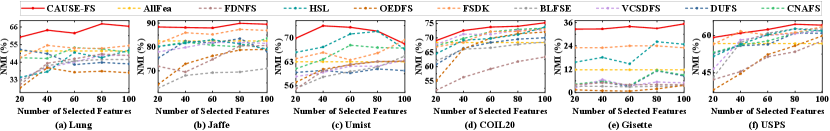
Performance Comparisons. Table II summarizes the performance of CAUSE-FS and other comparison methods in terms of ACC and NMI, with the best performance highlighted in boldface. As observed, CAUSE-FS consistently achieves the highest performance across all datasets and metrics when compared to other methods. As to Lung and Gisette datasets, CAUSE-FS achieves an average improvement of over 16% in ACC and 20% in NMI. As to Jaffe dataset, CAUSE-FS obtains an average improvement of over 12% in both ACC and NMI. As to Umist and USPS datasets, CAUSE-FS gains over 8% and 9% average improvement in terms of ACC and NMI, respectively. As to COIL20 dataset, CAUSE-FS achieves almost 6% average improvement in both ACC and NMI. Furthermore, to comprehensively assess the effectiveness of CAUSE-FS, we also present the results for all methods across varying numbers of selected features. Figs. 3 and 4 show the ACC and NMI values for all methods across different numbers of selected features. It is evident that CAUSE-FS outperforms other competing methods in most cases when the number of selected features ranges from 20 to 100. The superior performance of CAUSE-FS is attributed to two aspects: the joint learning of feature selection and confounder balancing, facilitating the identification of causally informative features, and the maintenance of a more reliable local structure by enhancing the importance of causal features in constructing the similarity graph.

Interpretability. To illustrate the interpretability of CAUSE-FS, we provide visualizations of the features selected by both CAUSE-FS and the runner-up method on COIL20, Jaffe, and USPS datasets. Due to limited space, we only present a few examples in Fig. 5. As shown in Fig. 5, CAUSE-FS selects features concentrated in the critical regions of objects, such as the body of a car, a person’s face, and the contours of a digit, whereas the runner-up methods tend to select numerous irrelevant contextual features. From the perspective of interpretability, CAUSE-FS can select causally informative features from unlabeled data to enhance downstream tasks like clustering. This ability enables it to explain why an image is assigned to the “car” cluster by identifying causal features, such as the car body.

Parameter Sensitivity and Convergence Analysis. The proposed method CAUSE-FS involves three tuning parameters, i.e., $\alpha$ , $\lambda$ and $\beta$ . To investigate the impact of parameters on CAUSE-FS, Fig. 6 shows the performance variations of CAUSE-FS as one parameter is varied while the others are kept fixed, across different numbers of selected features. We can observe that CAUSE-FS exhibits minor fluctuations when $\alpha$ is around 100, whereas it maintains relative stability w.r.t. $\beta$ and $\lambda$ . Furthermore, Fig. 7 displays the convergence curves of CAUSE-FS, showing that the proposed optimization algorithm quickly reduces the objective function value and converges within 20 iterations.

Ablation Study. We conduct an ablation study comparing CAUSE-FS with two of its variants to evaluate the contributions of its two key modules.

CAUSE-FS-I (without generalized causal regression module):

		$\displaystyle\min_{\bm{\Theta}}\frac{1}{2}\sum_{i,j=1}^{n}\sum_{m=1}^{M}\left[\\|\bm{X}_{\cdot i}^{T}\bm{R}^{(m)}\bm{W}-\bm{X}_{\cdot j}^{T}\bm{R}^{(m)}\bm{W}\\|_{2}^{2}\mathnormal{S}_{ij}^{(m)}\right.$		(17)
		$\displaystyle+\!\gamma_{m}\\|\bm{S}^{(m)}\!\\|_{\mathrm{F}}^{2}]\!-\!\!\operatorname{Tr}(\bm{G}^{\top}\!\!\sum_{m=1}^{M}\!\nu_{m}\bm{S}^{(m)})\!+\!\xi\\|\bm{G}\\|_{\mathrm{F}}^{2}\!+\!\lambda\\|\bm{W}\\|_{2,1}$		(17)

CAUSE-FS-II (without multi-granular adaptive graph learning module):

		$\displaystyle\min_{\bm{\Theta}}\!\sum_{i=1}^{n}\alpha\\|\mu_{i}\bm{X}_{\cdot i}^{\top}\bm{W}\!-\!\bm{F}_{i\cdot}\\|_{\mathrm{2}}^{2}+\operatorname{Tr}(\bm{F}^{\top}\bm{L}_{S}\bm{F})+\lambda\\|\bm{W}\\|_{2,1}$		(18)
		$\displaystyle+\beta\sum_{r=1}^{d}\\|\frac{1}{\|\Lambda_{t}\|}\sum_{i\in\Lambda_{t}}\phi(\mu_{i}Z_{\cdot i}^{r})-\frac{1}{\|\Lambda_{c}\|}\sum_{j\in\Lambda_{c}}\phi(\mu_{j}Z_{\cdot j}^{r})\\|_{\mathcal{H}_{\kappa}}^{2}$		(18)

The constraints in CAUSE-FS-I and CAUSE-FS-II are the same as those in Eq. (5).

Table III shows the results of the ablation experiments on six datasets. We observe that the performance of CAUSE-FS-I significantly decreases compared to CAUSE-FS regarding ACC and NMI. This highlights the effectiveness of the joint learning of feature selection and confounding balancing in identifying causally informative features. Moreover, CAUSE-FS consistently outperforms CAUSE-FS-II across all datasets, demonstrating that the multi-granular adaptive graph learning module can construct a more reliable similarity graph.

TABLE III: Average performance comparison of CAUSE-FS and its two variants in terms of ACC and NMI.

Datasets	CAUSE-FS		CAUSE-FS-I		CAUSE-FS-II
Datasets	ACC	NMI	ACC	NMI	ACC	NMI
Lung	79.98	59.64	44.99	24.98	75.50	57.53
Jaffe	84.11	88.35	59.49	61.90	79.04	82.26
Umist	55.29	69.86	35.57	46.38	53.34	66.07
COIL20	58.51	69.05	33.79	46.41	56.54	65.99
Gisette	81.09	32.62	57.38	2.86	75.31	20.60
USPS	65.91	59.20	39.46	26.44	60.84	50.86

7 Conclusion

In this paper, we have proposed a novel UFS method from the causal perspective, addressing the limitations of existing UFS methods that overlook the underlying causal mechanisms within data. The proposed CAUSE-FS framework integrates feature selection with confounding balance into a joint learning model, effectively mitigating spurious correlations between features and clustering labels, thereby facilitating the identification of causal features. Furthermore, CAUSE-FS enhances the reliability of local data structures by prioritizing the influence of causal features over non-causal features during the construction of the similarity graph. Extensive experiments conducted on six benchmark datasets demonstrate the superiority of CAUSE-FS over SOTA methods.

References

[1] K. Lagemann, C. Lagemann, B. Taschler, and S. Mukherjee, “Deep Learning of Causal Structures in High Dimensions under Data Limitations,” Nature Machine Intelligence, vol. 5, no. 11, pp. 1306–1316, 2023.
[2] M. T. Islam and L. Xing, “Deciphering the feature representation of deep neural networks for high-performance ai,” IEEE Transactions on Pattern Analysis and Machine Intelligence, vol. 46, no. 8, pp. 5273–5287, 2024.
[3] J. Li, K. Cheng, S. Wang, F. Morstatter, R. P. Trevino, J. Tang, and H. Liu, “Feature selection: A data perspective,” ACM Computing Surveys, vol. 50, no. 6, pp. 1–45, 2017.
[4] C. Hou, R. Fan, L. Zeng, and D. Hu, “Adaptive Feature Selection with Augmented Attributes,” IEEE Transactions on Pattern Analysis and Machine Intelligence, vol. 45, no. 8, pp. 9306–9324, 2023.
[5] S. Karami, F. Saberi-Movahed, P. Tiwari, P. Marttinen, and S. Vahdati, “Unsupervised feature selection based on variance–covariance subspace distance,” Neural Networks, vol. 166, pp. 188–203, 2023.
[6] G. Li, Z. Yu, K. Yang, M. Lin, and C. P. Chen, “Exploring feature selection with limited labels: A comprehensive survey of semi-supervised and unsupervised approaches,” IEEE Transactions on Knowledge and Data Engineering, vol. 1, no. 1, pp. 1–20, 2024.
[7] K. Yu, Y. Yang, and W. Ding, “Causal feature selection with missing data,” ACM Transactions on Knowledge Discovery from Data, vol. 16, no. 4, pp. 1–24, 2022.
[8] F. Quinzan, A. Soleymani, P. Jaillet, C. R. Rojas, and S. Bauer, “Drcfs: Doubly robust causal feature selection,” in International Conference on Machine Learning, 2023, pp. 28 468–28 491.
[9] F. Nie, Z. Ma, J. Wang, and X. Li, “Fast sparse discriminative k-means for unsupervised feature selection,” IEEE Transactions on Neural Networks and Learning Systems, vol. 35, no. 7, pp. 9943–9957, 2023.
[10] Y. Mi, H. Chen, C. Luo, S.-J. Horng, and T. Li, “Unsupervised feature selection with high-order similarity learning,” Knowledge-Based Systems, vol. 285, p. 111317, 2024.
[11] A. Yuan, M. You, D. He, and X. Li, “Convex non-negative matrix factorization with adaptive graph for unsupervised feature selection,” IEEE Transactions on Cybernetics, vol. 52, no. 6, pp. 5522–5534, 2020.
[12] H. Lim and D.-W. Kim, “Pairwise dependence-based unsupervised feature selection,” Pattern Recognition, vol. 111, p. 107663, 2021.
[13] P. Zhou, X. Wang, and L. Du, “Bi-level ensemble method for unsupervised feature selection,” Information Fusion, vol. 100, p. 101910, 2023.
[14] M. Mozafari, S. A. Seyedi, R. P. Mohammadiani, and F. A. Tab, “Unsupervised feature selection using orthogonal encoder-decoder factorization,” Information Sciences, vol. 663, p. 120277, 2024.
[15] R. Shang, L. Gao, H. Chi, J. Kong, W. Zhang, and S. Xu, “Non-convex feature selection based on feature correlation representation and dual manifold optimization,” Expert Systems with Applications, vol. 250, p. 123867, 2024.
[16] P. Cui, W. Hu, and J. Zhu, “Calibrated reliable regression using maximum mean discrepancy,” Advances in Neural Information Processing Systems, vol. 33, pp. 17 164–17 175, 2020.
[17] U. Maulik and S. Bandyopadhyay, “Performance evaluation of some clustering algorithms and validity indices,” IEEE Transactions on Pattern Analysis and Machine Intelligence, vol. 24, no. 12, pp. 1650–1654, 2002.
[18] X. Li, H. Zhang, R. Zhang, Y. Liu, and F. Nie, “Generalized uncorrelated regression with adaptive graph for unsupervised feature selection,” IEEE Transactions on Neural Networks and Learning Systems, vol. 30, no. 5, pp. 1587–1595, 2018.
[19] F. Nie, W. Zhu, and X. Li, “Unsupervised feature selection with structured graph optimization,” in Proceedings of the AAAI Conference on Artificial Intelligence, 2016, pp. 1302–1308.
[20] F. Nie, R. Zhang, and X. Li, “A generalized power iteration method for solving quadratic problem on the stiefel manifold,” Science China Information Sciences, vol. 60, pp. 1–10, 2017.
[21] A. Kumagai and T. Iwata, “Unsupervised domain adaptation by matching distributions based on the maximum mean discrepancy via unilateral transformations,” in Proceedings of the AAAI Conference on Artificial Intelligence, 2019, pp. 4106–4113.
[22] J. Benesty, J. Chen, Y. Huang, and I. Cohen, Eds., Pearson Correlation Coefficient. Berlin, Heidelberg: Springer Berlin Heidelberg, 2009.
[23] H. Wang, Y. Yang, and B. Liu, “Gmc: Graph-based multi-view clustering,” IEEE Transactions on Knowledge and Data Engineering, vol. 32, no. 6, pp. 1116–1129, 2019.
[24] F. Bach and M. Jordan, “Learning spectral clustering,” Advances in Neural Information Processing Systems, vol. 16, pp. 1–8, 2003.
[25] C. Hou, F. Nie, X. Li, D. Yi, and Y. Wu, “Joint embedding learning and sparse regression: A framework for unsupervised feature selection,” IEEE Transactions on Cybernetics, vol. 44, no. 6, pp. 793–804, 2013.
[26] X. Li, H. Zhang, R. Zhang, and F. Nie, “Discriminative and uncorrelated feature selection with constrained spectral analysis in unsupervised learning,” IEEE Transactions on Image Processing, vol. 29, pp. 2139–2149, 2019.
[27] H. Chen, F. Nie, R. Wang, and X. Li, “Fast unsupervised feature selection with bipartite graph and $\ell_{2,0}$ -norm constraint,” IEEE Transactions on Knowledge and Data Engineering, vol. 35, no. 5, pp. 4781–4793, 2022.