Causal Meta-Mediation Analysis: Inferring Dose-Response Function From Summary Statistics of Many Randomized Experiments
Abstract.
It is common in the internet industry to use offline-developed algorithms to power online products that contribute to the success of a business. Offline-developed algorithms are guided by offline evaluation metrics, which are often different from online business key performance indicators (KPIs). To maximize business KPIs, it is important to pick a north star among all available offline evaluation metrics. By noting that online products can be measured by online evaluation metrics, the online counterparts of offline evaluation metrics, we decompose the problem into two parts. As the offline A/B test literature works out the first part: counterfactual estimators of offline evaluation metrics that move the same way as their online counterparts, we focus on the second part: causal effects of online evaluation metrics on business KPIs. The north star of offline evaluation metrics should be the one whose online counterpart causes the most significant lift in the business KPI. We model the online evaluation metric as a mediator and formalize its causality with the business KPI as dose-response function (DRF). Our novel approach, causal meta-mediation analysis, leverages summary statistics of many existing randomized experiments to identify, estimate, and test the mediator DRF. It is easy to implement and to scale up, and has many advantages over the literature of mediation analysis and meta-analysis. We demonstrate its effectiveness by simulation and implementation on real data.
1. Introduction
Nowadays it is common in the internet industry to develop algorithms that power online products using historical data. The one that improves evaluation metrics from historical data will be tested against the one that has been in production to assess the lift in key performance indicators (KPIs) of the business in online A/B tests. Here we refer to metrics calculated from historical data as offline metrics and metrics calculated in online A/B tests as online metrics. In many cases, offline evaluation metrics are different from online business KPIs. For instance, a ranking algorithm, which powers search pages in e-commerce platforms, typically optimizes for relevance by predicting purchase or click probabilities of items. It could be tested offline (offline A/B tests) for rank-aware evaluation metrics, for example, normalized discounted cumulative gain (NDCG), mean reciprocal rank (MRR) or mean average precision (MAP), which are calculated from the test set of historical purchase or click-through feedback of users. Most e-commerce platforms, however, deem sitewide gross merchandise value (GMV) as their business KPI and test for it online. There could be various reasons not to directly optimize for business KPIs offline or use business KPIs as offline evaluation metrics, such as technical difficulty, business reputation, or user loyalty. Nonetheless, the discrepancy between offline evaluation metrics and online business KPIs poses a challenge to product owners because it is not clear that, in order to maximize online business KPIs, which offline evaluation metric should be adopted to guide the offline development of algorithms.
The challenge essentially asks for the causal effects of increasing offline evaluation metrics on business KPIs, e.g., how business KPIs would change for a 10% increase in an offline evaluation metric. The offline evaluation metric in which a 10% increase could result in the most significant lift in business KPIs should be the north star to guide algorithm development. Algorithms developed offline power online products, and online products contribute to the success of the business (see Figure 1). By noting that online products can be measured by online evaluation metrics, the online counterparts of offline evaluation metrics, we decompose the problem into two parts. The offline A/B test literature (see, e.g, Gilotte et al. (2018)) works out the first part (the black arrow): counterfactual estimators of offline evaluation metrics to bridge the inconsistency between changes of offline and online evaluation metrics. We focus on the second part (the red arrow): the causality between online products (assessed by online evaluation metrics) and the business (assessed by online business KPIs). The offline evaluation metric whose online counterpart causes the most significant lift in online business KPIs should be the north star. Hence, the question for us becomes, how business KPIs would change for a 10% increase in an online evaluation metric.
Randomized controlled trials, or online A/B tests, are popular to measure the causal effects of online product change on business KPIs. Unfortunately, they cannot answer our question directly. In online A/B tests, in order to compare the business KPIs caused by different values of an online evaluation metric, we need to fix the metric at its different values for treatment and control groups. Take the ranking algorithm as an example. If we could fix online NDCG of the search page at 0.22 and 0.2 for treatment and control groups respectively, then we would know how sitewide GMV would change for a 10% increase in online NDCG at 0.2. However, this experimental design is impossible, because most online evaluation metrics depend on users’ feedback and thus cannot be directly controlled.
We address the question by developing a novel approach of causal inference. We model the causality between online evaluation metrics and business KPIs by dose-response function (DRF) in potential outcome framework (Imbens, 2000; Imbens and Hirano, 2004). DRF originates from medicine and describes the magnitude of the response of an organism given different doses of a stimulus. Here we use it to depict the value of a business KPI given different values of an online evaluation metric. Different from doses of stimuli, values of online evaluation metrics cannot be directly manipulated. However, they could differ between treatment and control groups in experiments of treatments other than algorithms—user interface/user experience (UI/UX) design, marketing, etc. This could be due to the “fat hand” (Peysakhovich and Eckles, 2018; Yin and Hong, 2019) nature of online A/B tests that a single intervention can change many causal variables at once. A change of the tested feature, which is not algorithm, could induce users to change their engagement with algorithm-powered online products, so that values of online evaluation metrics would change. For instance, in an experiment of UI design, users might change their search behaviors because of the new UI design, so that values of online NDCG, which depends on search interaction, would change, even though ranking algorithm does not change. The evidence suggests that online evaluation metrics could be mediators that (partially) transmit causal effects of treatments on business KPIs in experiments where treatments are not necessarily algorithm-related. Hence, we formalize the problem as the identification, estimation, and test of mediator DRF.
In mediation analysis literature, there are two popular identification techniques: sequential ignorability (SI) and instrumental variable (IV). SI assumes each potential mediator is independent of all potential outcomes conditional on the assigned treatment, whereas IV permits dependence between unknown factors and mediators but forbids the existence of direct effects of the treatment. Rather than making these stringent assumptions, we leverage trial characteristics to explain average direct effect (ADE) in each experiment so that we can tease it out from average treatment effect (ATE) to identify the causal mediation. The utilization of trial characteristics means we have to use data from many trials because we need variations in trial characteristics. Hence, we develop our framework as a meta-analysis and propose an algorithm that only uses summarized results from many existing experiments and gain the advantage of easy implementation to scale.
Most meta-analyses rely on summarized results from different studies with different raw data sources. Therefore, it is almost impossible to learn more beyond the distribution of ATEs. Fortunately, the internet industry produces plentiful randomized trials with consistently defined metrics, and thus presents an opportunity for performing a more complicated meta-analysis. Literature is lacking in this area while we create the framework of causal meta-mediation analysis (CMMA) to fill in the gap.
Another prominent strength of our approach in real application is, for a new product that has been shipped online but has few A/B tests, it is plausible to explore the causality between its online metrics and business KPIs from many A/B tests of other products. The values of online metrics of the new product can differ between treatment and control groups in experiments of other products (”fat hand” (Peysakhovich and Eckles, 2018; Yin and Hong, 2019)), which makes it possible to solve for mediator DRF of the new product without its own A/B tests.
Note that, our approach can be applied to any evaluation metric that is defined at experimental-unit level, like metrics discussed in offline A/B test literature. The experimental unit means the unit for randomization in online A/B tests. For example, in search page experiments, the experimental unit is typically the user. Also, the evaluation metric can be any combination of existing experimental-unit-level metrics.
To summarize, our contributions in this paper include:
-
(1)
This is the first study that offers a framework to choose the north star among all available offline evaluation metrics for algorithm development to maximize business KPIs when offline evaluation metrics and business KPIs are different. We decompose the problem into two parts. Since the offline A/B test literature works out the first part: counterfactual estimators of offline evaluation metrics to bridge the inconsistency between changes of offline and online metrics, we work out the second part: inferring causal effects of online evaluation metrics on business KPIs. The offline evaluation metric whose online counterpart causes the most significant lift in business KPIs should be the north star. We show the implementation of our framework on data from Etsy.com.
-
(2)
Our novel approach CMMA combines mediation analysis and meta-analysis to identify, estimate, and test mediator DRF. It relaxes standard SI assumption and overcomes the limitation of IV, both of which are popular in causal mediation literature. It extends meta-analysis to solve causal mediation while the meta-analysis literature only learns the distribution of ATE. We demonstrate its effectiveness by simulation and show its performance is superior to other methods.
-
(3)
Our novel approach CMMA uses only trial-level summary statistics (i.e., meta-data) of many existing trials, which makes it easy to implement and to scale up. It can be applied to all experimental-unit-level evaluation metrics or any combination of them. Because it solves for causality problem of a product by leveraging trials of all products, it could be particularly useful in real applications for a new product that has been shipped online but has few A/B tests.
2. Literature Review
We draw on two strands of literature: mediation analysis and meta-analysis. We briefly discuss them in turn.
2.1. Mediation Analysis
Our framework expands on causal mediation analysis. Mediation analysis is actively conducted in various disciplines, such as psychology (MacKinnon et al., 2006; Rucker et al., 2011), political science (Green et al., 2010; Imai et al., 2010), economics (Heckman and Pinto, 2015), and computer science (Pearl, 2001). The recent application in the internet industry reveals the performance of recommendation system could be cannibalized by search in e-commerce website (Yin and Hong, 2019). Mediation analysis originates from the seminal paper of Baron and Kenny (1986), where they proposed a parametric estimator based on the linear structural equation model (LSEM). LSEM, by far, is still widely used by applied researchers because of its simplicity. Since then, Robins and Greenland (1992) and Pearl (2001) and other causal inference researchers have formalized the definition of causal mediation and pinpointed assumptions for its identification (Robins, 2003; Robins and Richardson, 2010; Pearl, 2014a) in various complicated scenarios. The progress features extensive usage of structural equation models and causal diagrams (e.g., NPSEM-IE of Pearl (2001) and FRCISTG of Robins (2003)).
As researchers extend the potential outcome framework of Rubin (2003) to causal mediation, alternative identification, and more general estimation strategies have been developed. Imai et al. (2010) achieved the non-parametric identification and estimation of mediation effects of a single mediator under the assumption of SI. After analyzing other well-known models such as LSEM (Baron and Kenny, 1986) and FRCISTG (Robins, 2003), they concluded that assumptions of most models can be either boiled down to or replaced by SI. However, SI is stringent, which ignites many in-depth discussions around it (see, e.g., the discussion between Pearl (2014a, b) and Imai et al. (2014)).
Another popular identification strategy of causal mediation is IV, which is a signature technique in economics (Angrist et al., 1996; Angrist and Krueger, 2001). Sobel (2008) used treatment as IV to identify mediation effects without SI. However, as Imai et al. (2010) pointed out, IV assumptions may be undesirable because they require all causal effects of the treatment pass through the mediator (i.e., complete mediation (Baron and Kenny, 1986)). Small (2012) proposed a new method to construct IV that allows direct effects of the treatment (i.e., partial mediation (Baron and Kenny, 1986)) but assumes that ADE of the treatment is the same for different segments of the population.
2.2. Meta-Analysis
Our method only uses summary statistics of many past experiments. Analyzing summarized results from many experiments is termed as meta-analysis and is common in analytical practice (Cooper et al., 2009; Stanley and Doucouliagos, 2012). In the literature, meta-analysis is used for mitigating the problem of external validity in a single experiment and learning knowledge that was hard to recover when analyzing data in isolation, such as heterogeneous treatment effects (see, e.g., Higgins and Thompson (2002); Browne and Jones (2017)). Besides, a significant advantage of meta-analysis is easy to scale, because it only takes summarized results from many different experiments.
Peysakhovich and Eckles (2018) took one step toward the direction of performing mediation analysis using data from many experiments. They used treatment assignments as IVs to identify causal mediation, which is similar to Sobel (2008), but lacks the justification why more than one experiment is needed and failed to address limitations of IV that we discussed above. Our framework shows that having access to many experiments enables identifying causal mediation without SI and overcoming the limitation of IV, both of which are hard to achieve with only one experiment.
3. Conceptual Framework
We follow the literature of potential outcomes (Rubin, 2003; Imai et al., 2010; Small, 2012) to set up our framework.
As illustrated in Figure 2, we suppose there are many experiments with different treatments, and there is a mediator that can be affected by any treatment and will in turn influence outcome . Each treatment may also affect directly. But we are particularly interested in recovering their shared casual channel, the link between and , marked in red in the figure. In the ranking algorithm example, is online evaluation metric of search page, is online business KPI. A challenge to identify the red link emerges if a confounder exists. could be (user engagement of) any other web-page/module or user preference in the ranking algorithm example. In the literature, there are two approaches to solve this challenge, SI and IV. SI requires that is observed and measured, and there are no other unmeasured/unobserved confounders after controlling for . The standard IV approach allows unmeasured/unobserved , but assumes no direct links between s and . An IV method proposed by Small (2012) relaxes requirements of standard approach, and assumes all s share a single direct link to . Our method allows unmeasured/unobserved and direct links from each to .
Suppose there are randomized trials in total. For each trial, there exists one treatment group and one control group111Experiments with multiple treatment arms can be considered as multiple trials with one treatment group and one control group.. To simplify the discussion, here we assume experimental units are first randomly assigned to different trials, and then randomly assigned into the treatment or control group of that trial. However, our approach CMMA allows the same unit to participate in multiple trials. We will go back to this point in Section 5.1.
We consider the following model for potential outcomes.
Definition 0.
| (1) | ||||
| (2) |
where the (, , , ) are i.i.d random vectors, for all , and .
We use a one-hot vector to encode the trial assignment where indicates the assignment to trial , and a binary variable to encode treatment assignment, with if assigned to the treatment group. For experimental unit with trial assignment and treatment assignment , the random variable represents the potential mediator, and the random variable represents the potential outcome that would be observed if were to receive or exhibit level of the mediator through some hypothetical mechanism.
We are interested in mediator DRF, which represents the value of given different values () of for the same and . This effectively is the red arrow in the Figure 2 for individuals. Let be the mediator DRF for individual . Our goal is to estimate average mediator DRF: , with which we can compute the percentage change of for a 10% increase in ceteris paribus. The expectation here is taken over the population of and so are other expectations in this paper if not specified. Here we consider polynomial mediator DRF: , which can capture the nonlinearity of the causality. Estimating means to estimate for . Vectors and are in . Each element of the vector, or , represents direct effect of the treatment on mediator or outcome in trial , and is assumed not to depend on .
Vectors and are also in , representing trial fixed effects. Random variables and represent idiosyncratic individual characteristics in the values of potential mediator and potential outcome. Assume 222This assumption can always be satisfied by reparameterizing and .. Let be the support of the distribution of mediator, and be the set containing all possible trial assignments.
We only observe realized data . The observed mediator , and observed outcome .
The specification has two implications. First, it implies that being in a particular trial will not affect mediator DRF. If mediator DRF is not trial independent, then having many trials only adds noises rather than provides additional information, and thus defeats the purpose of conducting a meta-analysis.
Remark (Trial-Irrelevant Mediator DRF).
| (3) |
for all , and , where does not depend on .
Second, the specification implies that there are no interaction effects between treatment and mediator on the outcome. It means the individual direct effect in each trial is irrelevant of the value of mediator. It is common in the literature of causal mediation (see, e.g., NPSEM-IE of Pearl (2001) and FRCISTG of Robins (2003)).

When mediator is not independent of (which is the case here), it is not trivial to recover through observed data. Figure 3 illustrates the challenge using simulated data. The grey lines in Figure 3 are simulated individual mediator DRFs following Definition 1, which represents the true causality between s and s. The blue line is the average mediator DRF. After randomly assign individuals to a trial, we can compute their observed mediator values and outcome values when in the control group, which are depicted by black scattered points. The black line shows the result from fitting the observed points by a widely-used non-parametric machine learning algorithm, locally estimated scatterplot smoothing (LOESS). Although the black line fits the data almost perfectly, it significantly deviates from the true underlying causality: the average mediator DRF.
4. Identification
4.1. Random Assignment
We first formally define the assumption that trial assignment and treatment assignment are random.
Assumption 1 (Random Assignment).
| (5) | ||||
| (6) |
for , all and and it is also assumed that for , all and .
Equation 6 can be guaranteed by random assignment of treatments in online A/B tests. Equation 5 means that individual’s potential outcomes and potential mediators are independent of the trial assignment. In practice, users are randomly selected into A/B tests, thus this assumption is trivially satisfied 333This is true regardless of whether the same unit can participate in multiple trials..
4.2. Relaxed Sequential Ignorability
Assumption 2 (Relaxed Sequential Ignorability).
| (7) |
for all , all , .
With Definition 1 and assumption that is a polynomial function, this assumption is equivalent to
for all , . This assumption says that the effect of changing on the outcome of is independent of the idiosyncratic individual unobservable that affects . A similar assumption is proposed by Small (2012, (IV-A3)). It means that the underlying causality between online product and the business is invariant even we observe some users produce higher online metrics than others for unknown reasons (i.e., the idiosyncratic unobservable). It is weaker than the SI. Whenever SI is satisfied, this assumption is naturally satisfied.444If for all then naturally is also independent of given . But the inverse is not true. It is possible to break SI and still fulfill this assumption. For example, when the mediator DRF is the same for all individuals and potential outcomes only depends on unobserved confounders, SI could be violated, while this assumption is still satisfied.
4.3. Trial-level Conditional Independence
In order to allow the presence of many direct treatment effects, we put some structure on the direct treatment effects. Let represents a vector of trial characteristics for trial .
Assumption 3 (Trial-Level Conditional Independence).
We assume ’s are independently and identically distributed with
and for all .
This assumption allows correlation between individual direct treatment effects on outcome and on mediator in a trial, while assuming such correlation disappears once conditioned on the characteristics of the trial. In the example of ranking algorithm, we may believe that experiments that test new algorithms generally have high impacts on both online NDCG and GMV whereas experiments that test new UI designs generally have only modest impacts on both metrics. But, within the same type of experiments, how much a treatment affects online NDCG does not correlate with its effect on GMV. This assumption is unverifiable. However, it is weaker than standard IV assumption in the literature. If there were no direct effects (IV assumption), then this assumption is trivially satisfied.
We can stack vectors of trial characteristics of all the trials into a matrix . Assumption 3 implies
| (8) |
for all .
4.4. Relevance Condition
Assumption 4 (Relevance Condition).
| (9) |
This assumption means, for the same type of experiments, direct treatment effect on () varies between experiments. It implies that treatment in each trial is still helpful for predicting after conditioning on trial-level covariates. This assumption is similar to the standard rank condition of IV identification (see Wooldridge (2010, Chapter 5)). Because can be calculated easily by summary statistics, this assumption can be empirically verified. In practice, since we can decide which trials to be included into the analysis, we can make sure this assumption always holds.
4.5. Identification of Mediator DRF
To simplify the proof, let’s assume . The same proof works for the more general polynomial DRF. Based on Definition 1, random variables of observed mediator and observed outcome can be written as
| (10) | ||||
| (11) | ||||
| where | ||||
With all the specifications and assumptions, we are ready to present the important result about the identification.
Theorem 1.
The proof is in Appendix A. Since can be identified from 10, we can use in place of . The proof shows that under Assumption 1 - 4, the covariances between and all the covariates, , and in Equation 12 are zeros. Therefore, structural parameters can be identified (see, e.g., Wooldridge (2010, Chapter 4) for more details of coefficient identification in linear regression).
The estimator from 2SLS of Theorem 1 is equivalent to an IV-2SLS estimator (see, e.g., Wooldridge (2010, Chapter 5) for more details of IV-2SLS). To see it, let’s rewrite Equation 11 as
| (13) |
where . We could get the same estimator of as in Theorem 1 through applying IV-2SLS on Equation 13 and using as instruments for .
5. Estimation and Hypothesis Testing
5.1. Estimation
Theorem 1 implies that average mediator effect can be estimated by running two regressions with pooled data. Such estimation could be very costly when the sample size in each trial is huge so that pooling data from all trials becomes infeasible. We propose a simpler two-stage procedure: CMMA.
Step 1-4 of CMMA calculates ATEs for each trial. ATE on and could be done in the standard procedure of online A/B tests. Step 5 and 6 uses only trial-level summary statistics and covariates, making it very easy to implement. This estimator has the same identification strategy as in Theorem 1 and is equivalent to a weight-adjusted 2SLS estimator. The proof is in Appendix B.
Note that, CMMA allows the same unit to participate in multiple trials. We can always use regression/ANOVA with treatment interaction terms to estimate ATEs of each trial for units in multiple trials, and then implement Step 5 and 6 of CMMA on estimated ATEs to get .
The most challenging part of applying CMMA is finding valid trial-level characteristics to satisfy Assumption 3. A good should have explanatory power for treatment effects on outcome and mediator across trials. However, similar to finding a valid instrument, there is no systematic way to produce . Practitioners have to rely on available data and domain knowledge to argue for the validity of . In Section 6 Table 2, we simulate the consequences of violating Assumption 3. In Section 7.2 Figure 4, we discuss the choice of in our real data application. Future work is required on the sensitivity of CMMA to .
5.2. Hypothesis Testing
In general, the reported standard errors from the second stage regression is slightly different from theoretical values without access to residuals in the first stage. But this becomes less of an issue as sample size increases. Since the sample size is usually enormous in online A/B tests, we recommend using the reported standard errors in the second stage regression for convenience.
Although we have assumed that for discussion to this point, the same proof is still valid for polynomial DRF, . Let and , where . Then we can use in place of in the proof. For our algorithm, in addition to and , we also need to estimate ATE on the higher order terms of , . 555Note: We need , not the -th order of : . .
To decide the highest -th order term to include in the model of the second stage, we can use the common model selection tool: Wald test. The standard way is to run a regression with higher-order terms and then perform a series of tests to check whether coefficients of those terms are zeros. See Greene (2011, Chapter 5) for more technical discussions on Wald test.
6. Simulation
We conduct Monte Carlo simulations to study the finite sample performance of our estimator. The details of our simulation set-up are described in Appendix C. The R code is available in our GitHub repository: https://github.com/znwang25/cmma.
We use Limited Information Maximum Likelihood (LIML) estimator as a benchmark to evaluate our CMMA estimator. An LIML estimator that is specified according to the simulation setup should have the best performance theoretically. We include two common estimators in the literature of mediation analysis into the comparison: Sobel (2008) and LSEM (Baron and Kenny, 1986), which are derived under identification approaches discussed in Section 2. Sobel (2008) assumes complete mediation, and LSEM (Baron and Kenny, 1986) relies on SI assumption (Imai et al., 2010). Both assumptions are false under our setting. We also implement the Full Sample 2SLS estimator prescribed in Theorem 1, which should produce similar results to CMMA.
| % of Wald Tests Rejecting | CMMA Estimation | ||||
| : | Highest Order of | Estimated ’s of | |||
| 3% | 5% | 100% | 1 | 4.016 | |
| 3% | 100% | 100% | 2 | 4.019, 1.999 | |
| 100% | 100% | 100% | 3 | 4.022, -0.001, 5 | |
-
•
Note: The sample size per trial is 1000 and the number of trials is 100. is rejected if p-value .
We set the sample size per trial (), to 200, 500, and 1000 and perform 100 simulations for each setting. Table 1 reports average biases and 95% confidence interval coverage of the estimators. The performance of CMMA is quite good and largely comparable to LIML’s result. When the sample size per trial is small, our estimator is slightly biased but the bias is much smaller than those of Sobel and LSEM estimators. As increases, the bias of our estimator decreases to zero, whereas the biases of the Sobel and LSEM estimators remain roughly the same. As the sample size is usually enormous in A/B tests (on average, one trial has millions of observations in the real data we obtained from an internet company), the bias of CMMA will be negligible in practice. Table 1 also shows that, as increases, the 95% confidence interval coverage of our estimator converges to the nominal coverage. This means that the OLS variance estimated in the trial-level regression is valid for hypothesis testing when is sufficiently large. In addition, the point estimate of Full Sample 2SLS estimator is numerically equal to CMMA, which empirically validates the equivalence claim made in Section 5.1.
In Table 2, we examine the performance of CMMA when each assumption fails. The results show that, the failure of Assumption 2 does not seem to affect the estimator’s unbiasedness, whereas with failures of Assumption 3 or 4, CMMA is no longer unbiased. Comparing results across rows, it seems to suggest that violating Assumption 4 has worse consequence in terms of bias. Fortunately, Assumption 4 is testable as discussed in Section 4.
We also test the performance of the Wald test with a higher order of . Table 3 shows that Wald tests can successfully select the correct model. For example, in the second row of Table 3, the true mediator DRF is a quadratic function of : . Wald tests in all simulations reject the null hypothesis that coefficients for the second-degree term and the third-degree term are zeros, whereas 97% of simulations fail to reject the hypothesis that coefficient for the third-degree term is zero. The result suggests that the highest order of should be 2. The last column of Table 4 shows that, with a correctly specified model, we can accurately estimate all the underlying parameters.
7. Application
We apply the approach on three most popular rank-aware evaluation metrics: NDCG, MRR, and MAP, to show, for ranking algorithms that power search page of Etsy.com, which one could lead to the most significant lift of sitewide GMV. Since the offline A/B test literature (Gilotte et al., 2018) bridges the inconsistency between changes of offline and online evaluation metrics, we only focus on, how sitewide GMV would change for 10% lifts in online NDCG, MRR, and MAP of search page respectively. All metrics in the application, unless otherwise noted, are online metrics. Please note the approach has not been deployed in Etsy. This work is not intended to apply to, nor is it a prediction of, actual live performance metrics or performance changes on Etsy or any other property.
7.1. User-Level Evaluation Metrics
We follow the offline A/B test literature (Gilotte et al., 2018) and define the three online rank-aware evaluation metrics at the user level. Although the three metrics are originally defined at the query level in the test collection evaluation of information retrieval (IR) literature, the search page in the industry is an online product for users and thus the computation could be adapted to the user level. More specifically, the three metrics are constructed as follows: 1) query-level metrics are computed using rank positions on search page and user conversion status as binary relevance, and non-conversion associated queries have zero values666If the user purchases the item that she has clicked on the search page, the relevance is 1; otherwise 0.; 2) user-level metrics is the average of query-level metrics across all queries the user issues (including non-conversion associated queries), and users who do not search or convert have zero values. Also, all the three metrics are defined at rank position 48, the lowest position of the first page of search results in Etsy.com.
7.2. Data
We have access to summarized results of 190 randomly selected experiments from the online A/B test platform of Etsy.com. All the experiments in the data have the user as an experimental unit. The data include descriptive information about each experiment such as the tested product change, the product team that initiated the experiment, and summary statistics of each experiment such as average (user-level) NDCG per user in treatment and control groups. Note that, the difference between the average metric per user in treatment and control groups is ATE on the metric (Step 1 - 4 in Algorithm 1).
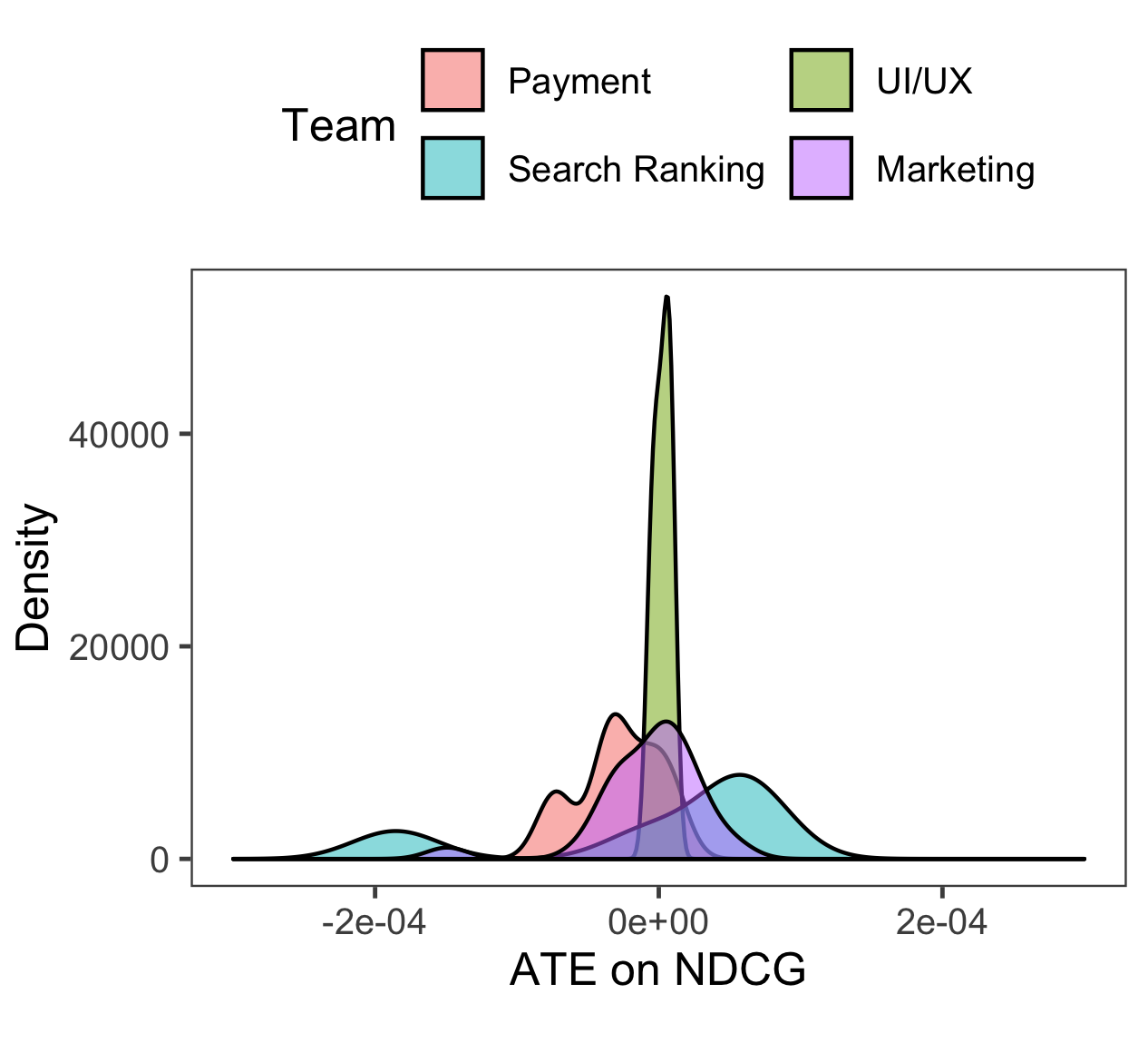
We use the taxonomy of product teams as our trial-level covariates because team taxonomy is quite informative of experiments as Figure 4 suggests. Figure 4 shows the density of ATE on NDCG for selected teams including UI/UX design, marketing, search ranking. First, it is evident that distributions of ATE on NDCG vary by team, which implies that Assumption 3 is likely to be satisfied. In particular, most experiments of the search ranking team post positive gains on NDCG, whereas experiments of the UI/UX team barely affects NDCG. Second, within each team there are significant variances of ATE on NDCG, which suggests that Assumption 4 holds. Due to page limitation, only results for NDCG are presented here, but the distributions of ATE on MAP and MRR exhibit the similar pattern.
7.3. Results
| P-Value | |||
| Null Hypothesis | : NDCG | : MAP | : MRR |
| 0.00119 | 0.02480 | 0.00346 | |
| 0.00018 | 0.00003 | 0.00000 | |
| 0.00018 | 0.00003 | 0.00000 | |
To decide the polynomial terms in the model, we perform Wald tests. The result from Wald tests is in Table 4. Since all the null hypothesis are rejected, the results suggest us including ATE on , ATE on and ATE on in the model of each (NDCG, MAP, MRR).

Figure 5 shows the estimation results. On the first row, blue lines depict estimated mediator DRFs. Scattered points represent summary statistics (the data for CMMA), ATE on ranking evaluation metrics and ATE on GMV, of all experiments. Black curves show results from fitting the data by LOESS. Note that, the range of three evaluation metrics could be much smaller than those in IR literature since they are defined at the user level (see Section 7.1). The estimated coefficients of mediator DRF are in Table D2 in the Appendix. The estimated mediator DRFs show that all three online metrics have positive causal effects on GMV. Note that, the causal relationships are different from the pattern of the data (scatter points and black curves). The differences between blue lines and black curves show the bias from fitting the data by machine learning methods without addressing omitted variables.
The second row of Figure 5 shows the elasticity of GMV: the percentage change of GMV for a 10% increase in each evaluation metric at its different values, which are derived from estimated mediator DRF. The downward slopes imply that, for all three evaluation metrics, as they increase, the benefit of continuous improving them on GMV decreases. For example, when average NDCG per user equals 0.0021, its 10% increase leads to a 9.88% increase in average GMV per user. Yet, when it equals 0.006, its 10% increase only leads to a 9.65% increase in average GMV per user.
Now it is easy for product owners to pick the evaluation metric that could guide algorithm development to achieve the most significant lift in online GMV. Suppose the current average values (per user) of NDCG, MAP, and MRR from live data are 0.00210, 0.00156, and 0.00153 respectively. From estimated mediator DRFs, we can calculate their corresponding elasticities of GMV: 9.88%, 9.87%, and 9.90%, which are marked by red lines in Figure 5. Because online MRR has the highest elasticity of GMV, we should choose offline MRR, which is estimated based on offline A/B test literature (Gilotte et al., 2018) and thus has the same move as online MRR, to guide the development of ranking algorithms.
8. Conclusion
In the internet industry, the algorithms developed offline power online products and online products contribute to the success of a business. In many cases, offline evaluation metrics, which guide algorithm development, are different from online business KPIs. It is important for product owners to pick the offline evaluation metric guided by which the algorithm could maximize online business KPIs. By noticing that online products could be assessed by online counterparts of offline evaluation metrics, we decompose the problem into two parts. Since the offline A/B test literature works out the first part: counterfactual estimators of offline evaluation metrics that move the same way as their online counterparts, we focus on the second part: inferring causal effects of online evaluation metrics on business KPIs. The offline evaluation metric whose online counterpart causes the most significant lift in online business KPIs should be the north star. We model online evaluation metrics as mediators and formalize the problem as to identify, estimate, and test mediator DRF. Our novel approach CMMA combines mediation analysis and meta-analysis and has many advantages over the two strands of literature. In particular, it takes as inputs only summary statistics from multiple past A/B tests, and thus it is easy to implement in scale. We apply the approach on Etsy’s real data to uncover the causality between three most popular rank-aware online evaluation metrics and GMV, and show how we successfully identify MRR as the offline evaluation metric for GMV maximization.
References
- (1)
- Angrist et al. (1996) Joshua Angrist, Guido Imbens, and Donald Rubin. 1996. Identification of Causal Effects Using Instrumental Variables. J. Amer. Statist. Assoc. 91, 434 (6 1996), 444.
- Angrist and Krueger (2001) Joshua Angrist and Alan Krueger. 2001. Instrumental Variables and the Search for Identification: From Supply and Demand to Natural Experiments. Journal of Economic Perspectives 15, 4 (11 2001), 69–85.
- Baron and Kenny (1986) Reuben Baron and David Kenny. 1986. The moderator-mediator variable distinction in social psychological research: Conceptual, strategic, and statistical considerations. Journal of Personality and Social Psychology 51, 6 (1986), 1173–1182.
- Browne and Jones (2017) Will Browne and Mike Jones. 2017. What works in e-commerce - a meta-analysis of 6700 online experiments. Qubit Digital Ltd (2017), 1–21.
- Cooper et al. (2009) Harris Cooper, Larry Hedges, and Jeffrey Valentine. 2009. The handbook of research synthesis and meta-analysis. Russell Sage Foundation.
- Gilotte et al. (2018) Alexandre Gilotte, Clément Calauzènes, Thomas Nedelec, Alexandre Abraham, and Simon Dollé. 2018. Offline A/B Testing for Recommender Systems. In Proceedings of the Eleventh ACM International Conference on Web Search and Data Mining (WSDM ’18). Association for Computing Machinery, New York, NY, USA, 198–206.
- Green et al. (2010) Donald Green, Shang Ha, and John Bullock. 2010. Enough already about ”Black Box” experiments: Studying mediation is more difficult than most scholars suppose. Annals of the American Academy of Political and Social Science 628, 1 (2010), 200–208.
- Greene (2011) William Greene. 2011. Econometric analysis (7 ed.). Pearson Education Inc. 1232 pages.
- Heckman and Pinto (2015) James Heckman and Rodrigo Pinto. 2015. Econometric Mediation Analyses: Identifying the Sources of Treatment Effects from Experimentally Estimated Production Technologies with Unmeasured and Mismeasured Inputs. Econometric Reviews 34 (2015), 6–31.
- Higgins and Thompson (2002) Julian Higgins and Simon Thompson. 2002. Quantifying heterogeneity in a meta-analysis. Statistics in Medicine 21, 11 (6 2002), 1539–1558.
- Imai et al. (2014) Kosuke Imai, Luke Keele, Dustin Tingley, and Teppei Yamamoto. 2014. Comment on Pearl: Practical implications of theoretical results for causal mediation analysis. Psychological Methods 19, 4 (2014), 482–487.
- Imai et al. (2010) Kosuke Imai, Luke Keele, and Teppei Yamamoto. 2010. Identification, Inference and Sensitivity Analysis for Causal Mediation Effects. Statist. Sci. (2010).
- Imbens (2000) Guido Imbens. 2000. The Role of the Propensity Score in Estimating Dose-Response Functions. Biometrika 87, 3 (2000), 706–710.
- Imbens and Hirano (2004) Guido Imbens and Keisuke Hirano. 2004. The Propensity Score with Continuous Treatments. (2004).
- MacKinnon et al. (2006) David MacKinnon, Amanda Fairchild, and Matthew Fritz. 2006. Mediation Analysis. Annual Review of Psychology 58, 1 (12 2006), 593–614.
- Pearl (2001) Judea Pearl. 2001. Direct and indirect effects. In Proceedings of the seventeenth conference on uncertainty in artificial intelligence. Morgan Kaufmann Publishers Inc., 411–420.
- Pearl (2014a) Judea Pearl. 2014a. Interpretation and identification of causal mediation. Psychological Methods 19, 4 (2014), 459–481.
- Pearl (2014b) Judea Pearl. 2014b. Reply to Commentary by Imai, Keele, Tingley, and Yamamoto Concerning Causal Mediation Analysis. Psychological Methods 19, 4 (2014), 488–492.
- Peysakhovich and Eckles (2018) Alexander Peysakhovich and Dean Eckles. 2018. Learning causal effects from many randomized experiments using regularized instrumental variables. In The Web Conference 2018 (WWW 2018). ACM, New York, NY.
- Robins (2003) James Robins. 2003. Semantics of causal DAG models and the identification of direct and indirect effects. Highly Structured Stochastic Systems (1 2003), 70–82.
- Robins and Greenland (1992) James Robins and Sander Greenland. 1992. Identifiability and exchangeability for direct and indirect effects. Epidemiology 3, 2 (1992), 143–155.
- Robins and Richardson (2010) James Robins and Thomas Richardson. 2010. Alternative graphical causal models and the identification of direct effects. Causality and psychopathology: finding the determinants of disorders and their cures (2010).
- Rubin (2003) Donald Rubin. 2003. Basic concepts of statistical inference for causal effects in experiments and observational studies. (2003).
- Rucker et al. (2011) Derek Rucker, Kristopher Preacher, Zakary Tormala, and Richard Petty. 2011. Mediation Analysis in Social Psychology: Current Practices and New Recommendations. Social and Personality Psychology Compass 5, 6 (2011), 359–371.
- Small (2012) Dylan Small. 2012. Mediation analysis without sequential ignorability: Using baseline covariates interacted with random assignment as instrumental variables. Journal of Statistical Research 46, 2 (2012), 91–103.
- Sobel (2008) Michael Sobel. 2008. Identification of Causal Parameters in Randomized Studies With Mediating Variables. Journal of Educational and Behavioral Statistics 33, 2 (2008), 230–251.
- Stanley and Doucouliagos (2012) Tom Stanley and Hristos Doucouliagos. 2012. Meta-regression analysis in economics and business. Routledge.
- Wooldridge (2010) Jeffrey Wooldridge. 2010. Econometric analysis of cross section and panel data. MIT Press, Cambridge, MA. 1096 pages.
- Yin and Hong (2019) Xuan Yin and Liangjie Hong. 2019. The Identification and Estimation of Direct and Indirect Effects in A/B Tests Through Causal Mediation Analysis. In Proceedings of the 25th ACM SIGKDD International Conference on Knowledge Discovery & Data Mining (KDD ’19). ACM, New York, NY, USA, 2989–2999.
Appendix A Proof of Theorem 1
Proof.
Let , and
, so Equation 12 can be written as
Because of assumption 4, is guaranteed to have full rank, thus is invertible. If we are able to show that , then can be estimated by linear projection . While this is infeasible, we can first estimate with its estimate and use in place of . Let be N-component data vector with ith element . The resulted estimator is the two-stage least squares(2SLS) estimator,
to estimate .
Note that, because of Assumption 1, 2 and 3, the following equations are true.
With the first component in ,
where the forth equality expands the matrix multiplication and the sixth equality follows from Assumption 3.
With respect to the third component,
where both the second and third equality follow from Assumption 1.
Taken together, we have shown that , therefore can be estimated by
∎
Appendix B Equivalence of CMMA and weight-adjusted 2SLS estimator
Let be an N-component data vector with ith element , be an N-component data vector with ith element , and , . The following proposition shows the link between CMMA and 2SLS estimator.
Proposition 0.
The CMMA method defined in Algorithm 1 is equivalent to a weight-adjusted 2SLS IV estimator with weight , where
Proof.
Let , . Since we are not particularly interested in coefficients in front of , using Frisch–Waugh–Lovell theorem, we can get 2SLS estimator for ,
We could use a weighting matrix and still get a consistent estimator for ,
.
Use
is equivalent to regressing on and and take coefficients of . And it is equivalent to regress on for each trial. ∎
Appendix C Simulation Setup
We follow the specification described in Equation 10 and Equation 12 and let the and be jointly normally distributed:
with . We fix the number of trials to be 50, and used independent uniform distributions to specify parameter value for each element of , . To satisfy Assumption 3 and 4, is set to be the sum of a dependent term and a random vector drawing from a uniform distribution. All the other parameter values are listed in the Table C1. The innovations in the error terms such as , elements of , and are all drawn from independent normal distributions .
| Parameters | Value |
| 4 | |
| , | |
| , | |
| , and = |
The one-hot group assignment variable and treatment indicator are randomly generated. We assume the 50 trials can be grouped into 3 experiment types and use experiment types as trial level covariates. Trials are randomly assigned into three types and is a matrix representing such assignment. Under this setup, all the assumptions are satisfied, and thus we are ready to estimate .
Appendix D Tables
| Dependent variable: GMS | |||
| : NDCG | : MPP | : MRR | |
| (1) | (2) | (3) | |
| 3,369.9∗ | 2,113.3 | 3,227.6 | |
| (1,753.3) | (2,600.2) | (2,368.2) | |
| 18,593.8∗∗∗ | 17,254.4∗ | 21,411.1∗∗ | |
| (6,606.5) | (9,718.6) | (8,882.6) | |
| 16,733.0∗∗∗ | 16,191.1∗∗ | 19,229.7∗∗∗ | |
| (5,162.6) | (7,213.5) | (6,576.5) | |
| Observations | 190 | 169 | 190 |
| R2 | 0.240 | 0.271 | 0.282 |
| Note: | ∗p0.1; ∗∗p0.05; ∗∗∗p0.01 | ||