11email: [email protected]
22institutetext: Microsoft Research, Beijing, China
22email: [email protected]
Causal Inference for Influence Propagation — Identifiability of the Independent Cascade Model
Abstract
Independent cascade (IC) model is a widely used influence propagation model for social networks. In this paper, we incorporate the concept and techniques from causal inference to study the identifiability of parameters from observational data in extended IC model with unobserved confounding factors, which models more realistic propagation scenarios but is rarely studied in influence propagation modeling before. We provide the conditions for the identifiability or unidentifiability of parameters for several special structures including the Markovian IC model, semi-Markovian IC model, and IC model with a global unobserved variable. Parameter identifiability is important for other tasks such as influence maximization under the diffusion networks with unobserved confounding factors.
Keywords:
influence propagation independent cascade model identifiability causal inference.1 Introduction
Extensive research has been conducted studying the information and influence propagation behavior in social networks, with numerous propagation models and optimization algorithms proposed (cf. [15, 2]). Social influence among individuals in a social network is intrinsically a causal behavior — one’s action or behavior causes the change of the behavior of his or her friends in the network. Therefore, it is helpful to view influence propagation as a causal phenomenon and apply the tools in causal inference to this domain.
In causal inference, one key consideration is the confounding factors caused by unobserved variables that affect the observed behaviors of individuals in the network. For example, we may observe that user A adopts a new product and a while later her friend B adopts the same new product. This situation could be because A influences B and causes B’s adoption, but it could also be caused by an unobserved factor (e.g. an unknown information source) that affects both A and B. Confounding factors are important in understanding the propagation behavior in networks, but so far the vast majority of influence propagation research does not consider confounders in network propagation modeling. In this paper, we intend to fill this gap by explicitly including unobserved confounders into the model, and we borrow the research methodology from causal inference to carry out our research.
Causal inference research has developed many tools and methodologies to deal with such unobserved confounders, and one important problem in causal inference is to study the identifiability of the causal model, that is, if we can identify the certain effect of an intervention, or identify causal model parameters, from the observational data. In this paper, we introduce the concept of identifiability in causal inference research to influence propagation research and study whether the propagation models can be identified from observational data when there are unobserved factors in the causal propagation model. We propose the extend the classical independent cascade (IC) model to include unobserved causal factors, and consider the parameter identifiability problem for several common causal graph structures. Our main results are as follows. First, for the Markovian IC model, in which each unobserved variable may affect only one observed node in the network, we show that it is fully identifiable. Second, for the semi-Markovian IC model, in which each unobserved variable may affect exactly two observed nodes in the network, we show that as long as a local graph structure exists in the network, then the model is not parameter identifiable. For the special case of a chain graph where all observed nodes form a chain and every unobserved variable affect two neighbors on the chain, the above result implies that we need to know at least parameters to make the rest parameters identifiable, where is the number of observed nodes in the chain. We then show a positive result that when we know parameters on the chain, the rest parameters are identifiable. Third, for the global hidden factor model where we have an unobserved variable that affects all observed nodes in the graph, we provide reasonable sufficient conditions so that the parameters are identifiable.
Overall, we view that our work starts a new direction to integrate rich research results from network propagation modeling and causal inference so that we could view influence propagation from the lens of causal inference, and obtain more realistic modeling and algorithmic results in this area. For example, from the causal inference lens, the classical influence maximization problem [15] of finding a set of nodes to maximize the total influence spread is really a causal intervention problem of forcing an intervention on nodes for their adoptions, and trying to maximize the causal effect of this intervention. Our study could give a new way of studying influence maximization that works under more realistic network scenarios encompassing unobserved confounders.
2 Related Work
Influence Propagation Modeling. As described in [2], the main two models used to describe influence propagation are the independent cascade model and the linear threshold model. Past researches on influence propagation mostly focused on influence maximization problems, such as [15, 22]. In these articles, they select seed nodes online, observe the propagation in the network, and optimize the number of activated nodes after propagation by selecting optimal seed nodes. Also, some works are studying the seed-node set minimization problem, such as [11]. However, in our work, we mainly consider restoring the parameters in the independent cascade model by observing the network propagation. After obtaining the parameters in the network, we can then base on this to accomplish downstream tasks including influence maximization and seed-node set minimization.
Causal Inference and Identifiability. For general semi-Markovian Bayesian causal graphs, [13] and [21] have given two different algorithms to determine whether a do effect is identifiable, and these two algorithms have both soundness and correctness. [14] also proves that the ID algorithm and the repeating use of the do calculus are equivalent, so for semi-Markovian Bayesian causal graphs, the do calculus can be used to compute all identifiable do effects.
In addition, for a special type of causal model, the linear causal model, articles [4] and [8] have given some necessary conditions and sufficient conditions on whether the parameters in the graph are identifiable with respect to the structure of the causal graph. However, the necessary and sufficient condition for parameter identifiability problem is not addressed and it remains an open question. In this paper, we study another special causal model derived from the IC model. Since the IC model can be viewed as a Bayesian causal model when the graph structure is a directed acyclic graph and it has some special properties, we try to give some necessary conditions and sufficient conditions for the parameters to be identifiable under some special graph structures.
3 Model and Problem Definitions
Following the convention in causal inference literature (e.g. [19]), we use capital letters () to represent variables or a set of variables, and their corresponding lower-case letters to represent their values. For a directed graph, we use ’s and ’s to represent nodes since each node will also be treated as a random variable in causal inference. For a node , we use and to represent the set of its out-neighbors and in-neighbors, respectively. When the graph is directed acyclic (DAG), we refer to a node’s in-neighbors as its parents and denote the set as . When we refer to the actual values of the parent nodes of , we use . For a positive integer , we use to denote . We use boldface letters to represent vectors, such as .
The classical independent cascade model [15] of influence diffusion in a social network is modeled as follows. The social network is modeled as a directed graph , where is the set of nodes representing individuals in the social network, and is the set of directed edges representing the influence relationship between the individuals. Each edge is associated with an influence probability (we assume that if ). Each node is either in state or state , representing the idle state and the active state, respectively. At time step , a seed set of nodes is selected and activated (i.e. their states are set to ), and all other nodes are in state . The propagation proceeds in discrete time steps . Let denote the set of nodes that are active by time , and let . At any time , the newly activated node tries to activate each of its inactive outgoing neighbors , and the activation is successful with probability . If successful, is activated at time and thus . The activation trial of on its out-neighbor is independent of all other activation trials. Once activated, nodes stay as active, that is, . The propagation process ends at a step when there are no new nodes activated. It easy to see that the propagation ends in at most steps, so we use to denote the final set of active nodes after the propagation.
Influence propagation is naturally a result of causal effect — one node’s activation causes the activation of its outgoing neighbors. If the graph is directed and acyclic, then the IC model on this graph can be equated to a Bayesian causal model. In fact, we can consider each node in the IC model as a variable, and for a node , it takes the value determined by . Obviously, this is equivalent to our definition in the IC model. IC model is introduced in [15] to model influence propagation in social networks, but in general, it can model the causal effects among binary random variables. In this paper, we mainly consider the directed acyclic graph (DAG) setting, which is in line with the causal graph setting in the causal inference literature [19]. We will discuss the extension to general cyclic graphs or networks in the appendix.
All variables are observable, and we call them observed variables. They correspond to observed behaviors of individuals in the social network. There are also potentially many unobserved (or hidden) variables that affecting individuals’ behaviors. We use to represent the set of unobserved variables. In the IC model, we assume each is a binary random variable with probability to be and probability to be , and all unobserved variables are mutually independent. We allow unobserved variables ’s to have directed edges pointing to the observed variables ’s, but we do not consider directed edges among the unobserved variables in this paper. If has a directed edge pointing to , we usually use to represent the parameter on this edge. It has the same semantics as the ’s in the classical IC model: if , then with probability successfully influence by setting its state to , and with probability ’s state is not affected by , and this influence or activation effect is independent from all other activation attempts on other edges. Thus, overall, in a network with unobserved or hidden variables, we use to represent the corresponding causal graph, where is the set of unobserved variables, is the set of observed variables, and is the set of directed edges. We assume that is a DAG, and the state of every unobserved variable is sampled from with parameter , while the state of every observed variable is determined by the states of its parents and the parameters on the incoming edges of following the IC model semantics. In the DAG , we refer to an observable node as a root if it has no observable parents in the graph. Every root has at least one unobserved parent. We use vectors to represent parameter vectors associated with edges among observed variables, edges from unobserved to observed variables, and unobserved nodes, respectively. We refer to the model as the causal IC model. When the distinction is needed, we use capital letters to represent the parameter names, and lower boldface letters to represent the parameter values.
In this paper, we focus on the parameter identifiability problem following the causal inference literature. In the context of the IC model, the states of nodes are observable while the states of are unobservable. We define parameter identifiability as follows.
Definition 1 (Parameter Identifiability)
Given a graph , we say that a set of IC model parameters on is identifiable if after fixing the values of parameters outside and fixing the observed probability distributions for all and all , the values of parameters in are uniquely determined. We say that the graph is parameter identifiable if . Accordingly, the algorithmic problem of parameter identifiability is to derive the unique values of parameters in given graph , the values of parameters outside , and the observed probability distributions for all and all . Finally, if the algorithm only uses a polynomial number of observed probability values ’s and runs in polynomial time, where both polynomials are with respect to the graph size, we say that the parameters in are efficiently identifiable.
Note that when there are no unobserved variables (except the unique unobserved variables for each root of the graph), the problem is mainly to derive the parameters ’s from all observed ’s. In this case, the parameter identifiability problem bears similarity with the well-studied network inference problem [10, 16, 9, 7, 18, 1, 3, 6, 5, 17, 20, 12]. The network inference problem focuses on using observed cascade data to derive the network structure and propagation parameters, and it emphasizes on the sample complexity of inferring parameters. Hence, when there are no unobserved variables in the model, we could use the network inference methods to help to solve the parameter identifiability problem. However, in real social influence and network propagation, there are other hidden factors that affect the propagation and the resulting distribution. Such hidden factors are not addressed in the network inference literature. In contrast, our study in this paper is focusing on addressing these hidden factors in network inference, and thus we borrow the ideas from causal inference to study the identifiability problem under the IC model.
In this paper, we study three types of unobserved variables that could commonly occur in network influence propagation. They correspond to three types of IC models with unobserved variables, as summarized below.
Markovian IC Model. In the Markovian IC model, each observed variable is associated with a unique unobserved variable , and there is a directed edge from to . This models the scenario where each individual in the social network has some latent and unknown factor that affects its observed behavior. We use to denote the parameter on the edge . Note that the effect of on the activation of is determined by probability , and thus we treat for all , and focus on identifying parameters ’s. Thus the graph has parameters , and . Figure 2 shows an example of a Markovian IC model. If some , it means that the observed variable has no latent variable influencing it, and it only receives influence from other observed variables.


Semi-Markovian IC Model. The second type of unobserved variables is the hidden variables connected to exactly two observed variables in the graph. In particular, for every pair of nodes , we allow one unobserved variable that has two edges, one pointing to and the other pointing to . This models the scenario that two individuals in the social network has a common unobserved confounder that may affect the behavior of two individuals. We call this type of model semi-Markovian IC model, following the common terminology of the semi-Markovian model in the literature [19]. In this model, each has a parameter , and edges and have parameters and respectively. Therefore, the graph has parameters , , and .
Within this model, we will pay special attention to a special type of graphs where the observed variables form a chain, i.e. , and the unobserved variables always point to the two neighbors on the chain. In this case, we use to denote the unobserved variable associated with edge , and the parameters on the edges and are denoted as and , respectively. Figure 3 represents this chain model.

IC Model with A Global Unobserved Variable. The third type of hidden variables is a global unobserved variable that points to all observed variables in the network. This naturally models the global causal effect where some common factor affects all or most individuals in the network. For every edge , we use to represent its parameter.
Moreover, we can combine this model with the Markovian IC model, where we allow both unobserved variable for each individual and a global unobserved varoable . Figure 2 represents this model.
4 Parameter Identifiability of the Markovian IC Model
For the Markovian IC model in which every observed variable has its own unobserved variable, we can fully identify the model parameters in most cases, as given by the following theorem.
Theorem 4.1 (Identifiability of the Markovian IC Model)
For an arbitrary Markovian IC model with parameters and , all the parameters are efficiently identifiable, and for every , if , then all parameters for are efficiently identifiable.
Proof
The theorem essentially says that all parameters are identifiable under the Markovian IC model, except for the corner case where some . In this case, the observed variable is fully determined by its unobserved parent , so we cannot determine the influence from other observed parents of to . But the influence from the observed parents of to is not useful any way in this case, so the edges from the observed parents of to will not affect the causal inference in the graph and they can be removed.
5 Parameter Identifiability of the Semi-Markovian IC Model
Following the definition in the model section, we then consider the identifiability problem of the semi-Markovian models. We will demonstrate that in most cases, this model is not parameter identifiable. Actually, from [21] we know that the semi-Markovian Bayesian causal model is also not identifiable in general. Essentially, our conclusion is not related to their result. On the other side, we will show that with some parameters known in advance, the semi-Markovian IC chain model will be identifiable.
5.1 Condition on Unidentifiability of the Semi-Markovian IC Model
More specifically, the following theorem shows the unidentifiability of the semi-Markovian IC model with a special structure in it.
Theorem 5.1 (Unidentifiability of the Semi-Markovian IC Model)
Suppose in a general graph , we can find the following structure. There are three observable nodes such that and unobservable with . Suppose each of only has two edges associated to it, the three nodes can be written adjacently in a topological order of nodes in . Then we can deduce that the graph is not parameter identifiable.
Figure 4 is an example of the structure described in the above theorem.

Proof (Outline)
To prove that the parameters in the model with this structure are not identifiable, we give two different sets of parameters directly. We show that these two different sets of parameters produce the same distribution of nodes in , and thus the set of parameters is not identifiable by observing only the distribution of . The details of these two sets of parameters and the distributions they produce are included in Appendix 0.A. ∎
5.2 Identifiability of the Chain Model
We now consider the chain model as described in Section 3 and depicted in Figure 3. In this structure, we present a conclusion of identifiability under the assumption that the valuations of some parameters are our prior knowledge.
We divide the parameters of the graph into four vectors
| (3) | |||
| (4) |
For the chain model, our theorem below shows that once the parameters is known, or is known, the set consists of remaining parameters in the chain is efficiently identifiable.
Theorem 5.2 (Identifiability of the Semi-Markovian IC Chain Model)
Suppose that we have a semi-Markovian IC chain model with the graph and the IC parameters , , and , and suppose that all parameters are in the range . If the values of parameter is known, or is known, then the remaining parameters are efficiently identifiable.
Proof (Outline)
We use induction to prove this theorem. Under the assumption that is known and or is known, suppose , , and has been determined by us, and we prove that and can also be determined. In fact, by the distribution of the first nodes on the chain we can obtain three different equations, and after substituting our known parameters, the inductive transition can be completed. It is worthy noting that this inductive process can also be used to compute the unknown parameters efficiently.
The proof is lengthy because of the many corner cases considered and the need to discuss the cases and . The details of this proof are included in Appendix 0.B.
According to Theorem 5.2 we get that the semi-Markovian chain is parameter identifiable in the case that particular parameters are known. Simultaneously, by Theorem 5.1, we can show that if just less than parameters are known, then this semi-Markovian chain will not be parameter identifiable. Actually, if the chain model is parameter identifiable, utilizing Theorem 5.1, we know that for each , at least one of parameters between and should be known. Therefore, we let , we can deduce that at least should be known. Formally, we have the following collary of Theorem 5.1 and Theorem 5.2.
Corollary 1
For a semi-Markovian IC chain model, if no more than parameters are known in advance, the remaining parameters are unidentifiable; if it is allowed to know parameters in advance, we can choose or to be known, then the remaining parameters are identifiable.
6 Parameter Identifiability of Model with a Global Hidden Variable
Next, we consider the case where there is a global hidden variable in the causal IC model, defined as those in Section 3. If there is only one hidden variable in the whole model, we prove that the parameters in general in this model are identifiable; if there is not only , the model is also Markovian, that is, there are also hidden variables corresponding to , then the parameters in this model are identifiable if certain conditions are satisfied.
6.1 Observable IC Model with Only a Global Hidden Variable
Suppose the observed variables in the connected DAG graph are in a topological order and there is a global hidden variable such that there exists an edge from to the node for each observable variable . Suppose the activating probability of is and the activating probability from to is (naturally, and there are at least of nonzero ’s). Now we propose a theorem according to these settings.
Theorem 6.1 (Identifiability of the IC Model with a Global Hidden Variable)
For an arbitrary IC model with a global hidden variable with parameters , and such that and for , all the parameters in and are identifiable.
Proof (Outline)
We discuss this problem in two cases, the first one is the existence of two disconnected points in and . At this point we can use to solve out , and then use and to solve out .
After getting , by the quotients of probabilities of propagating results, we can get all the parameters.
Another case is that there is no as described above. At this point there must exist three points that are connected with each other and . We observe the probabilities of different possible propagating results of these three points with all other nodes are after the propagation. From these, we can solve out , and then solve out all parameters by the same method as in the first case.∎
6.2 Markovian IC Model with a Global Hidden Variable (Mixed Model)
Suppose the model is , where , . Here, are in a topological order. The parameters are , , and .
Theorem 6.2 (Identifiability of Markovian IC Model with a Global Hidden Variable (Mixed Model))
For an arbitrary Markovian IC Model with a Global Hidden Variable with parameters , , and , we suppose that all the parameters are not . If such that each pair in are disconnected and , then the parameters and are identifiable. Moreover, if can be adjacently continuous in some topological order, i.e. without loss of generality, all the parameters are identifiable.
Proof (Outline)
Assuming that there exist that satisfy the requirements of the theorem, then we can write expressions for the distribution of these three parameters when all other nodes with subscripts not greater than are equal to . In fact, we can see that with these expressions, we can solve for and .
Since we have and , we will be able to obtain all the parameters very easily by dividing these equations two by two. This proof has some trivial discussion to show that this computational method does not fail due to corner cases. ∎
Notice that the parameters in this model are identifiable when and only when a special three-node structure appears in it. Intuitively, this is because through this structure we can more easily obtain some information about the parameters, which does not contradict the intuition of Theorem 5.1.
7 Conclusion
In this paper, we study the parameter identifiability of the independent cascade model in influence propagation and show conditions on identifiability or unidentifiability for several classes of causal IC model structure. We believe that the incorporation of observed confounding factors and causal inference techniques is important in the next step of influence propagation research and identifiability of the IC model is our first step towards this goal. There are many open problems and directions in combining causal inference and propagation research. For example, seed selection and influence maximization correspond to the intervention (or do effect) in causal inference, and how to compute such intervention effect under the network with unobserved confounders and how to do influence maximization is a very interesting research question. In terms of identifiability, one can also investigate the identifiability of the intervention effect, or whether given some intervention effect one can identify more of such effects. One can also look into identifiability in the general cyclic IC models, for which we provide some initial discussions in Appendix 0.E, but more investigations are needed.
References
- [1] Abrahao, B., Chierichetti, F., Kleinberg, R., Panconesi, A.: Trace complexity of network inference. arXiv e-prints pp. arXiv–1308 (2013)
- [2] Chen, W., Lakshmanan, L.V., Castillo, C.: Information and Influence Propagation in Social Networks. Morgan & Claypool Publishers (2013)
- [3] Daneshmand, H., Gomez-Rodriguez, M., Song, L., Schölkopf, B.: Estimating diffusion network structures: Recovery conditions, sample complexity & soft-thresholding algorithm. In: ICML (2014)
- [4] Drton, M., Foygel, R., Sullivant, S.: Global identifiability of linear structural equation models. The Annals of Statistics 39(2), 865–886 (2011)
- [5] Du, N., Liang, Y., Balcan, M., Song, L.: Influence function learning in information diffusion networks. In: ICML 2014, Beijing, China, 21-26 June 2014 (2014)
- [6] Du, N., Song, L., Gomez-Rodriguez, M., Zha, H.: Scalable influence estimation in continuous-time diffusion networks. In: NIPS 2013, December 5-8, 2013, Lake Tahoe, Nevada, United States. pp. 3147–3155 (2013)
- [7] Du, N., Song, L., Smola, A.J., Yuan, M.: Learning networks of heterogeneous influence. In: NIPS 2012, December 3-6, 2012, Lake Tahoe, Nevada, United States. pp. 2789–2797 (2012)
- [8] Foygel, R., Draisma, J., Drton, M.: Half-trek criterion for generic identifiability of linear structural equation models. The Annals of Statistics pp. 1682–1713 (2012)
- [9] Gomez-Rodriguez, M., Balduzzi, D., Schölkopf, B.: Uncovering the temporal dynamics of diffusion networks. arXiv preprint arXiv:1105.0697 (2011)
- [10] Gomez-Rodriguez, M., Leskovec, J., Krause, A.: Inferring networks of diffusion and influence. In: KDD’2010 (2010)
- [11] Goyal, A., Bonchi, F., Lakshmanan, L.V., Venkatasubramanian, S.: On minimizing budget and time in influence propagation over social networks. Social network analysis and mining 3(2), 179–192 (2013)
- [12] He, X., Xu, K., Kempe, D., Liu, Y.: Learning influence functions from incomplete observations. arXiv e-prints pp. arXiv–1611 (2016)
- [13] Huang, Y., Valtorta, M.: Identifiability in causal bayesian networks: A sound and complete algorithm. In: AAAI. pp. 1149–1154 (2006)
- [14] Huang, Y., Valtorta, M.: Pearl’s calculus of intervention is complete. arXiv preprint arXiv:1206.6831 (2012)
- [15] Kempe, D., Kleinberg, J.M., Tardos, É.: Maximizing the spread of influence through a social network. In: KDD (2003)
- [16] Myers, S.A., Leskovec, J.: On the convexity of latent social network inference. arXiv e-prints pp. arXiv–1010 (2010)
- [17] Narasimhan, H., Parkes, D.C., Singer, Y.: Learnability of influence in networks. In: Proceedings of the 29th Annual Conference on Neural Information Processing Systems (2015)
- [18] Netrapalli, P., Sanghavi, S.: Finding the graph of epidemic cascades. arXiv preprint arXiv:1202.1779 (2012)
- [19] Pearl, J.: Causality. Cambridge University Press (2009), 2nd Edition
- [20] Pouget-Abadie, J., Horel, T.: Inferring graphs from cascades: A sparse recovery framework. arXiv e-prints pp. arXiv–1505 (2015)
- [21] Shpitser, I., Pearl, J.: Identification of joint interventional distributions in recursive semi-markovian causal models. In: Proceedings of the 21st National Conference on Artificial Intelligence, 2006. pp. 1219–1226 (2006)
- [22] Tang, Y., Shi, Y., Xiao, X.: Influence maximization in near-linear time: A martingale approach. In: Proceedings of the 2015 ACM SIGMOD international conference on management of data. pp. 1539–1554 (2015)
Appendix
Appendix 0.A Proof for Unidentifiability of the Semi-Markovian IC Model (Theorem 5.1)
See 5.1
Proof
To prove that the parameters are unidentifiable, we will construct two different sets of valuations of parameters such that two distributions of values taken by the nodes in are the same. In fact, we assume that the parent nodes of are and for . And, the parameters are set as shown in Figure 4.
One set of parameters is that all the parameters are set to . Another set of parameters is that all the parameters are set to be except and . The exceptions are set to be
| (5) | |||
| (6) |
where is an arbitrary number between and . Then we only need to prove that for an arbitrary distribution of the ancestors of except , the distributions of are the same for the two parameter settings. This is because if this condition is satisfied, then the children of will not be affected by the differences of the parameter valuations because the parameters determining them are the same (only the distribution of will change but each of them only has two children that are in ). In fact, we have
| (7) | |||
| (8) | |||
| (9) | |||
| (10) | |||
| (11) | |||
| (12) | |||
| (13) | |||
| (14) | |||
| (15) | |||
| (16) | |||
| (17) | |||
| (18) | |||
| (19) | |||
| (20) | |||
| (21) | |||
| (22) | |||
| (23) |
Notice that these equations are only related to and , so until now, we have proved that the two sets of parameters produce two same distributions for observed variables and therefore is parameter unidentifiable at this point.∎
Appendix 0.B Proof for the Chain Structure (Theorem 5.2)
See 5.2
Proof
In the analysis, we use the following notations. For observed nodes , we use to represent their collective states as a bit string. For a bit string of length , we write
| (24) | ||||
Note that is observable, but and are not observable.
We will use induction method to prove this result. More specifically, we want to prove the base step that and are known. Moreover, we will prove the induction step that if , , and are already known, we can compute and using distributions of observed variables.
Initially, in order to complete the induction step, we divide the problem into two cases which are and .
Firstly, if , we only need to compute . Actually, we have the following relations of and other known variables. If , we have
| (25) | ||||
If and , we have
| (26) | ||||
If and , we have
| (27) | ||||
We should notice that are both determined by the parameters we already know, hence, we can see the three types of recursions as functions of and . We only need to prove that we can solve the three parameters from these functions. In order to simplify the equations, we define some notations as below where .
| (28) | ||||
It is easy to verify that . According to these, we have
| (29) |
which is equivalent to
| (30) | ||||
To show the relation of the coefficients of and , we prove two lemmas at first.
Lemma 1
For two arbitrary string with the same lengths, we prove that the equation is impossible.
Proof
Actually, if , we have . We can verify that
| (31) | ||||
which is impossible if all the terms are not zero.∎
Lemma 2
As we defined above, we have the following equation if the denominators are not zero:
| (32) |
Proof
Actually, we can compute the left hand side of Equation 32 as below:
| (33) | ||||
So the lemma is proved. We should also notice that this lemma holds not only for , it is true for because and are defined the same as Equation 28.∎
Now we prove that Equation 25 and Equation 30 are two linear independent equations for unknown variables and . We only need to prove that the ratio of coefficients of and are different in these two equations. Because otherwise, we have
| (34) |
which is impossible because . Until now, we have proved that when is equal to , we can compute if the other parameters are already known.
Now we consider the case that , and we need to prove that if , we can use , , and to compute and . First, we propose a lemma to illustrate the recurrence relationship of the distributions.
Lemma 3
Suppose is a string with items, then we have the following relations:
| (35) |
| (36) |
| (37) |
| (38) |
Moreover, we have the following relations of and other known variables. If , we have
| (39) |
If and , we have
| (40) | ||||
If and , we have
| (41) | ||||
Each of these equations is only one more factor compared to the case, so we can still get the similar result
| (42) | ||||
which is an equation of and . Since we assume that or is known, we can get both and by this equation. Then we can get by Equation 39 using . Then all the terms in Equation 40 except are known and not , so we can get . This completes the inductive transition.
Finally, we consider the base case. We only need to prove that if is known, one of and is known, then and the unknown one between can be computed using and . Actually, we have the following equations
| (43) | |||
| (44) | |||
| (45) |
When we know and , we can get the other parameters as below
| (46) | |||
| (47) | |||
| (48) | |||
| (49) | |||
| (50) |
When we know and , we can get the other parameters as below
| (51) | |||
| (52) | |||
| (53) | |||
| (54) | |||
| (55) |
Notice that all the denominators in these solutions are not , therefore, we have proved the base case. Until now, we have proved the whole theorem.∎
Appendix 0.C Proof for the Model with a Global Hidden Variable (Theorem 6.1)
See 6.1
Proof
We have the following equations
| (56) | ||||
such that is not a child of . Therefore, for each pair of unconnected nodes, if two of them () satisfy , we can get . Then we can use the following two equations to solve :
| (57) | ||||
If we see and as two unknown variables, they can be solved by this system of linear equations. With the value of , we can solve out by using for . For , it can be computed by if . We suppose the parents of are such that . Therefore, we have
| (58) | ||||
if . Hence, we can still get all the meaningful . Until now, we have got all the parameters solved.
Now we consider the case that such that and . This is equivalent to the claim that for all the such that , they form a complete graph if we remove all the directions of edges. Suppose three of them are . Then we can get the following equations:
| (59) | ||||
Therefore, can all be solved. Then we can use the same procedure to get all the and then all the parameters.
In conclusion, we have solved the identifiability problem of the model with a global hidden variable.∎
Appendix 0.D Proof for the Mixed Model (Theorem 6.2)
See 6.2
Proof
In order to simplify our proof, we introduce some new notations. Suppose we already have as required in description of this theorem.
| (60) | ||||
| (61) | ||||
| (62) | ||||
Therefore, we can easily verify that . Moreover, because are disconnected with each other, we have the following equations.
| (63) | ||||
Here, are known because are observable. Therefore, we can solve out using the equations. The result is shown as below.
| (64) | ||||
We can verify that
| (65) | |||
| (66) |
Therefore, there is only one solution of which is positive because
| (67) | |||
| (68) | |||
| (69) | |||
| (70) | |||
| (71) | |||
| (72) |
Because is fixed now, we can get according to . This process can be done if and only if the denominator is not zero, which is equivalent to . Therefore, we only need to find satisfying the conditions in the theorem and .
Notice that is an arbitrary number not less than , we can get and can be computed using and . For parameter , we can compute it using
| (73) | |||
| (74) | |||
| (75) | |||
| (76) |
Then we can get and and their division is what we want. Until now, we have proved the first part of the theorem. Now suppose we have . Then for an arbitrary string with bits, we still have the following facts.
| (77) | ||||
where or . Therefore, we can still have that equations the same as Equation 63 and from those equations, we can solve out all of the probabilities in the facts above. Using those probabilities, we can directly get all the parameters with indexes not larger than . Together with the conclusion of the first part of this theorem, all the parameters are determined.∎
Appendix 0.E Discussion on the Cyclic Models
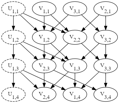
In the last section in appendix, we will introduce how to transform a general IC model to a causal model so that we can use do calculus method to identify do effects. In fact, since the propagation of the IC model takes place for at most rounds [2], we formulate that the state of in round is and that has three values, and , for three states. We construct a causal graph from these nodes with subscripts of time. Here, state means that the node is not activated, means that the node was activated at the last time point, and state means that the node is activated and has already tried to activate its child nodes. Moreover, all edges are defined as and . Furthermore, we define the following propagating equations.
| (78) | |||
| (79) | |||
| (80) | |||
| (81) | |||
| (82) | |||
| (83) | |||
| (84) |
By definition, we obtain that as a Bayesian causal model, so we can use the do calculus method [19] to solve out the identifiable do effects. For example, suppose has as observed nodes and as an unobserved node. The edges in are and . There exists a cycle in so it cannot be seen as a DAG. However, utilizing our transformation, the result graph is in Figure 5, which is a Bayesian causal model.