Catenoid limits of singly periodic minimal surfaces with Scherk-type ends

Hao Chen Institute of Mathematical Sciences, ShanghaiTech University, 201210 Pudong, Shanghai, China chenhao5@shanghaitech.edu.cn , Peter Connor Department of Mathematical Sciences, Indiana University South Bend pconnor@iusb.edu and Kevin Li School of Science, Engineering, and Technology, Penn State Harrisburg khl3@psu.edu

Abstract.

We construct families of embedded, singly periodic minimal surfaces of any genus $g$ in the quotient with any even number $2n>2$ of almost parallel Scherk ends. A surface in such a family looks like $n$ parallel planes connected by $n-1+g$ small catenoid necks. In the limit, the family converges to an $n$ -sheeted vertical plane with $n-1+g$ singular points termed nodes in the quotient. For the nodes to open up into catenoid necks, their locations must satisfy a set of balance equations whose solutions are given by the roots of Stieltjes polynomials.

Key words and phrases:

minimal surfaces, saddle towers, node opening

2010 Mathematics Subject Classification:

Primary 53A10

H. Chen was partially supported by Individual Research Grant from Deutsche Forschungsgemeinschaft within the project “Defects in Triply Periodic Minimal Surfaces”, Projektnummer 398759432.

The goal of this paper is to construct families of singly periodic minimal surfaces (SPMSs) of any genus in the quotient with any even number $2n>2$ of Scherk ends (asymptotic to vertical planes). Each family is parameterized by a small positive real number $\tau>0$ . In the limit $\tau\to 0$ , the Scherk ends tend to be parallel, and the surface converges to an $n$ -sheeted vertical plane with singular points termed nodes. As $\tau$ increases, the nodes open up into catenoid necks, and the surface looks like parallel planes connected by these catenoid necks.

There are many previously known examples of such SPMSs. Scherk [Sch35] discovered the examples with genus zero and four Scherk ends, in 1835. Karcher [Kar88] generalized Scherk’s surface in 1988 with any even number $2n>2$ of Scherk ends. In this paper, examples of genus 0 will be called “Karcher–Scherk saddle towers” or simply “saddle towers”, and saddle towers with four Scherk ends will be called “Scherk saddle towers”. Karcher also added handles between adjacent pairs of ends, producing SPMSs of genus $n$ with $2n$ Scherk ends. Traizet glued Scherk saddle towers into SPMSs of genus $(n^{2}-3n+2)/2$ with $2n>2$ Scherk ends because he was desingularizing simple arrangements of $n>1$ vertical planes. In 2006, Martín and Ramos Batista [MRB06] replaced the ends of Costa surface by Scherk ends, thereby constructed an embedded SPMS of genus one with six Scherk ends and, for the first time, without any horizontal symmetry plane. Hauswirth, Morabito, and Rodríguez [HMR09] generalized this result in 2009, using an end-to-end gluing method to replace the ends of Costa–Hoffman–Meeks surfaces by Scherk ends, thereby constructed SPMSs of higher genus with six Scherk ends. In 2010, da Silva and Ramos Batista [dSRB10] constructed a SPMS of genus two with eight Scherk ends based on Costa surface. Also, Hancco, Lobos, and Ramos Batista [HLB14] constructed SPMSs with genus $2n$ and $2n$ Scherk ends in 2014.

The examples of da Silva and Ramos Batista as well as all examples of Traizet admit catenoid limits that can be constructed using techniques in the present paper.

One motivation of this work is an ongoing project that addresses to various technical details in the gluing constructions.

Roughly speaking, given any “graph” $G$ that embeds in the plane and minimizes the length functional, one could desingularize $G\times\mathbb{R}$ into a SPMS by placing a saddle tower at each vertex. Previously, this was only proved for simple graphs under the assumption of an horizontal reflection plane [Tra96, Tra01]. Recently, we managed to allow the graph to have parallel edges, to remove the horizontal reflection plane by Dehn twist [CT21], and to prove embeddedness by analysing the bendings of Scherk ends [Che21].

However, we still require that the vertices of $G$ are neither “degenerate” nor “special”. Here, a vertex of degree $2k$ is said to be degenerate (resp. special) if $k$ (resp. $k-1$ ) of its adjacent edges extend in the same direction while other $k$ (resp. $k-1$ ) edges extend in the opposite direction. This limitation is due to the fact that a saddle tower with $2k$ Scherk ends can not have $k-1$ ends extending in the same direction while other $k-1$ ends extending in the opposite direction. Therefore, it is not possible to place a saddle tower at a degenerate or special vertex.

Nevertheless, we do know SPMSs that desingularize $G\times\mathbb{R}$ where $G$ is a graph with degenerate vertex. To include these in the gluing construction, we need to place catenoid limits of saddle towers, as those constructed in this paper, at degenerate vertices. From this point of view, the present paper can be seen as preparatory: The insight gained here will help us to glue saddle towers with catenoid limits of saddle towers in a future project.

This paper reproduces the main result of the thesis of the third named author [Li12]. Technically, the construction implemented in [Li12] was in the spirit of [Tra02b], which defines the Gauss map and the Riemann surface at the same time, and the period of the surface was assumed horizontal. Here, for the convenience of future applications, we present a construction in the spirit of [Tra08, CT21, Che21], which defines all three Weierstrass integrands by prescribing their periods, and the period of the surface is assumed vertical. In particular, we will reveal that a balance condition in [Li12] is actually a disguise of the balance of Scherk ends: The unit vectors in the directions of the ends sum up to zero.

Acknowledgements

We would like to thank the referee for many helpful comments.

1. Main result

1.1. Configuration

We consider $L+1$ vertical planes, $L\geq 1$ , labeled by integers $l\in[1,L+1]$ . Up to horizontal rotations, we assume that these planes are all parallel to the $xz$ -plane, which we identify to the complex plane $\mathbb{C}$ , with the $x$ -axis (resp. $z$ -axis) corresponding to the real (resp. imaginary) axis. We use the term “layer” for the space between two adjacent parallel planes. So there are $L$ layers.

We want $n_{l}\geq 1$ catenoid necks on layer $l$ , i.e. between the planes $l$ and $l+1$ , $1\leq l\leq L$ . For convenience, we adopt the convention that $n_{l}=0$ if $l<1$ or $l>L$ , and write $N=\sum n_{l}$ for the total number of necks. Each neck is labeled by a pair $(l,k)$ , where $1\leq l\leq L$ and $1\leq k\leq n_{l}$ .

To each neck is associated a complex number $q_{l,k}\in\mathbb{C}^{\times}=\mathbb{C}\setminus\{0\}$ , $1\leq l\leq L$ , $1\leq k\leq n_{l}$ . Then the positions of the necks are prescribed at $\ln q_{l,k}+2m\pi{\rm i}$ , $m\in\mathbb{Z}$ . Recall that the $z$ -axis is identified to the imaginary axis of the complex plane $\mathbb{C}$ , so the necks are periodic with period vector $(0,0,2\pi)$ . Note that, if we multiply $q_{l,k}$ ’s by the same complex factor $c$ , then the necks are all translated by $\ln c\pmod{2\pi{\rm i}}$ . So we may quotient out translations by fixing $q_{1,1}=1$ .

Moreover, each plane has two ends asymptotic to vertical planes. We label the end of plane $l$ that expands in the $-x$ (resp. $x$ ) direction by $0_{l}$ (resp. $\infty_{l}$ ). To be compatible with the language of graph theory that were used for gluing saddle towers [CT21], we use

\mathsf{H}=\{\eta_{l}\colon 1\leq l\leq L+1,\eta\in\{0,\infty\}\}

to denote the set of ends. When $0_{l}$ is used as subscript for parameter $x$ , we write $x_{l,0}$ instead of $x_{0_{l}}$ to ease the notation; the same applies to $\infty_{l}$ .

To each end is associated a real number $\dot{\theta}_{h}$ , $h\in\mathsf{H}$ . They prescribe infinitesimal changes of the directions of the ends. More precisely, for small $\tau$ , we want the unit vector in the direction of the end $h$ to have a $y$ -component or the order $\tau\dot{\theta}_{h}+\mathcal{O}(\tau^{2})$ .

Remark 1.

Multiplying $\dot{\theta}$ by a common real constant leads to a reparameterization of the family. Adding a common real constant to $\dot{\theta}_{l,0}$ and subtracting the same constant from $\dot{\theta}_{l,\infty}$ leads to horizontal rotations of the surface.

In the following, we write

q=(q_{l,k})_{\begin{subarray}{c}1\leqslant l\leqslant L\\ 1\leqslant k\leqslant n_{l}\end{subarray}}\quad\text{and}\quad\dot{\theta}=(\dot{\theta}_{h})_{h\in\mathsf{H}}.

Then a configuration refers to the pair $(q,\dot{\theta})$ .

1.2. Force

Given a configuration $(q,\dot{\theta})$ , let $c_{l}$ be the real numbers that solve

(1)

-n_{l}c_{l}+n_{l-1}c_{l-1}+\dot{\theta}_{l,0}+\dot{\theta}_{l,\infty}=0,\quad 1\leq l\leq L+1.

Recall the convention $n_{l}=0$ if $l<1$ or $l>L$ , so we also adopt the convention $c_{l}=0$ if $l<1$ or $l>L$ . A summation over $l$ yields

(2)

\Theta_{1}=\sum_{h\in\mathsf{H}}\dot{\theta}_{h}=0.

If (2) is satisfied, the real numbers $c_{l}$ are determined by (1) as functions of $\dot{\theta}$ .

For $1\leq l\leq L+1$ , let $\psi_{l}$ be the meromorphic $1$ -form on the Riemann sphere $\hat{\mathbb{C}}$ with simple poles at $q_{l,k}$ with residue $-c_{l}$ for each $1\leq k\leq n_{l}$ , at $q_{l-1,k}$ with residue $c_{l-1}$ for each $1\leq k\leq n_{l-1}$ , at $0$ with residue $\dot{\theta}_{l,0}$ , and at $\infty$ with residue $\dot{\theta}_{l,\infty}$ . More explicitly,

\psi_{l}=\Big{(}\sum_{k=1}^{n_{l}}\frac{-c_{l}}{z-q_{l,k}}+\sum_{k=1}^{n_{l-1}}\frac{c_{l-1}}{z-q_{l-1,k}}+\frac{\dot{\theta}_{l,0}}{z}\Big{)}dz.

We then see that Equations (1) arise from the Residue Theorem

Remark 2.

In the definition of configuration, we may replace $\dot{\theta}$ by the parameters $(c_{l},\dot{\theta}_{l+1,0}-\dot{\theta}_{l,0})_{1\leq l\leq L}$ . Then $\dot{\theta}_{l,0}$ ’s are defined up to an additive constant (corresponding to a rotation), $\dot{\theta}_{l,\infty}$ ’s are determined by (1), and (2) is automatically satisfied. To quotient out reparameterizations of the family, we may assume that $c_{l}=1$ for some $1\leq l\leq L$ .

We define the force $F_{l,k}$ by

(3)

F_{l,k}=\operatorname{Res}\left(\frac{\psi_{l}^{2}+\psi_{l+1}^{2}}{2}\frac{z}{dz},q_{l,k}\right).

Or, more explicitly,

(4)

F_{l,k}=\sum_{1\leq k\neq j\leq n_{l}}\frac{2c_{l}^{2}q_{l,k}}{q_{l,k}-q_{l,j}}-\sum_{1\leq j\leq n_{l+1}}\frac{c_{l}c_{l+1}q_{l,k}}{q_{l,k}-q_{l+1,j}}-\sum_{1\leq j\leq n_{l-1}}\frac{c_{l}c_{l-1}q_{l,k}}{q_{l,k}-q_{l-1,j}}\\ +c_{l}^{2}+c_{l}(\dot{\theta}_{l+1,0}-\dot{\theta}_{l,0}).

In [Li12], the force had different formula depending on the parity of $l$ . One verifies that both are equivalent to (4).

Remark 3 (Electrostatic interpretation).

The force equation (4) can be expressed as

F_{l,k}=\sum_{1\leq k\neq j\leq n_{l}}\frac{c_{l}^{2}(q_{l,k}+q_{l,j})}{q_{l,k}-q_{l,j}}-\sum_{1\leq j\leq n_{l+1}}\frac{c_{l}c_{l+1}(q_{l,k}+q_{l+1,j})}{2(q_{l,k}-q_{l+1,j})}\\ -\sum_{1\leq j\leq n_{l-1}}\frac{c_{l}c_{l-1}(q_{l,k}+q_{l-1,j})}{2(q_{l,k}-q_{l-1,j})}+\frac{c_{l}}{2}(\dot{\theta}_{l,\infty}-\dot{\theta}_{l,0}-\dot{\theta}_{l+1,\infty}+\dot{\theta}_{l+1,0}).

Note that

\frac{a+b}{a-b}=\coth\frac{\ln a-\ln b}{2}=\frac{2}{\ln a-\ln b}+\sum_{m=1}^{\infty}\Big{(}\frac{2}{\ln a-\ln b-2m\pi{\rm i}}+\frac{2}{\ln a-\ln b+2m\pi{\rm i}}\Big{)}.

Disregarding absolute convergence, we write this formally as

\frac{a+b}{a-b}=\sum_{m\in\mathbb{Z}}\frac{2}{\ln a-\ln b-2m\pi{\rm i}}.

Then the force is given, formally, by

F_{l,k}=\sum_{0\neq m\in\mathbb{Z}}\frac{2c_{l}^{2}}{2m\pi{\rm i}}+\sum_{\begin{subarray}{c}m\in\mathbb{Z}\\ 1\leq k\neq j\leq n_{l}\end{subarray}}\frac{2c_{l}^{2}}{\ln q_{l,k}-\ln q_{l,j}-2m\pi{\rm i}}\\ -\sum_{\begin{subarray}{c}m\in\mathbb{Z}\\ 1\leq j\leq n_{l+1}\end{subarray}}\frac{c_{l}c_{l+1}}{\ln q_{l,k}-\ln q_{l+1.j}-2m\pi{\rm i}}-\sum_{\begin{subarray}{c}m\in\mathbb{Z}\\ 1\leq j\leq n_{l-1}\end{subarray}}\frac{c_{l}c_{l-1}}{\ln q_{l,k}-\ln q_{l-1.j}-2m\pi{\rm i}}\\ +\frac{c_{l}}{2}(\dot{\theta}_{l,\infty}-\dot{\theta}_{l,0}-\dot{\theta}_{l+1,\infty}+\dot{\theta}_{l+1,0}).

Recall that $\ln q_{l,k}+2m\pi{\rm i}$ are the real positions of the necks. So this formal expression has an electrostatic interpretation similar to those in [Tra02b] and [Tra08]. Here, each neck interacts not only with all other necks in the same or adjacent layers, but also with background constant fields given by $\dot{\theta}$ .

Remark 4 (Another electrostatic interpretation).

In fact, $\eqref{eq:force}/q_{l,k}$ has a similar electrostatic interpretation. But this time, the necks are seen as placed at $q_{l,k}$ . Each neck interacts with all other necks in the same and adjacent layers, as well as a virtual neck at $0$ with “charge” $c_{l}+\dot{\theta}_{l+1,0}-\dot{\theta}_{l,0}$ . This is no surprise, as electrostatic laws are known to be preserved under conformal mappings (such as $\ln(z)$ ).

1.3. Main result

In the following, we write $F=(F_{l,k})_{1\leq l\leq L,1\leq k\leq n_{l}}$ .

Definition 1.

The configuration is balanced if $F=0$ and $\Theta_{1}=0$ .

Summing up all forces yields a necessary condition for the configuration to be balanced, namely

\Theta_{2}=\sum_{\begin{subarray}{c}1\leq l\leq L\\ 1\leq k\leq n_{l}\end{subarray}}F_{l,k}=\sum_{1\leq l\leq L+1}-\frac{1}{2}\Bigg{(}\operatorname{Res}\left(\frac{z\psi_{l}^{2}}{dz},0\right)+\operatorname{Res}\left(\frac{z\psi_{l}^{2}}{dz},\infty\right)\Bigg{)}\\ =\sum_{1\leq l\leq L+1}\frac{{\dot{\theta}_{l,\infty}^{2}-\dot{\theta}_{l,0}^{2}}}{2}=0.

Lemma 1.

The Jacobian matrix $\partial(\Theta_{1},\Theta_{2})/\partial\dot{\theta}$ has real rank $2$ as long as $c_{l}\neq 0$ for some $1\leq l\leq L$ .

The assumption of the lemma simply says that the surface does not remain a degenerate plane to the first order.

Proof.

The proposition says that the matrix has an invertible minor of size $2\times 2$ . Explicitly, we have

\frac{\partial(\Theta_{1},\Theta_{2})}{\partial(\dot{\theta}_{l,0},\dot{\theta}_{l,\infty})}=\begin{pmatrix}1&1\\ -\dot{\theta}_{l,0}&\dot{\theta}_{l,\infty}\end{pmatrix}.

This minor is invertible if and only if the ends $\dot{\theta}_{l,0}+\dot{\theta}_{l,\infty}\neq 0$ . This must be the case for at least one $1\leq l\leq L$ because, otherwise, we have $c_{l}=0$ for all $1\leq l\leq L$ . ∎

Definition 2.

The configuration is rigid if the complex rank of $\partial F/\partial q$ is $N-1$ .

Remark 5.

In fact, the complex rank of $\partial F/\partial q$ is at most $N-1$ . We have seen that a complex scaling of $q$ corresponds to a translation of $\ln q_{l,k}+2m\pi{\rm i}$ , $m\in\mathbb{Z}$ , which does not change the force. It then makes sense to normalize $q$ by fixing $q_{1,1}=1$ .

Theorem 1.

Let $(q,\dot{\theta})$ be a balanced and rigid configuration such that $c_{l}\neq 0$ for $1\leq l\leq L$ . Then for $\tau>0$ sufficiently small, there exists a smooth family $M_{\tau}$ of complete singly periodic minimal surface of genus $g=N-L$ , period $(0,0,2\pi)$ , and $2(L+1)$ Scherk ends such that, as $\tau\to 0$ ,

•

$M_{\tau}$ converges to an $(L+1)$ -sheeted $xz$ -plane with singular points at $\ln q_{l,k}+2m\pi{\rm i}$ , $m\in\mathbb{Z}$ . Here, the $xz$ -plane is identified to the complex plane $\mathbb{C}$ , with $x$ -axis (resp. $z$ -axis) identified to the real (resp. imaginary) axis.
•

After suitable scaling and translation, each singular point opens up into a neck that converges to a catenoid.
•

The unit vector in the direction of each Scherk end $h$ has the $y$ -component $\tau\dot{\theta}_{h}+\mathcal{O}(\tau^{2})$ .

Moreover, $M_{\tau}$ is embedded if

(5)

\dot{\theta}_{1,0}>\cdots>\dot{\theta}_{L+1,0}\quad\text{and}\quad\dot{\theta}_{1,\infty}>\cdots>\dot{\theta}_{L+1,\infty}.

Remark 6.

$M_{\tau}$ also depends smoothly on $\dot{\theta}$ belonging to the local smooth manifold defined by $\Theta_{1}=0$ and $\Theta_{2}=0$ . Up to reparameterizations of the family and horizontal rotations, we obtain families parameterized by $2L-1$ parameters. Since we have $2(L+1)$ Scherk ends, this parameter count is compatible with the fact that Karcher–Scherk saddle towers with $2k$ ends form a family parameterized by $2k-3$ parameters.

Remark 7.

If the embeddedness condition (5) is satisfied and $\Theta_{1}=0$ , the sequence $\dot{\theta}_{l,0}+\dot{\theta}_{l,\infty}$ is strictly monotonically decreasing, and changes sign once and only once. Then the sequence $n_{l}c_{l}$ is strictly concave (i.e. $n_{l-1}c_{l-1}+n_{l+1}c_{l+1}<2n_{l}c_{l}$ for $1\leq l\leq L$ ). Hence $c_{l}$ , $1\leq l\leq L$ , are strictly positive, and the condition of Lemma 1 is satisfied.

Remark 8.

We could allow some $c_{l}$ to be negative, with the price of losing embeddedness. Even worse, with negative $c_{l}$ , the vertical planes in the limit will not be geometrically ordered as they are labeled. For instance, if $L=2,c_{1}>0$ , but $c_{2}<0$ , then the catenoid necks, as well as the 1st and 3rd “planes”, will all lie on the same side of the 2nd “plane”.

Remark 9.

We did not allow any $c_{l}$ to be 0 in Theorem 1. Otherwise, the surface might still have nodes. In that case, the claimed family might not be smooth, and the claimed genus would be incorrect.

2. Examples

2.1. Surfaces of genus 0

When the genus $g=N-L=0$ , we have $n_{l}=1$ for all $1\leq l\leq L$ , i.e. there is only one neck on every layer. It then makes sense to drop the subscript $k$ . For instance, the position and the force for the neck on layer $l$ are simply denoted by $q_{l}$ and $F_{l}$ . We assume $L>1$ in this part.

In this case, if $\Theta_{1}=0$ , Equation (1) can be explicitly solved by

c_{l}=\sum_{i=1}^{l}(\dot{\theta}_{i,0}+\dot{\theta}_{i,\infty}),\quad 1\leq l\leq L,

and the force can be written in the form

F_{l}=-\widetilde{Q}_{l}+\widetilde{Q}_{l-1}+c_{l}(\dot{\theta}_{l,\infty}+\dot{\theta}_{l+1,0}),\quad 1\leq l\leq L,

where we changed to the parameters

\widetilde{Q}_{l}=\frac{c_{l+1}c_{l}}{1-q_{l+1}/q_{l}},\quad 1\leq l<L,

with the convention that $\widetilde{Q}_{0}=\widetilde{Q}_{L}=0$ . Then the forces are linear in $\widetilde{Q}$ and, if $\Theta_{2}=0$ , the balance condition $F=0$ is uniquely solved by

(6)

\widetilde{Q}_{l}=\sum_{i=1}^{l}c_{i}(\dot{\theta}_{i+1,0}+\dot{\theta}_{i,\infty})=-\sum_{i=l+1}^{L}c_{i}(\dot{\theta}_{i+1,0}+\dot{\theta}_{i,\infty}),\quad 1\leq l<L.

Therefore, if we fix $q_{1}=1$ , all other $q_{l}$ , $1<l\leq L$ are uniquely determined.

Recall from Remark 7 that, under the embeddedness condition (5), the numbers $c_{l}$ , $1\leq l\leq L$ , are positive. Moreover, the summands in (6) changes sign at most once, so the sequence $\widetilde{Q}$ is unimodal, i.e. there exists $1\leq l^{\prime}<L$ such that

0=\widetilde{Q}_{0}\leq\widetilde{Q}_{1}\leq\cdots\leq\widetilde{Q}_{l^{\prime}}\geq\cdots\geq\widetilde{Q}_{L-1}\geq\widetilde{Q}_{L}=0.

Hence $\widetilde{Q}_{l}$ , $1\leq l\leq L$ , are non-negative. Moreover,

	$\displaystyle\widetilde{Q}_{l}<\sum_{i=1}^{l}c_{i}(\dot{\theta}_{i,0}+\dot{\theta}_{i,\infty})$	$\displaystyle=\sum_{i=1}^{l}(c_{i}^{2}-c_{i-1}c_{i})\leq c_{l}^{2}\leq c_{l+1}c_{l}$	$\displaystyle\text{if }l<l^{\prime},$
	$\displaystyle\widetilde{Q}_{l}<-\sum_{i=l+1}^{L}c_{i}(\dot{\theta}_{i+1,0}+\dot{\theta}_{i+1,\infty})$	$\displaystyle=\sum_{i=l+1}^{L}(c_{i}^{2}-c_{i+1}c_{i})\leq c_{l+1}^{2}\leq c_{l+1}c_{l}$	$\displaystyle\text{if }l\geq l^{\prime}.$

So $q$ consists of real numbers and $q_{l+1}/q_{l}<0$ for all $1\leq l<L$ .

We have proved that

Proposition 2.

If the genus $g=N-L=0$ , and $\dot{\theta}$ satisfies the balancing condition $\Theta_{1}=\Theta_{2}=0$ as well as the embeddedness condition (5), then up to complex scalings, there exist unique values for the parameters $q$ , depending analytically on $\dot{\theta}$ , such that the configuration $(q,\dot{\theta})$ is balanced. Moreover, all such configurations are rigid. If we fix $q_{1}=1$ , then $q$ consist of real numbers, and we have $q_{l}>0$ (resp. $<0$ ) if $l$ is odd (resp. even).

2.2. Surfaces with four ends

When $L=1$ , $\Theta_{1}=\Theta_{2}=0$ implies that

\dot{\theta}_{1,0}+\dot{\theta}_{2,\infty}=\dot{\theta}_{2,0}+\dot{\theta}_{1,\infty}=0.

Up to reparameterizations of the family, we may assume that $c_{1}=1$ . It makes sense to drop the subscript $l$ in other notations, and write $F_{k}$ for $F_{1,k}$ , $q_{k}$ for $q_{1,k}$ , and $n$ for $n_{1}$ . The goal of this part is to prove the following classification result.

Proposition 3.

Up to a complex scaling, a configuration with $L=1$ and $n$ nodes must be given by $q_{k}=\exp(2\pi{\rm i}k/n)$ , and such a configuration is rigid.

Such a configuration is an $n$ -covering of the configuration for Scherk saddle towers. As a consequence, the arising minimal surfaces are $n$ -coverings of Scherk saddle towers. This is compatible with the result of [MW07] that the Scherk saddle towers are the only connected SPMSs with four Scherk ends.

Proof.

To find the positions $q_{k}$ such that

(7)

F_{k}=\sum_{1\leq k\neq j\leq n}\frac{2q_{k}}{q_{k}-q_{j}}-(n-1)=0,\qquad 1\leq k\leq n,

we use the polynomial method: Consider the polynomial

P(z)=\prod_{k=1}^{n}(z-q_{k}).

Then we have

	$\displaystyle P^{\prime}$	$\displaystyle=P\sum_{k=1}^{n}\frac{1}{z-q_{k}}$
	$\displaystyle P^{\prime\prime}$	$\displaystyle=P\sum_{k=1}^{n}\sum_{1\leq k\neq j\leq n}\frac{1}{z-q_{j}}\frac{1}{z-q_{k}}=2P\sum_{k=1}^{n}\frac{1}{z-q_{k}}\sum_{1\leq k\neq j\leq n}\frac{1}{q_{k}-q_{j}}$
		$\displaystyle=P\sum_{k=1}^{n}\frac{n-1}{q_{k}(z-q_{k})}=(n-1)P\sum_{k=1}^{n}\frac{1}{z}\Big{(}\frac{1}{q_{k}}+\frac{1}{z-q_{k}}\Big{)}\qquad\text{by~{}\eqref{eq:balance4ends}}$
		$\displaystyle=\frac{n-1}{z}\Big{(}P^{\prime}-\frac{P^{\prime}(0)}{P(0)}P\Big{)}$

For the last equation to have a polynomial solution, we must have $P^{\prime}(0)=0$ . Otherwise, the left-hand side would be a polynomial of degree $n-2$ , but the right-hand side would be a polynomial of degree $n-1$ .

Consequently, $F_{k}=0$ if and only if

zP^{\prime\prime}(z)-(n-1)P^{\prime}(z)=0,

which, up to a complex scaling, is uniquely solved by

P(z)=z^{n}-1.

So a balanced 4-end configuration must be given by the roots of unity $q_{k}=\exp(2\pi{\rm i}k/n)$ , $0\leq k\leq n-1$ .

We now verify that the configuration is rigid. For this purpose, we compute

\frac{\partial F_{k}}{\partial q_{j}}=\begin{dcases}2\frac{q_{k}}{(q_{k}-q_{j})^{2}},&j\neq k;\\ 2\sum_{1\leq k\neq i\leq n}\frac{-q_{i}}{(q_{k}-q_{i})^{2}},&j=k.\end{dcases}

Note that $\sum_{j=1}^{n}q_{j}\partial F_{k}/\partial q_{j}=0$ while

q_{j}\frac{\partial F_{k}}{\partial q_{j}}=2\frac{q_{j}q_{k}}{(q_{k}-q_{j})^{2}}=2\frac{e^{2\pi{\rm i}\frac{j+k}{n}}}{(e^{2\pi{\rm i}\frac{j}{n}}-e^{2\pi{\rm i}\frac{k}{n}})^{2}}\in\mathbb{R}_{<0}

when $j\neq k$ , so the matrix

\frac{\partial F}{\partial q}\operatorname{diag}(q_{1},\cdots,q_{n})

has real entries, has a kernel of complex dimension $1$ (spanned by the all-one vector), and any of its principal submatrix is diagonally dominant. We then conclude that the matrix, as well as the Jacobian $\partial F/\partial q$ , has a complex rank $n-1$ . This finishes the proof of rigidity. ∎

Remark 10.

The perturbation argument as in the proof of [Tra02b, Proposition 1] also applies here, word by word, to prove the rigidity.

2.3. Gluing two saddle towers of different periods

We want to construct a smooth family of configurations depending on a positive real number $\lambda$ such that, for small $\lambda$ , the configuration looks like two columns of nodes far away from each other, one with period $2\pi/n_{1}$ , and the other with period $2\pi/n_{2}$ . If balanced and rigid, these configurations would give rise to minimal surfaces that look like two Scherk saddle towers with different periods that are glued along a pair of ends. The construction is in the same spirit as [Tra02b, § 2.5] and [Tra08, § 4.3.4].

Proposition 4.

For a real number $\lambda>0$ sufficiently small, there are balanced and rigid configurations $(q(\lambda),\dot{\theta}(\lambda))$ with $L=2$ depending smoothly on $\lambda$ such that, at $\lambda=0$ ,

\frac{q_{2,j}}{q_{1,k}}=0,\qquad 1\leq k\leq n_{1},1\leq j\leq n_{2}.

Up to a complex scaling and reparameterization, we may fix $q_{1,1}=1$ , and write $q_{2,1}=\lambda\exp({\rm i}\phi)$ . Then, at $\lambda=0$ , we have

(8)

\dot{\theta}_{1,0}+\dot{\theta}_{2,\infty}=\dot{\theta}_{2,0}+\dot{\theta}_{3,\infty}=\dot{\theta}_{3,0}+\dot{\theta}_{1,\infty}=0

and,

	$\displaystyle q_{1,k}$	$\displaystyle=\exp\Big{(}\frac{k-1}{n_{1}}2\pi{\rm i}\Big{)},$	$\displaystyle 1\leq k\leq n_{1},$
	$\displaystyle\widetilde{q}_{2,k}:=q_{2,k}/q_{2,1}$	$\displaystyle=\exp\Big{(}\frac{k-1}{n_{2}}2\pi{\rm i}\Big{)},$	$\displaystyle 1\leq k\leq n_{2},$

where $\phi\operatorname{lcm}(n_{1},n_{2})$ is necessarily a multiple of $\pi$ .

In other words, the construction only works if the configuration admits a reflection symmetry.

Remark 11.

The first named author was shown a video suggesting that, when two Scherk saddle towers are glued into a minimal surface, one can slide one saddle tower with respect to the other while the surface remains minimal. The proposition above suggests that this is not possible.

In fact, the family of configurations also depends on $\dot{\theta}$ belonging to the local manifold defined by $\Theta_{1}=\Theta_{2}=0$ and (one equation from) (8). Up to rotations of the configuration and reparameterizations of the family of minimal surfaces, the family of configurations is parameterized, as expected, by two parameters.

Proof.

Let us first study the situation at $\lambda=0$ . We compute at $\lambda=0$

	$\displaystyle\frac{F_{1,k}}{c_{1}^{2}}=$	$\displaystyle\sum_{1\leq k\neq j\leq n_{1}}\frac{2q_{1,k}}{q_{1,k}-q_{1,j}}-\sum_{1\leq j\leq n_{2}}\frac{c_{2}}{c_{1}}\frac{q_{1,k}}{q_{1,k}-q_{2,j}}+1+\frac{\dot{\theta}_{2,0}-\dot{\theta}_{1,0}}{c_{1}}$
	$\displaystyle=$	$\displaystyle\sum_{1\leq k\neq j\leq n_{1}}\frac{2q_{1,k}}{q_{1,k}-q_{1,j}}-n_{2}\frac{c_{2}}{c_{1}}+1+\frac{\dot{\theta}_{2,0}-\dot{\theta}_{1,0}}{c_{1}},$
	$\displaystyle\frac{F_{2,k}}{c_{2}^{2}}=$	$\displaystyle\sum_{1\leq k\neq j\leq n_{2}}\frac{2q_{2,k}}{q_{2,k}-q_{2,j}}-\sum_{1\leq j\leq n_{1}}\frac{c_{1}}{c_{2}}\frac{q_{2,k}}{q_{2,k}-q_{1,j}}+1+\frac{\dot{\theta}_{3,0}-\dot{\theta}_{2,0}}{c_{2}}$
	$\displaystyle=$	$\displaystyle\sum_{1\leq k\neq j\leq n_{2}}\frac{2q_{2,k}}{q_{2,k}-q_{2,j}}+1+\frac{\dot{\theta}_{3,0}-\dot{\theta}_{2,0}}{c_{2}}.$

Write $G_{l}=\sum_{k}F_{l,k}$ . Summing the above over $k$ gives, at $\lambda=0$ ,

\frac{1}{n_{1}}\frac{G_{1}}{c_{1}^{2}}=n_{1}-n_{2}\frac{c_{2}}{c_{1}}+\frac{\dot{\theta}_{2,0}-\dot{\theta}_{1,0}}{c_{1}},\qquad\frac{1}{n_{2}}\frac{G_{2}}{c_{2}^{2}}=n_{2}+\frac{\dot{\theta}_{3,0}-\dot{\theta}_{2,0}}{c_{2}}.

So $G_{1}=G_{2}=0$ at $\lambda=0$ only if

	$\displaystyle 0=$	$\displaystyle-(\dot{\theta}_{2,0}+\dot{\theta}_{3,\infty})=\dot{\theta}_{3,0}-\dot{\theta}_{2,0}+n_{2}c_{2}$
	$\displaystyle=$	$\displaystyle-(\dot{\theta}_{1,0}+\dot{\theta}_{2,\infty})=n_{1}c_{1}-n_{2}c_{2}+\dot{\theta}_{2,0}-\dot{\theta}_{1,0}.$

This together with $\Theta_{1}=0$ proves (8).

Now assume that (8) is satisfied. Then we have, at $\lambda=0$

	$\displaystyle\frac{F_{1,k}}{c_{1}^{2}}=$	$\displaystyle\sum_{1\leq k\neq j\leq n_{1}}\frac{2q_{1,k}}{q_{1,k}-q_{1,j}}-(n_{1}-1),$
	$\displaystyle\frac{F_{2,k}}{c_{2}^{2}}=$	$\displaystyle\sum_{1\leq k\neq j\leq n_{2}}\frac{2q_{2,k}}{q_{2,k}-q_{2,j}}-(n_{2}-1).$

These expressions are identical to the force (7) for single layer configurations. So we know for $l=1,2$ that, at $\lambda=0$ , the configuration is balanced only if

\widetilde{q}_{l,k}:=\frac{q_{l,k}}{q_{l,1}}=\exp\Big{(}\frac{k-1}{n_{l}}2\pi{\rm i}\Big{)}.

Up to complex scaling, we may fix $q_{1,1}=1$ so $\widetilde{q}_{1,k}=q_{1,k}$ . And up to reparameterization of the family (of configurations), we write $q_{2,1}=\lambda\exp({\rm i}\phi)$ .

Now assume these initial values for $\widetilde{q}_{l,k}$ . Then we have, at $\lambda=0$ ,

	$\displaystyle\frac{G_{2}}{c_{1}c_{2}}=$	$\displaystyle-\sum_{k=1}^{n_{2}}\sum_{j=1}^{n_{1}}\frac{q_{2,k}}{q_{2,k}-q_{1,j}}=\sum_{k=1}^{n_{2}}\sum_{j=1}^{n_{1}}\sum_{m=1}^{\infty}\Big{(}\frac{q_{2,k}}{q_{1,j}}\Big{)}^{m}$
	$\displaystyle=$	$\displaystyle\sum_{k=1}^{n_{2}}\sum_{j=1}^{n_{1}}\sum_{m=1}^{\infty}q_{2,1}^{m}\exp\bigg{(}2m{\rm i}\pi\Big{(}\frac{k-1}{n_{2}}-\frac{j-1}{n_{1}}\Big{)}\bigg{)}$

Seen as a power series of $q_{2,1}$ , the coefficient for $q_{2,1}^{m}$ is

\sum_{k=1}^{n_{2}}\sum_{j=1}^{n_{1}}\exp\bigg{(}2m{\rm i}\pi\Big{(}\frac{k-1}{n_{2}}-\frac{j-1}{n_{1}}\Big{)}\bigg{)}.

It is non-zero only if $m$ is a common multiple of $n_{1}$ and $n_{2}$ , in which case the coefficient of $q_{2,1}^{m}$ equals $n_{1}n_{2}$ . In particular, let $\mu=\operatorname{lcm}(n_{1},n_{2})$ , then at $\lambda=0$ ,

(9)

\operatorname{Im}\frac{G_{2}}{\lambda^{\mu}}=c_{1}c_{2}n_{1}n_{2}\sin(\mu\phi)

vanishes if and only if $\mu\phi$ is a multiple of $\pi$ .

Now we use the Implicit Function Theorem to find balance configurations with $\lambda>0$ . From the proof for Proposition 3, we know that $\big{(}\frac{\partial F_{l,k}}{\partial\widetilde{q}_{l,j}}\big{)}_{2\leq j,k\leq n_{l}}$ , $l=1,2$ , are invertible. Hence for $\lambda$ sufficiently small, there exist unique values for $(\widetilde{q}_{l,k})_{l=1,2;2\leq k\leq n_{l}}$ , depending smoothly on $\lambda$ , $\dot{\theta}$ , and $\phi$ , such that $(F_{l,k})_{l=1,2;2\leq k\leq n_{l}}=0$ . By (9), there exists a unique value for $\phi$ , depending smoothly on $\lambda$ and $\dot{\theta}$ , such that $\operatorname{Im}G_{2}/\lambda^{\mu}=0$ . Note also that $\operatorname{Re}G_{2}$ is linear in $\dot{\theta}$ . By Lemma 1, the solutions $(\lambda,\dot{\theta})$ to $\operatorname{Re}G_{2}=0$ and $\Theta_{1}=\Theta_{2}=0$ form a manifold of dimension $4$ (including multiplication by common real factor on $\dot{\theta}$ and rotation of the configuration). Finally, we have $G_{1}=0$ by the Residue Theorem, and the balance is proved.

For the rigidity of the configurations with sufficiently small $\lambda$ , we need to prove that the matrix

\begin{pmatrix}\big{(}\frac{\partial F_{1,k}}{\partial q_{1,j}}\big{)}_{2\leq j,k\leq n_{1}}&&\\ &\big{(}\frac{\partial F_{2,k}}{\partial\widetilde{q}_{2,j}}\big{)}_{2\leq j,k\leq n_{2}}&\\ &&\frac{\partial G_{2}}{\partial q_{2,1}}\end{pmatrix}

is invertible. We know that the first two blocks are invertible at $\lambda=0$ . By continuity, they remain invertible for $\lambda$ sufficiently small. The last block is clearly non-zero for $\lambda\neq 0$ sufficiently small. ∎

2.4. Surfaces with six ends of type (n,1)

In this section, we investigate examples with $L=2$ (hence six ends), $n_{1}=n$ , $n_{2}=1$ . Up to a reparameterization of the family, we may assume that $c_{1}=1$ . Up to a complex scaling, we may assume that $q_{2,1}=1$ .

We will prove that $q_{1,k}$ ’s are given by the roots of hypergeometric polynomials. Let us first recall their definitions. A hypergeometric function is defined by

{{}_{2}F_{1}}(a,b;c;z)=\sum_{k=0}^{\infty}\frac{(a)_{k}(b)_{k}}{(c)_{k}}\frac{z^{k}}{k!}

with $a,b,c\in\mathbb{C}$ , $c$ is not a non-positive integer,

(a)_{k}=a(a+1)\cdots(a+k-1)=\frac{\Gamma(a+k)}{\Gamma(a)},

and $(a)_{0}=1$ . The hypergeometric function $w={{}_{2}F_{1}}(a,b;c;z)$ solves the hypergeometric differential equation

(10)

z(1-z)w^{\prime\prime}+[c-(a+b+1)z]w^{\prime}-abw=0.

If $a=-n$ is a negative integer,

{{}_{2}F_{1}}(-n,b;c;z):=\sum_{k=0}^{n}(-1)^{k}\binom{n}{k}\frac{(b)_{k}}{(c)_{k}}z^{k}

is a polynomial of degree $n$ , and is referred to as a hypergeometric polynomial.

Proposition 5.

Let $(q,\dot{\theta})$ be a balanced configuration with $L=2$ , $c_{1}=1$ , $n_{1}=n$ , $n_{2}=1$ . Then, up to a complex scaling, we have $q_{2,1}=1$ and $(q_{1,k})_{1\leq k\leq n}$ are the roots of the hypergeometric polynomial ${{}_{2}F_{1}}(-n,b;c;z)$ with

b:=n-c_{2}+\dot{\theta}_{2,0}-\dot{\theta}_{1,0},\qquad c:=1+\dot{\theta}_{2,0}-\dot{\theta}_{1,0}.

Moreover, as long as $b$ and $c$ are not non-positive integers, and $c-b$ is not a non-positive integer bigger than $-n$ , the configuration is rigid.

Proof.

The force equations are

\begin{split}F_{1,k}&=\sum_{1\leq k\neq j\leq n}\frac{2q_{1,k}}{q_{1,k}-q_{1,j}}-\frac{q_{1,k}c_{2}}{q_{1,k}-1}+c,1\leq k\leq n,\\ F_{2,1}&=-\sum_{j=1}^{n}\frac{c_{2}}{1-q_{1,j}}+c_{2}^{2}+c_{2}(\dot{\theta}_{3,0}-\dot{\theta}_{2,0}),\end{split}

where $c:=1+\dot{\theta}_{2,0}-\dot{\theta}_{1,0}$ . To solve $F_{1,k}=0$ for $k=1,2,\ldots,n$ , we use again the polynomial method: Let $P(z)=\prod_{k=1}^{n}(z-q_{1,k})$ . Then we have

	$\displaystyle P^{\prime}$	$\displaystyle=P\sum_{k=1}^{n}\frac{1}{z-q_{1,k}};$
	$\displaystyle P^{\prime\prime}$	$\displaystyle=2P\sum_{k=1}^{n}\frac{1}{z-q_{1,k}}\sum_{1\leq k\neq j\leq n}\frac{1}{q_{1,k}-q_{1,j}}$
		$\displaystyle=P\sum_{k=1}^{n}\frac{1}{(z-q_{1,k})}\Big{(}\frac{c_{2}}{q_{1,k}-1}-\frac{c}{q_{1,k}}\Big{)}\qquad\text{by $F_{1,k}=0$}$
		$\displaystyle=P\sum_{k=1}^{n}\Big{(}\frac{c_{2}}{(z-1)(z-q_{1,k})}+\frac{c_{2}}{(z-1)(q_{1,k}-1)}-\frac{c}{z(z-q_{1,k})}-\frac{c}{zq_{1,k}}\Big{)}.$

So the configuration is balanced if and only if

(11)

P^{\prime\prime}+\Big{(}\frac{-c_{2}}{z-1}+\frac{c}{z}\Big{)}P^{\prime}+\Big{(}\frac{c_{2}}{z-1}\frac{P^{\prime}(1)}{P(1)}-\frac{c}{z}\frac{P^{\prime}(0)}{P(0)}\Big{)}P=0.

Define

b:=n-1-c_{2}+c.

For (11) to have a polynomial solution of degree $n$ , we must have

c_{2}\frac{P^{\prime}(1)}{P(1)}=c\frac{P^{\prime}(0)}{P(0)}=-nb,

so that the leading coefficients cancel. Then (11) becomes the hypergeometric differential equation

z(1-z)P^{\prime\prime}+[c-(-n+b+1)z]P^{\prime}+nbP=0

to which the only polynomial solution (up to a multiplicative constant) is given by the hypergeometric polynomial $P(z)={{}_{2}F_{1}}(-n,b;c;z)$ of degree $n$ .

Moreover, in order for $F_{2,1}=0$ , we must have

(12)

\dot{\theta}_{3,0}-\dot{\theta}_{2,0}=\sum_{j=1}^{n}\frac{1}{1-q_{1,j}}-c_{2}=\frac{P^{\prime}(1)}{P(1)}-c_{2}=-\frac{nb}{c_{2}}-c_{2}

Note that $b$ and $c$ are real. If $b$ is not a non-positive integer, and $c-b$ is not a non-positive integer bigger than $-n$ , then all the $n$ roots of $P(z)={{}_{2}F_{1}}(-n,b;c;z)$ are simple. Indeed, under these assumptions, we have $P(0)=1$ and $P(1)=(c-b)_{n}/(c)_{n}\neq 0$ by the Chu–Vandermonde identity. Let $z_{0}$ be a root of $P(z)$ , then $z_{0}\neq 0,1$ . In view of the hypergeometric differential equation, if $z_{0}$ is not simple, we have $P(z_{0})=P^{\prime}(z_{0})=0$ hence $P(z)\equiv 0$ by uniqueness theorem.

The rigidity means that no perturbation of $q_{1,k}$ preserve the balance to the first order. To prove this fact, we use a perturbation argument similar to that in the proof of [Tra02b, Proposition 1].

Let $(q_{1,k}(t))_{1\leq k\leq n}$ be a deformation of the configuration such that $q_{1,k}(0)=q_{1,k}$ and $(\dot{F}_{1,k}(0))_{1\leq k\leq n}=0$ , where dot denotes derivative with respect to $t$ . Define

P_{t}(z)=\sum_{j=0}^{n}a_{j}(t)z^{j}:=\prod_{k=1}^{n}(z-q_{1,k}(t)).

Then we have

z(1-z)P_{t}^{\prime\prime}+[c-(-n+b+1)z]P_{t}^{\prime}+nbP_{t}=o(t),

meaning that the coefficients from the left side are all $o(t)$ . So the coefficients of $P_{t}$ must satisfy

(13)

(b+j)(n-j)a_{j}(t)+(j^{2}+j+cj)a_{j+1}(t)=o(t),\qquad 0\leq j\leq n.

Note that $P_{t}(z)$ is monic by definition, meaning that $a_{n}(t)\equiv 1$ . Since $b$ and $c$ are not non-positive integers, we conclude that $a_{j}(t)=o(t)$ for all $0\leq j\leq n$ . The simple roots depend analytically on the coefficients, so $q_{1,k}(t)=q_{1,k}+o(t)$ . ∎

The simple roots of ${{}_{2}F_{1}}(-n,b;c;z)$ are either real or form conjugate pairs. As a consequence, if rigid, the configurations in the proposition above will give rise to minimal surfaces with horizontal symmetry planes.

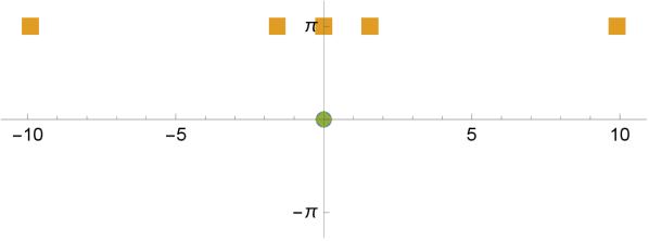
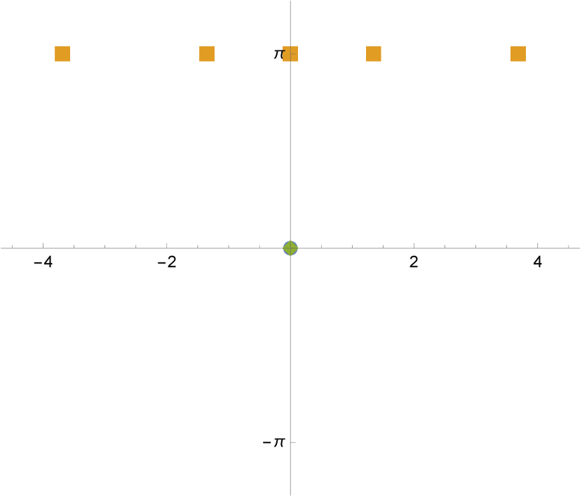
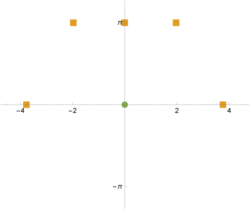
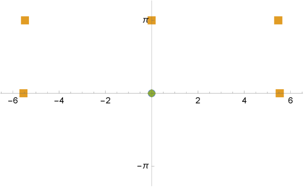
Example 1.

For each integer $n\geq 2$ , the real parameters $(b,c)$ for which ${{}_{2}F_{1}}(-n,b;c;z)$ has only real simple roots has been enumerated in [DJJ13]. The results are plotted in blue in Figure 1. The embeddedness conditions (5) are

	$\displaystyle\dot{\theta}_{1,0}>\dot{\theta}_{2,0}$	$\displaystyle\Rightarrow c<1,$
	$\displaystyle\dot{\theta}_{1,\infty}>\dot{\theta}_{2,\infty}$	$\displaystyle\Rightarrow b>-n,$
	$\displaystyle\dot{\theta}_{2,0}>\dot{\theta}_{3,0}$	$\displaystyle\Rightarrow c_{2}^{2}>-nb,$
	$\displaystyle\dot{\theta}_{2,\infty}>\dot{\theta}_{3,\infty}$	$\displaystyle\Rightarrow c_{2}^{2}>n(c_{2}+b),$

where $c_{2}=n-1-b+c$ . The region defined by these is plotted in red in Figure 1. Then non-integer parameters $(b,c)$ in the intersection of red and blue regions give rise to balanced and rigid configurations with real $q_{1,k}$ .

Refer to caption — Figure 1. The set of $b$ and $c$ for which ${{}_{2}F_{1}}(-n,b;c;z)$ has only real simple roots (blue), and for which the embeddedness conditions are satisfied (red).

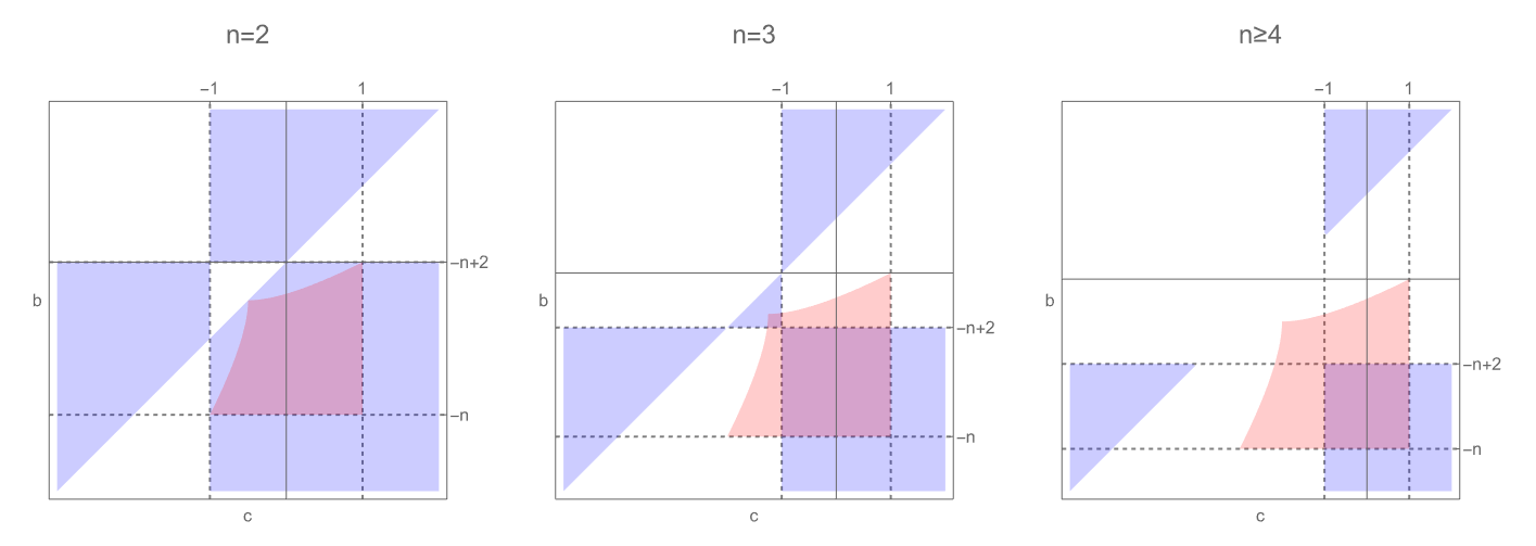
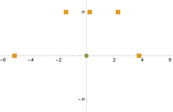
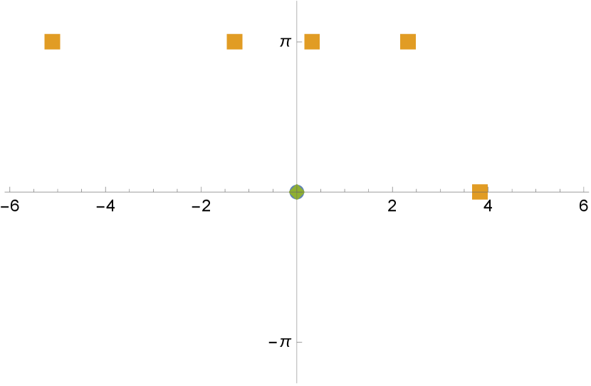
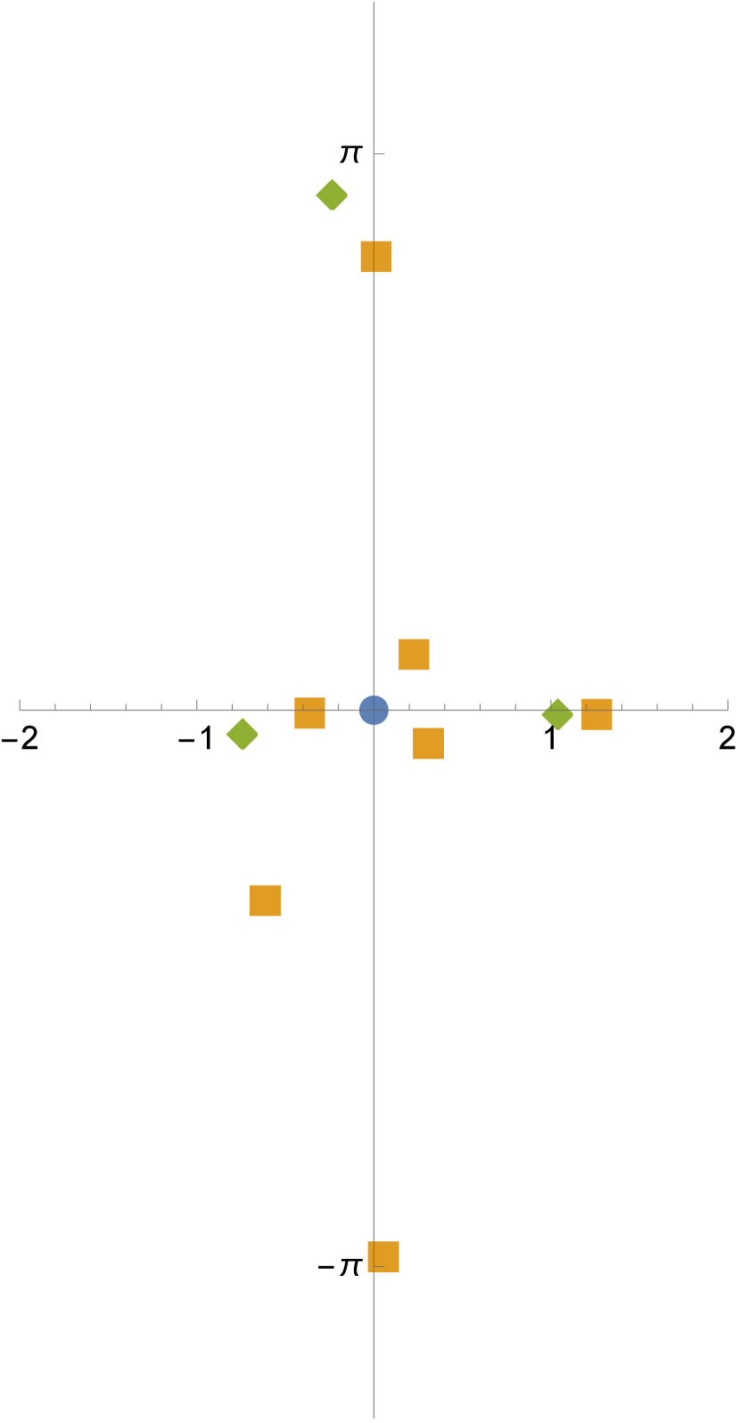
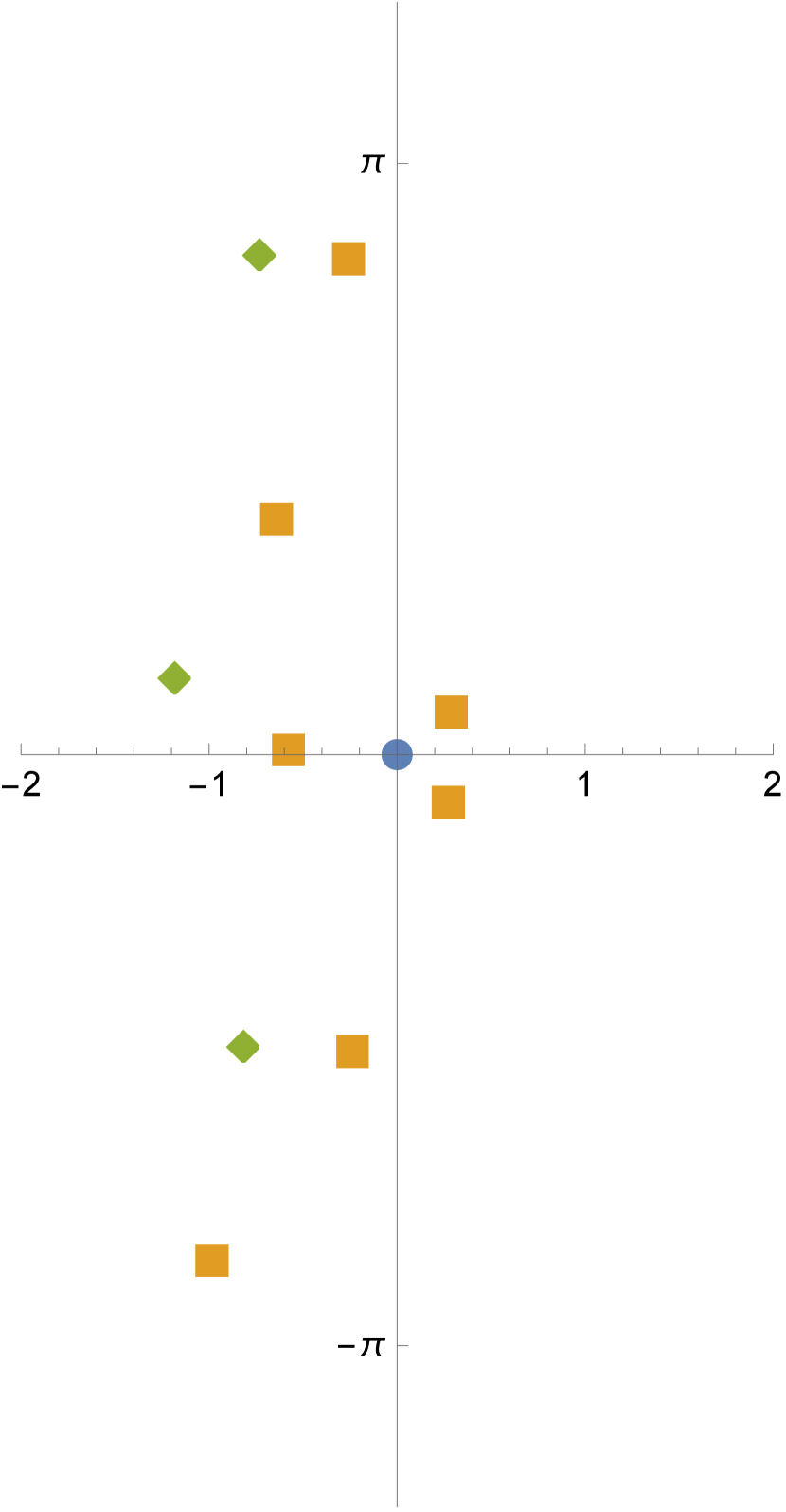
Figure 2 shows the configurations of three examples with $n=5$ . ∎

Remark 12.

As $c\to 0$ , ${{}_{2}F_{1}}(-n,b;c;z)/\Gamma(c)$ converges to a polynomial with a root at $0$ . One may interpret that, as $c$ increases across $0$ , a root moves from the interval $(-\infty,0)$ to the interval $(0,1)$ through $0$ .

When $b=1-n$ , ${{}_{2}F_{1}}(-n,b;c;z)$ becomes a polynomial of degree $n-1$ . One may interprete that, as $b$ increases across $1-n$ , a root moves from the interval $(-\infty,0)$ to the interval $(1,\infty)$ through the infinity.

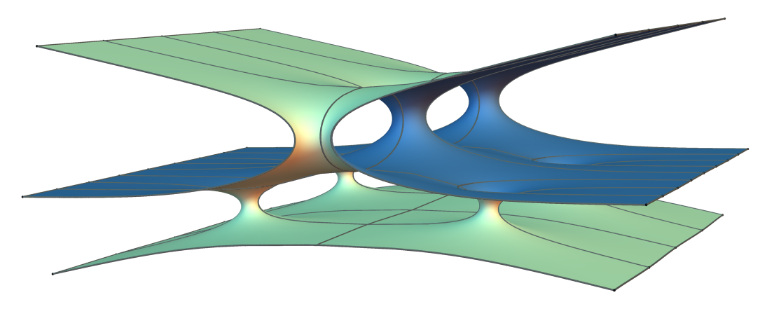
Example 2.

Assume that $b+c=1-n$ (hence $c_{2}=-2b$ ). Then by the identity

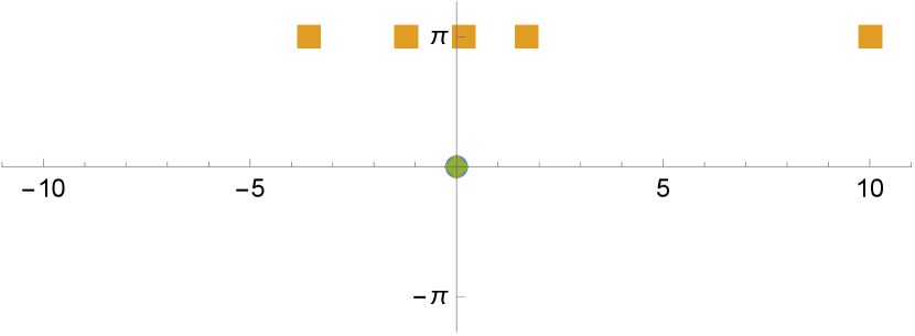
{{}_{2}F_{1}}(-n,b;c;z)=\frac{(b)_{n}}{(c)_{n}}(-z)^{n}{{}_{2}F_{1}}\left(-n,1-c-n;1-b-n;\frac{1}{z}\right),

the simple roots must be symmetrically placed. That is, if $z_{0}$ is a root, so is $1/z_{0}$ . This symmetry appears in the resulting minimal surfaces as a rotational symmetry. If the simple roots are real, the rotation reduces to a vertical reflectional. In view of Figure 1, we obtain the following concrete examples.

•

$n\geq 2$ and $0<c<1$ . In this case ${{}_{2}F_{1}}(-n,b;c;z)$ has $n$ simple negative roots. See Figure 3 for an example of this type with $n=2$ . Figure 4 shows the configurations of two examples with $n=5$ .
•

$n\geq 3$ and $-1<c<0$ , or $n=3$ and $-5/4<c<-1$ , or $n=2$ and $-1/2<c<0$ . In these case, ${{}_{2}F_{1}}(-n,b;c;z)$ has $n-2$ simple negative roots, one root $0<z_{0}<1$ , and another root $1/z_{0}>1$ . Figure 5 shows the configurations of two examples with $n=5$ . ∎

Remark 13.

Examples with six Scherk ends are parameterized by three real parameters, here by $b$ , $c$ , and the family parameter $\tau$ . We see that the relation $b+c=1-n$ imposes a rotational symmetry. It can be imagined that removing the relation would break this symmetry.

Remark 14.

The polynomial method is often used to find balanced configurations of interacting points in the plane. In minimal surface theory, it has been employed in many implementations of Traizet’s node-opening technique [Tra02b, Tra02a, TW05, Li12, CW12, Con17a, Con17b, CF22].

2.5. Surfaces with eight ends of type (1,n,1)

Theorem 5 generalizes to the following lemma with similar proof

Lemma 6.

If we fix $q_{l\pm 1,k}$ ’s and assume that $c_{l}=1$ . Then $q_{l,k}$ ’s in a balanced configuration are given by the roots of a Stieltjes polynomial $P(z)$ of degree $n_{l}$ that solves the generalized Lamé equation (a.k.a. second-order Fuchsian equation) [Mar66]

(14)		$\displaystyle P^{\prime\prime}$	$\displaystyle+\Big{(}\frac{c}{z}+\sum_{k=1}^{n_{l-1}}\frac{-c_{l-1}}{z-q_{l-1,k}}+\sum_{k=1}^{n_{l+1}}\frac{-c_{l+1}}{z-q_{l+1,k}}\Big{)}P^{\prime}$
		$\displaystyle+\Big{(}\frac{\gamma_{0}}{z}+\sum_{k=1}^{n_{l-1}}\frac{\gamma_{l-1,k}}{z-q_{l-1,k}}+\sum_{k=1}^{n_{l+1}}\frac{\gamma_{l+1,k}}{z-q_{l+1,k}}\Big{)}P=0,$

where $c=1+\dot{\theta}_{l+1,0}-\dot{\theta}_{l,0}$ , subject to conditions

	$\displaystyle\gamma_{0}+\sum_{k=1}^{n_{l-1}}\gamma_{l-1,k}+\sum_{k=1}^{n_{l+1}}\gamma_{l+1,k}$	$\displaystyle=0,$
	$\displaystyle\sum_{k=1}^{n_{l-1}}\gamma_{l-1,k}q_{l-1,k}+\sum_{k=1}^{n_{l+1}}\gamma_{l+1,k}q_{l+1,k}.$	$\displaystyle=:-n_{l}b,$

and

c-n_{l-1}c_{l-1}-n_{l+1}c_{l+1}=1-n_{l}+b.

Moreover, the matrix $(\partial F_{l,k}/\partial q_{l,j})_{1\leq j,k\leq n_{l}}$ is nonsingular as long as $b$ is not a non-positive integer bigger than $n_{l}$ .

Indeed, a root of $P(z)$ is simple if and only if it does not coincide with $0$ or any $q_{l\pm 1,k}$ . If the roots $(q_{l,k})$ of $P(z)$ are all simple, then they solve the equations [Mar66]

\sum_{1\leq k\neq j\leq n_{l}}\frac{2}{q_{l,k}-q_{l,j}}+\sum_{1\leq j\leq n_{l+1}}\frac{-c_{l+1}}{q_{l,k}-q_{l+1,j}}\\ +\sum_{1\leq j\leq n_{l-1}}\frac{-c_{l-1}}{q_{l,k}-q_{l-1,j}}+\frac{c}{q_{l,k}}=\frac{F_{l,k}}{q_{l,k}}=0,

which is exactly our balance condition; see Remark 4. Moreover, an equation system generalizing (13) has been obtained in [Hei78, §136], from which we may conclude the non-singularity of the Jacobian. In fact, there are

\binom{n_{l-1}+n_{l}+n_{l+1}-1}{n_{l-1}+n_{l+1}-1}

choices of $\gamma$ for which (14) has a polynomial solution of degree $n_{l}$ [Hei78, §135].

This observation allows us to easily construct balanced and rigid configurations of type $(1,n,1)$ : Up to reparametrizations and complex scalings, we may assume that $c_{2}=1$ and $q_{1,1}=1$ . Then $q_{3,1}$ must be real, and $(q_{2,k})_{1\leq k\leq n}$ are given by roots of a Heun polynomial. Such a configuration depends locally on four real parameters, namely $q_{3,1}$ , $c_{1}$ , $c_{3}$ and $c$ (or $b$ ). When these are given, we have $n+1$ Heun polynomials, each of which gives balanced positions of $q_{2,k}$ ’s. For each of the Heun polynomials $P$ , we have

	$\displaystyle\dot{\theta}_{2,0}-\dot{\theta}_{1,0}$	$\displaystyle=\frac{P^{\prime}(1)}{P(1)}-c_{1},$
	$\displaystyle\dot{\theta}_{3,0}-\dot{\theta}_{2,0}$	$\displaystyle=c-1=b+c_{1}+c_{3}-n,$
	$\displaystyle\dot{\theta}_{4,0}-\dot{\theta}_{3,0}$	$\displaystyle=\frac{P^{\prime}(q_{3,1})}{P(q_{3,1})}-c_{3}.$

Together with the family parameter $\tau$ , the surface depends locally on five parameters, which is expected because there are eight ends.

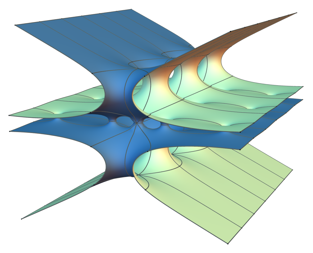
Example 3 (Symmetric examples).

When $q_{3,1}=q_{1,1}=1$ , the Heun polynomial reduces to a hypergeometric polynomial ${{}_{2}F_{1}}(-n,b;c;z)$ , where $c_{1}+c_{3}=n-1-b+c$ . Assume further that $b+c=1-n$ , so $c_{1}+c_{3}=-2b$ . This imposes a symmetry in the configuration. Because $(c_{1}+c_{3})P^{\prime}(1)/P(1)=-nb$ , the embeddedness conditions simplify to

c_{1}>n/2,\quad c_{3}>n/2,\quad 1-n/2<c<1,\quad-n<b<-n/2.

As explained in Example 2, the hypergeometric polynomial has real roots if $b$ and $c$ lie in the blue regions of Figure 1. More specifically:

•

When $n\geq 2$ and $0<c<1$ , ${{}_{2}F_{1}}(-n,b;c;z)$ has $n$ simple negative roots. See Figure 6 for an example with $n=5$ .
•

When $n\geq 4$ and $-1<c<0$ , or $n=3$ and $-1/2<c<0$ , ${{}_{2}F_{1}}(-n,b;c;z)$ has $n-2$ simple negative roots, one root $0<z_{0}<1$ , and another root $1/z_{0}>1$ . ∎

Example 4 (Offset handles).

There are embedded examples in which the handles are not symmetrically placed. For instance, one balanced configuration of type $(1,2,1)$ is given by

	$\displaystyle q_{3,1}=2/3,$	$\displaystyle q_{2,1}=-1/3,$	$\displaystyle q_{2,2}=-23,$
	$\displaystyle c_{1}=8/5,$	$\displaystyle c_{3}=4189/2890,$	$\displaystyle b=-9857/8670,$

so $c=3956/4335$ . ∎

2.6. Concatenating surfaces of type (1,n,1)

We describe a family of examples in the same spirit as [Tra02a, Proposition 2.3]. Assume that we are in possession of $R$ configurations of type $(1,n^{(r)},1)$ , $n^{(r)}>1$ , $1\leq r\leq R$ . In the following, we use superscript $(r)$ to denote the parameters of the $r$ -th configuration. Up to reparameterizations and complex scalings, we may assume that $c_{2}^{(r)}=1$ and $q_{1,1}^{(r)}=1$ . Then we may concatenate these configurations into one of type

(1,n_{2},1,n_{4},1,\cdots,1,n_{2R},1)

such that $q_{1,1}=1$ , $c_{1}=1$ , and for $1\leq r\leq R$ , we have $n_{2r}=n^{(r)}$ ,

	$\displaystyle q_{2r,k}$	$\displaystyle=q_{2r-1,1}q_{2,k}^{(r)},$	$\displaystyle q_{2r+1,1}$	$\displaystyle=q_{2r-1,1}q_{3,1}^{(r)},$
	$\displaystyle c_{2r}$	$\displaystyle=c_{2r-1}/c_{1}^{(r)},$	$\displaystyle c_{2r+1}$	$\displaystyle=c_{2r-1}c_{3}^{(r)}/c_{1}^{(r)},$

and

\dot{\theta}_{2r+1,0}-\dot{\theta}_{2r,0}=c_{2r}(c^{(r)}-1).

The balance of even layers then follows from the balance of each sub-configuration. The balance of odd layers leads to

\dot{\theta}_{2r,0}-\dot{\theta}_{2r-1,0}=c_{2r}(\dot{\theta}_{2,0}^{(r)}-\dot{\theta}_{1,0}^{(r)}+c_{1}^{(r)})+c_{2r-2}(\dot{\theta}_{4,0}^{(r-1)}-\dot{\theta}_{3,0}^{(r-1)}+c_{3}^{(r-1)})-c_{2r-1}

for $1\leq r\leq R+1$ . As expected, such a configuration depends locally on $4R$ real parameters, namely $q_{3,1}^{(r)}$ , $c_{1}^{(r)}$ , $c_{3}^{(r)}$ , and $c^{(r)}$ , $1\leq r\leq R$ .

We may impose symmetry by assuming that $q_{3,1}^{(r)}=1$ , so $q_{2r+1,1}=1$ for all $0\leq r\leq R$ , and that $b^{(r)}+c^{(r)}=1-n^{(r)}$ , so $c_{1}^{(r)}+c_{3}^{(r)}=n^{(r)}-1-b^{(r)}+c^{(r)}=-2b^{(r)}$ . Then $q_{2r,k}=q_{2,k}^{(r)}$ , $1\leq k\leq n^{(r)}$ , are given by the roots of ${{}_{2}F_{1}}(-n^{(r)},b^{(r)};c^{(r)};z)$ , $1\leq r\leq R$ . Because

\dot{\theta}_{2,0}^{(r)}-\dot{\theta}_{1,0}^{(r)}+c_{1}^{(r)}=\dot{\theta}_{4,0}^{(r)}-\dot{\theta}_{3,0}^{(r)}+c_{1}^{(r)}=n^{(r)}/2,

the embeddedness conditions simplify to

2n_{l}c_{l}>n_{l-1}c_{l-1}+n_{l+1}c_{l+1}

for $1\leq l\leq L$ under the condition that $n_{0}=n_{L+1}=0$ . That is, the sequence $(n_{l}c_{l})_{1\leq l\leq L}$ must be concave. For even $l$ , the concavity implies that $b^{(r)}>-n$ hence $c^{(r)}<1$ for all $1\leq r\leq R$ . We may choose, for instance, $n_{l}c_{l}=\ln(1+l)$ or $n_{l}c_{l}=(\exp l-1)/\exp(l-1)$ to obtain embedded minimal surfaces.

Remark 15.

We can also append a configuration of type $(1,n^{(r)})$ to the sequence of $(1,n^{(r)},1)$ -configurations to obtain a configuration of type

(1,n_{2},1,n_{4},1,\ldots,1,n_{2R-2},1,n_{2R}),

where the $q_{l,k},c_{l},\dot{\theta}_{l,0}$ terms are defined as above. Therefore, an embedded example of any genus with any even number ( $>2$ ) of ends can be constructed.

2.7. Numerical examples

The balance equations can be combined into one differential equation that is much easier to solve. A solution of this differential equation corresponds to a lot of balance configurations that are equivalent by permuting the locations of the nodes.

Lemma 7.

Let $L$ be a positive integer, $n_{1},n_{2},\ldots,n_{L}\in\mathbb{N}$ , and suppose $\{q_{l,k}\}$ is a configuration such that the $q_{l,k}$ are distinct. Let

P_{l}(z)=\prod_{k=1}^{n_{l}}(z-q_{l,k}),\quad P(z)=\prod_{l=1}^{L}P_{l}(z),\quad P_{0}(z)=P_{L+1}(z)=1,\\

and

\begin{split}\mathcal{F}P(z)=\sum_{l=1}^{L}&\left(\frac{c_{l}^{2}zP_{l}^{\prime\prime}(z)P(z)}{P_{l}(z)}-\frac{c_{l}c_{l+1}zP_{l}^{\prime}(z)P_{l+1}^{\prime}(z)P(z)}{P_{l}(z)P_{l+1}(z)}\right.\\ &\hskip 14.45377pt\left.+\left(c_{l}^{2}+c_{l}(\dot{\theta}_{l+1,0}-\dot{\theta}_{l,0})\right)\frac{P_{l}^{\prime}(z)P(z)}{P_{l}(z)}\right).\end{split}

Then the configuration $\{q_{l,k}\}$ is balanced if and only if $\mathcal{F}P(z)\equiv 0$ .

Proof.

We have seen that,

\frac{P_{l}^{\prime\prime}(q_{l,k})}{P^{\prime}_{l}(q_{l,k})}=\sum_{1\leq k\neq j\leq n_{l}}\frac{2}{q_{l,k}-q_{l,j}},\qquad\frac{P_{l\pm 1}^{\prime}(q_{l,k})}{P_{l\pm 1}(q_{l,k})}=\sum_{j=1}^{n_{l\pm 1}}\frac{1}{q_{l,k}-q_{l\pm 1,j}}.

Define

F_{l}(z)=\frac{c_{l}^{2}zP_{l}^{\prime\prime}(z)}{P_{l}^{\prime}(z)}-\frac{c_{l}c_{l+1}zP_{l+1}^{\prime}(z)}{P_{l+1}(z)}-\frac{c_{l}c_{l-1}zP_{l-1}^{\prime}(z)}{P_{l-1}(z)}+c_{l}^{2}+c_{l}(\dot{\theta}_{l+1,0}-\dot{\theta}_{l,0}).

Then $F_{l,k}=F_{l}(q_{l,k})$ . Set

\begin{split}Q_{l}(z)&=\frac{P_{l}^{\prime}(z)P(z)}{P_{l}(z)}F_{l}(z)\\ &=\frac{c_{l}^{2}zP_{l}^{\prime\prime}(z)P(z)}{P_{l}(z)}-\frac{c_{l}c_{l+1}zP_{l}^{\prime}(z)P_{l+1}^{\prime}(z)P(z)}{P_{l}(z)P_{l+1}(z)}-\frac{c_{l}c_{l-1}zP_{l-1}^{\prime}(z)P_{l}^{\prime}(z)P(z)}{P_{l-1}(z)P_{l}(z)}\\ &\hskip 14.45377pt+\left(c_{l}^{2}+c_{l}(\dot{\theta}_{l+1,0}-\dot{\theta}_{l,0})\right)\frac{P_{l}^{\prime}(z)P(z)}{P_{l}(z)}.\end{split}

Then $F_{l,k}=0$ if and only if $Q_{l}(q_{l,k})=0$ .

Now observe that $Q_{l}(z)$ and $Q(z)=\mathcal{F}P(z)$ are polynomials with degree strictly less than

\deg P=N=\sum_{l=1}^{L}n_{l},

and $Q(q_{l,k})=Q_{l}(q_{l,k})$ for $1\leq k\leq n_{l}$ and $1\leq l\leq L$ . If $Q\equiv 0$ then $Q_{l}(q_{l,k})=0$ and so $\{q_{l,k}\}$ is a balanced configuration. If $\{q_{l,k}\}$ is a balanced configuration then $Q(q_{l,k})=Q_{l}(q_{l,k})=F_{l,k}=0$ . Hence, $Q$ has at least $N$ distinct roots. Since the degree of $Q$ is strictly less than $N$ , we must have $Q\equiv 0$ . ∎

It is relatively easy to numerically solve $\mathcal{F}P(z)\equiv 0$ as long as we don’t have too many levels and necks. So we use this lemma to find balanced configurations. Since all previous examples admit a horizontal reflection symmetry, we are most interested examples without this symmetry, or with no non-trivial symmetry at all.

Figure 7 shows an example with $L=3$ ,

	$\displaystyle n_{1}=1,n_{2}=3,n_{3}=2$
	$\displaystyle c_{1}=2,c_{2}=1,c_{3}=13/16$
	$\displaystyle\theta_{1,0}=0,\theta_{2,0}=-1/2,\theta_{3,0}=-27/16,\theta_{4,0}=-29/16.$

This configuration corresponds to an embedded minimal surface with eight ends and genus three in the quotient. It has no horizontal reflectional symmetry, but does have a rotational symmetry.

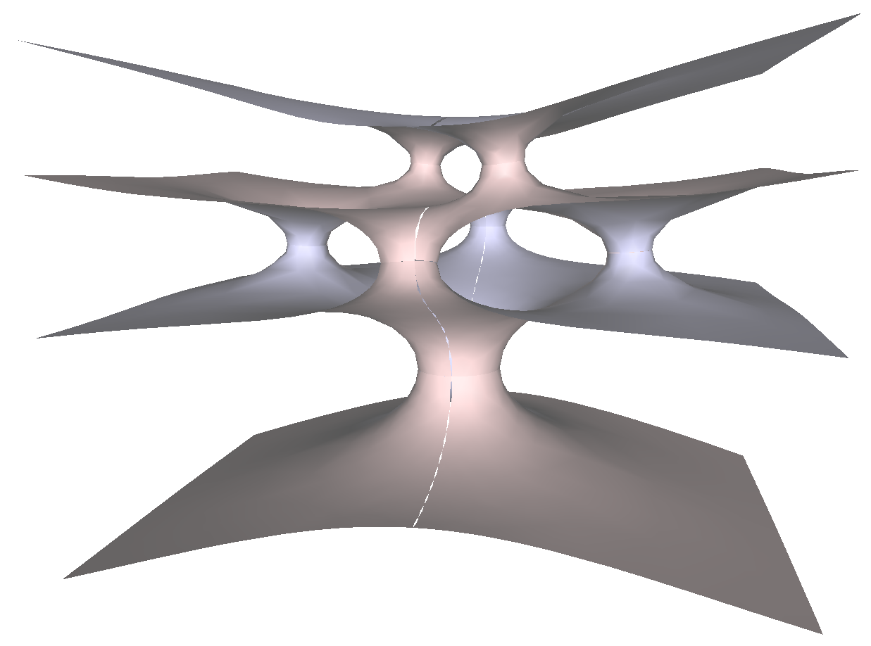
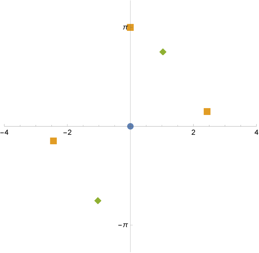
Figure 8 shows two examples with $L=3$ ,

	$\displaystyle n_{1}=1,n_{2}=4,n_{3}=3$
	$\displaystyle c_{1}=7/2,c_{2}=1,c_{3}=3/4$
	$\displaystyle\theta_{1,0}=0,\theta_{2,0}=-2,\theta_{3,0}=-13/5,\theta_{4,0}=-541/180.$

These configurations correspond to embedded minimal surfaces with eight ends and genus five in the quotient, with no nontrivial symmetry.

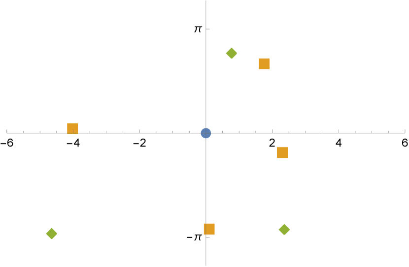
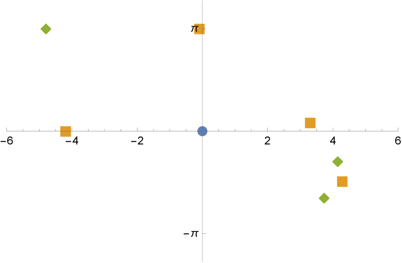
Figure 9 shows two examples with $L=3$ ,

	$\displaystyle n_{1}=1,n_{2}=7,n_{3}=3,$
	$\displaystyle c_{1}=17/7,c_{2}=1,c_{3}=3/2,$
	$\displaystyle\theta_{1,0}=0,\theta_{2,0}=-1/2,\theta_{3,0}=-3/2,\theta_{4,0}=-2468/441.$

These configurations correspond to embedded minimal surfaces with eight ends and genus eight in the quotient, with no nontrivial symmetry.

3. Construction

3.1. Opening nodes

To each vertical plane is associated a punctured complex plane $\mathbb{C}^{\times}_{l}\simeq\mathbb{C}\setminus\{0\}$ , $1\leq l\leq L+1$ . They can be seen as Riemann spheres $\hat{\mathbb{C}}_{l}\simeq\mathbb{C}\cup\{\infty\}$ with two fixed punctures at $p_{l,0}=0$ and $p_{l,\infty}=\infty$ , corresponding to the two ends.

To each neck is associated a puncture $p^{\circ}_{l,k}\in\mathbb{C}^{\times}_{l}$ and a puncture $p^{\prime\circ}_{l,k}\in\mathbb{C}^{\times}_{l+1}$ . Our initial surface at $\tau=0$ is the noded Riemann surface $\Sigma_{0}$ obtained by identifying $p^{\circ}_{l,k}$ and $p^{\prime\circ}_{l,k}$ for $1\leq l\leq L$ and $1\leq k\leq n_{l}$ .

As $\tau$ increases, we open the nodes into necks as follows: Fix local coordinates $w_{l,0}=z$ in the neighborhood of $0\in\hat{\mathbb{C}}_{l}$ and $w_{l,\infty}=1/z$ in the neighborhood of $\infty\in\hat{\mathbb{C}}_{l}$ . For each neck, we consider parameters $(p_{l,k},p^{\prime}_{l,k})$ in the neighborhoods of $(p^{\circ}_{l,k},p^{\prime\circ}_{l,k})$ and local coordinates

w_{l,k}=\ln(z/p_{l,k})\quad\text{and}\quad w^{\prime}_{l,k}=\ln(z/p^{\prime}_{l,k})

in a neighborhood of $p_{l,k}$ and $p^{\prime}_{l,k}$ , respectively. In this paper, the branch cut of $\ln(z)$ is along the negative real axis, and we use the principal value of $\ln(z)$ with imaginary part in the interval $(-\pi,\pi]$ .

As we only open finitely many necks, we may choose $\delta>0$ independent of $k$ and $l$ such that the disks

	$\displaystyle\|w_{h}\|<2\delta,\qquad h\in\mathsf{H}\quad(=[1,L+1]\times\{0,\infty\}),$
	$\displaystyle\|w_{l,k}\|<2\delta\quad\text{and}\quad\|w^{\prime}_{l,k}\|<2\delta,\qquad 1\leq l\leq L,1\leq k\leq n_{k}$

are all disjoint. For parameters $t=(t_{l,k})_{1\leq l\leq L,1\leq k\leq n_{l}}$ in a neighborhood of $0$ with $|t_{l,k}|<\delta^{2}$ , we remove the disks

|w_{l,k}|<|t_{l,k}|/\delta\quad\text{and}\quad|w^{\prime}_{l,k}|<|t_{l,k}|/\delta

and identify the annuli

|t_{l,k}|/\delta\leq|w_{l,k}|\leq\delta\quad\text{and}\quad|t_{l,k}|/\delta\leq|w^{\prime}_{l,k}|\leq\delta

w_{l,k}w^{\prime}_{l,k}=t_{l,k}.

If $t_{l,k}\neq 0$ for all $1\leq l\leq L$ and $1\leq k\leq n_{l}$ , we obtain a Riemann surface denoted by $\Sigma_{t}$ .

3.2. Weierstrass data

We construct a conformal minimal immersion using the Weierstrass parameterization in the form

z\mapsto\operatorname{Re}\int^{z}(\Phi_{1},\Phi_{2},\Phi_{3}),

where $\Phi_{i}$ are meromorphic 1-forms on $\Sigma_{t}$ satisfying the conformality equation

(15)

Q:=\Phi_{1}^{2}+\Phi_{2}^{2}+\Phi_{3}^{2}=0.

3.2.1. A-periods

We consider the following fixed domains in all $\Sigma_{t}$ :

	$\displaystyle U_{l,\delta}=\{z\in\hat{\mathbb{C}}_{v}\colon$	$\displaystyle\|w^{\circ}_{l,k}(z)\|>\delta/2\quad\forall 1\leq k\leq n_{l}\quad\text{if}\;1\leq l\leq L$
	and	$\displaystyle\|w^{\prime\circ}_{l,k}(z)\|>\delta/2\quad\forall 1\leq k\leq n_{l-1}\quad\text{if}\;2\leq l\leq L+1\}$

and $U_{\delta}=\bigsqcup_{1\leq l\leq L}U_{l,\delta}$ .

Let $A_{l,k}$ denote a small counterclockwise circle in $U_{l,\delta}$ around $p_{l,k}$ ; it is then homologous in $\Sigma_{t}$ to a clockwise circle in $U_{l+1,\delta}$ around $p^{\prime}_{l,k}$ . Moreover, let $A_{l,0}$ (resp. $A_{l,\infty}$ ) denote a small counterclockwise circle in $U_{l,\delta}$ around $0$ (resp. $\infty$ ).

Recall that the vertical period vector is assumed to be $(0,0,2\pi)$ , so we need to solve the A-period problems

\operatorname{Re}\int_{A_{h}}(\Phi_{1},\Phi_{2},\Phi_{3})=(0,0,2\pi\sigma_{h})\quad\text{and}\quad\operatorname{Re}\int_{A_{l,k}}(\Phi_{1},\Phi_{2},\Phi_{3})=(0,0,0)

for $h\in\mathsf{H}$ , $1\leq l\leq L$ , and $1\leq k\leq n_{l}$ . Here, the orientation $\sigma_{h}=\pm 1$ satisfies

\sigma_{h}=-\sigma_{\varsigma(h)},

where the “counterclockwise rotation” $\varsigma$ on $\mathsf{H}$ is defined by

(16)

\begin{cases}\varsigma(0_{l})=0_{l-1},&2\leq l\leq L+1,\\ \varsigma(0_{1})=\infty_{1},\\ \varsigma(\infty_{l})=\infty_{l+1},&1\leq l\leq L,\\ \varsigma(\infty_{L+1})=0_{L+1}.\end{cases}

In particular, we have $\sigma_{l,0}=-\sigma_{l,\infty}$ for all $1\leq l\leq L+1$ .

Recall that the surface tends to an $(L+1)$ -sheeted $xz$ -plane in the limit $\tau\to 0$ . So we define the meromorphic functions $\Phi_{1}$ , $\Phi_{2}$ and $\Phi_{3}$ as the unique regular 1-forms on $\Sigma_{t}$ (see [Tra13, §8]) with simple poles at $p_{h}$ , $h\in\mathsf{H}$ , and the A-periods

	$\displaystyle\int_{A_{h}}{(\Phi_{1},\widetilde{\Phi}_{2},\Phi_{3})}$	$\displaystyle=2\pi{\rm i}(\alpha_{h},\beta_{h},\gamma_{h}-{\rm i}\sigma_{h}),$	$\displaystyle h\in\mathsf{H},$
	$\displaystyle\int_{A_{l,k}}(\Phi_{1},\widetilde{\Phi}_{2},\Phi_{3})$	$\displaystyle=2\pi{\rm i}(\alpha_{l,k},\beta_{l,k},\gamma_{l,k}),$	$\displaystyle 1\leq l\leq L,1\leq k\leq n_{l},$

where $\Phi_{2}=\tau\widetilde{\Phi}_{2}$ and, by Residue Theorem, it is necessary that

(17)	$\displaystyle\alpha_{l,0}+\alpha_{l,\infty}+\sum_{1\leq k\leq n_{l}}\alpha_{l,k}-\sum_{1\leq k\leq n_{l-1}}\alpha_{l-1,k}$	$\displaystyle=0,$
(18)	$\displaystyle\beta_{l,0}+\beta_{l,\infty}+\sum_{1\leq k\leq n_{l}}\beta_{l,k}-\sum_{1\leq k\leq n_{l-1}}\beta_{l-1,k}$	$\displaystyle=0,$
(19)	$\displaystyle\gamma_{l,0}+\gamma_{l,\infty}+\sum_{1\leq k\leq n_{l}}\gamma_{l,k}-\sum_{1\leq k\leq n_{l-1}}\gamma_{l-1,k}$	$\displaystyle=0,$

for $1\leq l\leq L+1$ . Then the A-period problems are solved by definition.

3.2.2. Balance of ends

Summing up (18) over $l$ gives

(20)

\sum_{h\in\mathsf{H}}\beta_{h}=0,

which we use to replace Equation (18) with $l=L+1$ .

In this paper, the punctures $p_{l,0}$ and $p_{l,\infty}$ correspond to Scherk-type ends. Hence we fix

(21)

\alpha^{2}_{h}+\tau^{2}\beta_{h}^{2}\equiv 1\quad\text{and}\quad\gamma_{h}\equiv 0

for all $h\in\mathsf{H}$ , so that (the stereographic projection of) the Gauss map $G=-(\Phi_{1}+{\rm i}\Phi_{2})/\Phi_{3}$ extends holomorphically to the punctures $p_{h}$ with unitary values. Then Equations (19) are not independent: if it is solved for $1\leq l\leq L$ , it is automatically solved for $l=L+1$ .

In particular, at $\tau=0$ , we have $\alpha_{h}^{2}=1$ . In view of the orientation of the ends, we choose $\alpha_{l,0}=1$ and $\alpha_{l,\infty}=-1$ so that $G(p_{l,\infty})=G(p_{l,0})={\rm i}\sigma_{l,0}$ .

Summing up (17) over $l$ gives

(22)

\sum_{1\leq l\leq L+1}\Big{(}\sqrt{1-\tau^{2}\beta_{l,\infty}^{2}}-\sqrt{1-\tau^{2}\beta_{l,0}^{2}}\Big{)}=0,

which we use to replace Equation (17) with $l=L+1$ .

Remark 16.

The conditions (20) and (22) are disguises of the balance condition of Scherk ends, namely that the unit vectors in their directions should sum up to $0$ .

3.2.3. B-periods

For $1\leq l\leq L+1$ , we fix a point $O_{l}\in U_{l,\delta}$ . For every $1\leq l\leq L$ and $1\leq k\leq n_{l}$ and $t_{l,k}\neq 0$ , let $B_{l,k}$ be the concatenation of

(1)

a path in $U_{l,\delta}$ from $O_{l}$ to $w_{l,k}=\delta$ ,
(2)

the path parameterized by $w_{l,k}=\delta^{1-2s}\,t_{l,k}^{s}$ for $s\in[0,1]$ , from $w_{l,k}=\delta$ to $w_{l,k}=t_{h}/\delta$ , which is identified with $w^{\prime}_{l,k}=\delta$ , and
(3)

a path in $U_{l+1,\delta}$ from $w^{\prime}_{l,k}=\delta$ to $O_{l+1}$ .

We need to solve the B-period problem, namely that

(23)

\operatorname{Re}\int_{B_{l,k}}(\Phi_{1},\Phi_{2},\Phi_{3})=\operatorname{Re}\int_{B_{l,1}}(\Phi_{1},\Phi_{2},\Phi_{3}).

3.2.4. Conformality

Lemma 8.

For $t$ sufficiently close to $0$ , the conformality condition (15) is equivalent to

(24)	$\displaystyle\mathfrak{G}_{l,k}:=\int_{A_{l,k}}\frac{w_{l,k}Q}{dw_{l,k}}$	$\displaystyle=0,\quad 1\leq l\leq L,\quad 1\leq k\leq n_{l},$
(25)	$\displaystyle\mathfrak{F}_{l,k}:=\int_{A_{l,k}}\frac{Q}{dw_{l,k}}$	$\displaystyle=0,\quad 1\leq l\leq L,\quad 2\leq k\leq n_{l},$
(26)	$\displaystyle\mathfrak{F}^{\prime}_{l,k}:=\int_{A^{\prime}_{l,k}}\frac{Q}{dw^{\prime}_{l,k}}$	$\displaystyle=0,\quad 1\leq l\leq L,\quad 1+\delta_{l,L}\leq k\leq n_{l},$

where $A^{\prime}_{l,k}$ in (26) denotes a small counterclockwise circle in $U_{l+1,\delta}$ around $p^{\prime}_{l,k}$ (hence homologous to $-A_{l,k}$ ), and $\delta_{l,L}=1$ if $l=L$ and $0$ otherwise.

Proof.

By our choice of $\alpha_{h}$ and $\gamma_{h}$ , the quadratic differential $Q$ has at most simple poles at the $2L+2$ punctures $p_{h}$ , $h\in\mathsf{H}$ . The space of such quadratic differentials is of complex dimension $3(N-L)-3+(2L+2)=3N-L-1$ . We will prove that

Q\mapsto(\mathfrak{G},\mathfrak{F},\mathfrak{F}^{\prime})

is an isomorphism. We prove the claim at $t=0$ ; then the claim follows by continuity.

Consider $Q$ in the kernel. Recall from [Tra08] that a regular quadratic differential on $\Sigma_{0}$ has at most double poles at the nodes $p_{l,k}$ and $p^{\prime}_{l,k}$ . Then (24) guarantees that $Q$ has at most simple poles at the nodes. By (25) and (26), $Q$ may only have simple poles at $p_{l,1}\in\mathbb{C}^{\times}_{l}$ , $1\leq l\leq L$ , and $p^{\prime}_{L,1}\in\mathbb{C}^{\times}_{L+1}$ . So, on each Riemann sphere $\hat{\mathbb{C}}_{l}$ , $Q$ is a quadratic differential with at most simple poles at three punctures; the other two being $0$ , $\infty$ . But such a quadratic differential must be $0$ . ∎

3.3. Using the Implicit Function Theorem

All parameters varies in a neighborhood of their central values, denoted by a superscript $\circ$ . We will see that

\beta^{\circ}_{h}=\dot{\theta}_{h},\;\alpha^{\circ}_{l,k}=\gamma^{\circ}_{l,k}=0,\;\beta^{\circ}_{l,k}=-c_{l},\;p^{\prime\circ}_{l,k}=\overline{p_{l,k}}.

Let us first solve Equations (20) and (22).

Proposition 9.

Given a configuration $(q,\dot{\theta})$ such that $\Theta_{1}=\Theta_{2}=0$ . For $\tau$ sufficiently small and $\beta_{h}$ close to $\beta^{\circ}_{h}=\dot{\theta}_{h}$ , the solutions $(\tau,\beta)$ to Equations (20) and (22) form a smooth manifold of dimension $2L+1$ .

Proof.

At $\tau=0$ , Equation (20) is solved by $\beta^{\circ}_{h}=\dot{\theta}_{h}$ if $\Theta_{1}=0$ . Taking the derivative of (22) with respect to $\tau^{2}$ gives

(27)

\sum_{1\leq l\leq L+1}\frac{\beta_{l,\infty}^{2}-\beta_{l,0}^{2}}{2}=0,

which is solved by $\beta^{\circ}_{h}=\dot{\theta}_{h}$ if $\Theta_{2}=0$ . The proposition then follows from Lemma 1 and the Implicit Function Theorem. ∎

From now on, we assume that the parameters $(\tau,(\beta_{h})_{h\in\mathsf{H}})$ are solutions to Equations (20) and (22) in a neighborhood of $(0,\dot{\theta})$ .

3.3.1. Solving conformality problems

Proposition 10.

For $\tau$ sufficiently small and $\beta_{l,k}$ , $p_{l,k}$ , and $p^{\prime}_{l,k}$ in a neighborhood of their central values, there exist unique values of $t_{l,k}$ , $\alpha_{l,k}$ , and $\gamma_{l,k}$ , depending real-analytically on $(\tau^{2},\beta,p,p^{\prime})$ , such that the balance equations (17) and (19) with $1\leq l\leq L$ and the conformality Equations (24) and (25) are solved. Moreover, at $\tau=0$ , we have $t_{l,k}=0$ , $\alpha_{l,k}=\gamma_{l,k}=0$ ,

\frac{\partial t_{l,k}}{\partial(\tau^{2})}=\frac{1}{4}\beta_{l,k}^{2},

and, for $2\leq k\leq n_{l}$ ,

(28)

\frac{\partial}{\partial(\tau^{2})}(\alpha_{l,k}-{\rm i}\sigma_{l,0}\gamma_{l,k})=-\frac{1}{2}\operatorname{Res}\left(\frac{\widetilde{\Phi}_{2}^{2}}{dw_{l,k}},p_{l,k}\right)=-\frac{1}{2}\operatorname{Res}\left(\frac{z\widetilde{\Phi}_{2}^{2}}{dz},p_{l,k}\right).

Note that, according to this proposition, if $\beta^{\circ}_{l,k}\neq 0$ , then $t_{l,k}>0$ for sufficiently small $\tau$ .

Proof.

At $\tau=0$ , for $2\leq k\leq n_{l}$ we have

\mathfrak{G}_{l,k}=\int_{A_{l,k}}\frac{w_{l,k}Q}{dw_{l,k}}=2\pi{\rm i}(\alpha_{l,k}^{2}+\gamma_{l,k}^{2})=0

which vanishes when

\alpha_{l,k}=\gamma_{l,k}=0.

Recall that $\alpha_{h}=\pm 1$ at $\tau=0$ and that $\gamma_{h}\equiv 0$ . Then by Residue Theorem, we have

\alpha_{l,1}=\gamma_{l,1}=0.

As a consequence, we have at $\tau=0$

\Phi^{\circ}_{1}=dz/z,\quad\Phi^{\circ}_{2}=0,\quad\text{and}\quad\Phi^{\circ}_{3}=-{\rm i}\sigma_{l,0}dz/z,

so $Q=0$ as we expect.

We then compute the partial derivatives at $\tau=0$

	$\displaystyle\frac{\partial}{\partial\alpha_{l,k}}\mathfrak{F}_{l,k}$	$\displaystyle=\int_{A_{l,k}}2\frac{\Phi^{\circ}_{1}}{dw_{l,k}}\frac{\partial\Phi_{1}}{\partial\alpha_{l,k}}\bigg{\|}_{\tau=0}=\int_{A_{l,k}}2\frac{dz/z}{dz/p}\frac{dz}{z-p_{l,k}}=4\pi{\rm i}\,,$
	$\displaystyle\frac{\partial}{\partial\gamma_{l,k}}\mathfrak{F}_{l,k}$	$\displaystyle=\int_{A_{l,k}}2\frac{\Phi^{\circ}_{3}}{dw_{l,k}}\frac{\partial\Phi_{3}}{\partial\gamma_{l,k}}\bigg{\|}_{\tau=0}=\int_{A_{l,k}}-2i\sigma_{l,0}\frac{dz/z}{dz/p}\frac{dz}{z-p_{l,k}}=4\pi\sigma_{l,0}\,,$
	$\displaystyle\frac{\partial}{\partial t_{l,k}}\mathfrak{G}_{l,k}$	$\displaystyle=\int_{A_{l,k}}\frac{2w_{l,k}}{dw_{l,k}}\Big{(}\Phi^{\circ}_{1}\frac{\partial\Phi^{\circ}_{1}}{\partial t_{l,k}}+\Phi^{\circ}_{3}\frac{\partial\Phi^{\circ}_{3}}{\partial t_{l,k}}\Big{)}$
		$\displaystyle=\frac{-1}{\pi{\rm i}}\Big{(}\int_{A_{l,k}}\frac{\Phi^{\circ}_{1}}{w_{l,k}}\int_{A^{\prime}_{l,k}}\frac{\Phi^{\circ}_{1}}{w^{\prime}_{l,k}}+\int_{A_{l,k}}\frac{\Phi^{\circ}_{3}}{w_{l,k}}\int_{A^{\prime}_{l,k}}\frac{\Phi^{\circ}_{3}}{w^{\prime}_{l,k}}\Big{)}\quad\text{\cite[cite]{[\@@bibref{}{traizet2008}{}{}, Lemma~{}3]}}$
		$\displaystyle=-8\pi{\rm i}.$

All other partial derivatives vanish. Therefore, by the Implicit Function Theorem, there exist unique values of $\alpha_{l,k}$ , $\gamma_{l,k}$ (with $2\leq k\leq n_{l}$ ), and $t_{l,k}$ (with $1\leq k\leq n_{l}$ ) that solve the conformality Equations (24) and (25). Recall that $\alpha_{h}$ are determined by (21). Then $\alpha_{l,1}$ and $\gamma_{l,1}$ are uniquely determined by the linear balance equations (17) and (19).

Moreover,

\frac{\partial}{\partial(\tau^{2})}\mathfrak{F}_{l,k}=\int_{A_{l,k}}\frac{\widetilde{\Phi}_{2}^{2}}{dw_{l,k}},\quad\frac{\partial}{\partial(\tau^{2})}\mathfrak{G}_{l,k}=2\pi{\rm i}\beta_{l,k}^{2}.

Hence the total derivatives

\frac{d}{d(\tau^{2})}\mathfrak{F}_{l,k}=4\pi{\rm i}\frac{\partial\alpha_{l,k}}{\partial(\tau^{2})}+4\pi\sigma_{l,0}\frac{\partial\gamma_{l,k}}{\partial(\tau^{2})}+2\pi{\rm i}\operatorname{Res}\left(\frac{\widetilde{\Phi}_{2}^{2}}{dw_{l,k}},p_{l,k}\right)=0

and

\frac{d}{d(\tau^{2})}\int_{A_{l,k}}\mathfrak{G}_{l,k}=-8\pi{\rm i}\frac{\partial t_{l,k}}{\partial(\tau^{2})}+2\pi{\rm i}\beta_{l,k}^{2}=0.

This proves the claimed partial derivatives with respect to $\tau^{2}$ . ∎

Remark 17.

We see from the computations that our local coordinates $w$ and $w^{\prime}$ are chosen for convenience. Had we used other coordinates, the computations would be very difference, but $\partial(\alpha_{l,k}-{\rm i}\sigma_{l,0}\gamma_{l,k})/\partial(\tau^{2})$ would be invariant, and $\partial t_{l,k}/\partial(\tau^{2})$ would be rescaled to keep the conformal type of $\Sigma_{t}$ (to the first order). So the choice of local coordinates has no substantial impact on our construction.

3.3.2. Solving B-period problems

In the following, we make a change of variable $\tau=\exp(-1/\xi^{2})$ .

Proposition 11.

Assume that the parameters $t_{l,k}$ , $\alpha_{l,k}$ , and $\gamma_{l,k}$ are given by Proposition 10. For $\xi$ sufficiently small and $p_{l,k}$ and $p^{\prime}_{l,k}$ in a neighborhood of their central values, there exist unique values of $\beta_{l,k}$ , depending smoothly on $(\xi,p,p^{\prime})$ and $(\beta_{h})_{h\in\mathsf{H}}$ , such that the balance equation (18) with $1\leq l\leq L$ and the $y$ -component of the B-period problem (23) are solved. Moreover, at $\xi=0$ and $\beta_{h}=\beta^{\circ}_{h}=\dot{\theta}_{h}$ , we have $\beta_{l,k}=\beta_{l,1}=-c_{l}$ where $c_{l}$ is given by (1).

Proof.

By Lemma 8.3 of [CT21],

\Big{(}\int_{B_{l,k}}\widetilde{\Phi}_{2}\Big{)}-\beta_{l,k}\ln t_{l,k}

extends holomorphically to $t=0$ as bounded analytic functions of other parameters. We have seen that $t_{l,k}\sim\tau^{2}\beta^{2}_{l,k}/4$ . So

\mathfrak{H}:=-\frac{\xi^{2}}{2}\operatorname{Re}\Big{(}\int_{B_{l,k}}\widetilde{\Phi}_{2}-\int_{B_{l,1}}\widetilde{\Phi}_{2}\Big{)}=\beta_{l,k}-\beta_{l,1}

at $\xi=0$ . Therefore, $\mathfrak{H}=0$ is solved at $\xi=0$ by $\beta_{l,k}=\beta_{l,1}$ for all $2\leq k\leq n_{l}$ , and $\beta_{l,1}=-c_{l}$ follows as (1) is just a reformulation of (18). The proposition then follows by the Implicit Function Theorem. ∎

Proposition 12.

Assume that the parameters $t_{l,k}$ , $\alpha_{l,k}$ , $\beta_{l,k}$ and $\gamma_{l,k}$ are given by Propositions 10 and 11. For $\xi$ sufficiently small and $p_{l,k}$ in a neighborhood of their central values, there exist unique values of $p^{\prime}_{l,k}$ , depending smoothly on $\xi$ , $p$ , and $(\beta_{h})_{h\in\mathsf{H}}$ , such that the $x$ - and $z$ -components of the B-period problem (23) are solved. Moreover, up to complex scalings on $\mathbb{C}^{\times}_{l+1}$ , $1\leq l\leq L$ , we have $p^{\prime}_{l,k}=\overline{p_{l,k}}$ at $\xi=0$ for any $1<k\leq n_{l}$ .

Proof.

At $\xi=0$ , recall that $\Phi_{1}=dz/z$ and $\Phi_{3}=-{\rm i}\sigma_{l,0}dz/z$ . So

	$\displaystyle\operatorname{Re}\int_{B_{l,k}}\Phi_{1}-\operatorname{Re}\int_{B_{l,1}}\Phi_{1}$	$\displaystyle=\operatorname{Re}\ln(p_{l,k}/p_{l,1})-\operatorname{Re}\ln(p^{\prime}_{l,k}/p^{\prime}_{l,1});$
	$\displaystyle\operatorname{Re}\int_{B_{l,k}}\Phi_{3}-\operatorname{Re}\int_{B_{l,1}}\Phi_{3}$	$\displaystyle=\sigma_{l,0}(\operatorname{Im}\ln(p_{l,k}/p_{l,1})+\operatorname{Im}\ln(p^{\prime}_{l,k}/p^{\prime}_{l,1})).$

They vanish if and only if $\ln(p_{l,k}/p_{l,1})=\overline{\ln(p^{\prime}_{l,k}/p^{\prime}_{l,1})}$ . We normalize the complex scaling on $\mathbb{C}^{\times}_{l+1}$ , $1\leq l\leq L$ , by fixing $p^{\prime}_{l,1}=\overline{p_{l,1}}$ . Then the B-period problem is solved at $\xi=0$ with $p^{\prime}_{l,k}=\overline{p_{l,k}}$ . By the same argument as in [Tra08], the integrals are smooth functions of $\xi$ and other parameters, so the proposition follows by the Implicit Function Theorem. ∎

3.3.3. Balancing conditions

Define

\mathfrak{R}_{l,k}=\operatorname{Res}\left(\frac{z\widetilde{\Phi}_{2}^{2}}{dz},p_{l,k}\right)\quad\text{and}\quad\mathfrak{R}^{\prime}_{l,k}=\operatorname{Res}\left(\frac{z\widetilde{\Phi}_{2}^{2}}{dz},p^{\prime}_{l,k}\right).

Let the central values $p^{\circ}_{l,k}=\operatorname{conj}^{l}q_{l,k}$ , where $q$ is from a balanced configuration. So the central values $p^{\prime\circ}_{l,k}=\operatorname{conj}^{l+1}q_{l,k}$ and

\widetilde{\Phi}^{\circ}_{2}=\begin{cases}\overline{\operatorname{conj}^{*}\psi_{l}}&\text{on $\mathbb{C}^{\times}_{l}$ for $l$ odd,}\\ \psi_{l}&\text{on $\mathbb{C}^{\times}_{l}$ for $l$ even.}\end{cases}

Then we have

\overline{\mathfrak{R}_{l,k}}+\mathfrak{R}^{\prime}_{l,k}=2\operatorname{conj}^{l+1}F_{l,k}

at the central values, where $F_{l,k}$ is the force given by (4). Moreover, by Residue Theorem on $\mathbb{C}^{\times}_{l}$ ,

(29)

\sum_{k=1}^{n_{l-1}}\mathfrak{R}^{\prime}_{l-1,k}+\sum_{k=1}^{n_{l}}\mathfrak{R}_{l,k}+\beta_{l,0}^{2}-\beta_{l,\infty}^{2}=0.

Proposition 13.

Assume that the parameters $t_{l,k}$ , $\alpha_{l,k}$ , and $\gamma_{l,k}$ are given as analytic functions of $\tau^{2}$ by Proposition 10. Then $\widetilde{\mathfrak{F}}^{\prime}_{l,k}:=\tau^{-2}\mathfrak{F}^{\prime}_{l,k}$ extends analytically to $\tau=0$ with the value

\begin{dcases}4\pi{\rm i}\operatorname{conj}^{l+1}F_{l,k},&2\leq k\leq n_{l},\\ 4\pi{\rm i}\operatorname{conj}^{l+1}\Big{(}F_{l,1}+\sum_{j=1}^{l-1}\sum_{k=1}^{n_{j}}F_{j,k}\Big{)},&k=1.\end{dcases}

Proof.

If $f(z)$ is an analytic function in $z$ and $f(0)=0$ , then $f(z)/z$ extends analytically to $z=0$ with the value $df/dz\mid_{z=0}$ . We compute at $\tau=0$ that

\frac{\partial}{\partial\alpha}\mathfrak{F}^{\prime}_{l,k}=-4\pi{\rm i}\quad\text{and}\quad\frac{\partial}{\partial\gamma}\mathfrak{F}^{\prime}_{l,k}=4\pi\sigma_{l,0}.

Then

\frac{d}{d(\tau^{2})}\mathfrak{F}^{\prime}_{l,k}=-4\pi{\rm i}\frac{\partial\alpha_{l,k}}{\partial(\tau^{2})}+4\pi\sigma_{l,0}\frac{\partial\gamma_{l,k}}{\partial(\tau^{2})}+2\pi{\rm i}\mathfrak{R}^{\prime}_{l,k}.

For $2\leq k\leq n_{l}$ , by (28), $\widetilde{\mathfrak{F}}^{\prime}_{l,k}:=\tau^{-2}\mathfrak{F}^{\prime}_{l,k}$ extends to $\tau=0$ with the value

\frac{d}{d(\tau^{2})}\mathfrak{F}^{\prime}_{l,k}=2\pi{\rm i}(\overline{\mathfrak{R}_{l,k}}+\mathfrak{R}^{\prime}_{l,k})=4\pi{\rm i}\operatorname{conj}^{l+1}F_{l,k}.

As for $k=1$ and $l<L$ , we compute at $\tau=0$

	$\displaystyle\sum_{k=1}^{n_{l}}\frac{d\mathfrak{F}^{\prime}_{l,k}}{d(\tau^{2})}+\sum_{k=1}^{n_{l-1}}\operatorname{conj}\Big{(}\frac{d\mathfrak{F}^{\prime}_{l-1,k}}{d(\tau^{2})}\Big{)}$
$\displaystyle=$	$\displaystyle-4\pi{\rm i}\frac{\partial}{\partial\tau^{2}}\bigg{(}\sum_{k=1}^{n_{l}}\alpha_{l,k}-\sum_{k=1}^{n_{l-1}}\alpha_{l-1,k}\bigg{)}$
	$\displaystyle+4\pi\sigma_{l,0}\frac{\partial}{\partial\tau^{2}}\bigg{(}\sum_{k=1}^{n_{l}}\gamma_{l,k}-\sum_{k=1}^{n_{l-1}}\gamma_{l-1,k}\bigg{)}$	(because $\sigma_{l-1,0}=-\sigma_{l,0}$ )
	$\displaystyle+2\pi{\rm i}\bigg{(}\sum_{k=1}^{n_{l}}\mathfrak{R}^{\prime}_{l,k}-\sum_{k=1}^{n_{l-1}}\overline{\mathfrak{R}^{\prime}_{l-1,k}}\bigg{)}$
$\displaystyle=$	$\displaystyle 4\pi{\rm i}\frac{\partial}{\partial\tau^{2}}(\alpha_{l,0}+\alpha_{l,\infty})-4\pi\sigma_{l,0}\frac{\partial}{\partial\tau^{2}}(\gamma_{l,0}+\gamma_{l,\infty})$	(by (17) and (19))
	$\displaystyle+2\pi{\rm i}\bigg{(}\sum_{k=1}^{n_{l}}\mathfrak{R}^{\prime}_{l,k}+\sum_{k=1}^{n_{l}}\overline{\mathfrak{R}_{l,k}}+\beta_{l,0}^{2}-\beta_{l,\infty}^{2}\bigg{)}$	(by (29))
$\displaystyle=$	$\displaystyle 2\pi{\rm i}\Big{(}\beta_{l,\infty}^{2}-\beta_{l,0}^{2}+\sum_{k=1}^{n_{l}}(\overline{\mathfrak{R}_{l,k}}+\mathfrak{R}^{\prime}_{l,k})+\beta_{l,0}^{2}-\beta_{l,\infty}^{2}\Big{)}$	(by (21))
$\displaystyle=$	$\displaystyle 4\pi{\rm i}\sum_{k=1}^{n_{l}}\operatorname{conj}^{l+1}F_{l,k}.$

Then

	$\displaystyle\sum_{k=1}^{n_{l}}\frac{d\mathfrak{F}^{\prime}_{l,k}}{d(\tau^{2})}=$	$\displaystyle\frac{d\mathfrak{F}^{\prime}_{l,1}}{d(\tau^{2})}+4\pi{\rm i}\operatorname{conj}^{l+1}\sum_{k=2}^{n_{l}}F_{l,k}$
	$\displaystyle=$	$\displaystyle(-\operatorname{conj})^{l}\sum_{m=1}^{l}(-\operatorname{conj})^{m}\bigg{(}\sum_{k=1}^{n_{m}}\frac{d\mathfrak{F}^{\prime}_{m,k}}{d(\tau^{2})}+\sum_{k=1}^{n_{m-1}}\operatorname{conj}\Big{(}\frac{d\mathfrak{F}^{\prime}_{m-1,k}}{d(\tau^{2})}\Big{)}\bigg{)}$
	$\displaystyle=$	$\displaystyle(-\operatorname{conj})^{l}\sum_{m=1}^{l}(-\operatorname{conj})^{m}\Big{(}4\pi{\rm i}\sum_{k=1}^{n_{m}}\operatorname{conj}^{m+1}F_{m,k}\Big{)}$
	$\displaystyle=$	$\displaystyle 4\pi{\rm i}\operatorname{conj}^{l+1}\sum_{m=1}^{l}\sum_{k=1}^{n_{m}}F_{m,k},$

so $\widetilde{\mathfrak{F}}^{\prime}_{l,1}:=\tau^{-2}\mathfrak{F}^{\prime}_{l,1}$ extends to $\tau=0$ with the value

\frac{d\mathfrak{F}^{\prime}_{l,1}}{d(\tau^{2})}=4\pi{\rm i}\operatorname{conj}^{l+1}\Big{(}F_{l,1}+\sum_{m=1}^{l-1}\sum_{k=1}^{n_{m}}F_{m,k}\Big{)}.

∎

Therefore, if $(q,\dot{\theta})$ is balanced, $\widetilde{\mathfrak{F}}^{\prime}=0$ is solved at $\tau=0$ . Recall that we normalize the complex scaling on $\mathbb{C}^{\times}_{1}$ by fixing $p_{1,1}$ . If $(q,\dot{\theta})$ is rigid, because $\Theta_{2}=\sum F_{l,k}=0$ independent of $p$ , the partial derivative of $(\widetilde{\mathfrak{F}}^{\prime})_{(l,k)\neq(L,1)}$ with respect to $(p_{l,k})_{(l,k)\neq(1,1)}$ is an isomorphism from $\mathbb{C}^{N-1}$ to $\mathbb{C}^{N-1}$ . The following proposition then follows by the Implicit Function Theorem.

Proposition 14.

Assume that the parameters $t_{l,k}$ , $\alpha_{l,k}$ , $\beta_{l,k}$ , $\gamma_{l,k}$ , $p^{\prime}_{l,k}$ are given by Propositions 10, 11, and 12. Assume further that the central values $q_{l,k}=\operatorname{conj}^{l}p^{\circ}_{l,k}$ and $\dot{\theta}_{h}=\beta^{\circ}_{h}$ form a balanced and rigid configuration $(q,\dot{\theta})$ . Then for $(\tau,\beta)$ in a neighborhood of $(0,\dot{\theta})$ that solves (20) and (22), there exists values for $p_{l,k}$ , unique up to a complex scaling, depending smoothly on $\tau$ and $(\beta_{h})_{h\in\mathsf{H}}$ , such that $p_{l,k}(0,\dot{\theta})=p^{\circ}_{l,k}$ and the conformality condition (26) is solved.

3.4. Embeddedness

It remains to prove that

Proposition 15.

The minimal immersion given by the Weierstrass parameterization is regular and embedded.

Proof.

The immersion is regular if $|\Phi_{1}|^{2}+|\Phi_{2}|^{2}+|\Phi_{3}|^{2}>0$ . This is easily verified on $U_{\delta}$ . On the necks and the ends, the regularity follows if we prove that $\widetilde{\Phi}_{2}$ has no zeros outside $U_{\delta}$ . At $\tau=0$ , $\widetilde{\Phi}_{2}$ has $n_{l}+n_{l-1}+2$ poles on $\hat{\mathbb{C}}_{l}$ , hence $n_{l}+n_{l-1}$ zeros. By taking $\delta$ sufficiently small, we may assume that all these zeros lie in $U_{l,\delta}$ . By continuity, $\widetilde{\Phi}_{2}$ has $n_{l}+n_{l-2}$ zeros in $U_{l,\delta}$ also for $\tau$ sufficiently small. But for $\tau\neq 0$ , $\widetilde{\Phi}_{2}$ is meromorphic on a Riemann surface $\Sigma_{\tau}$ of genus $g=N-L$ and has $2L+2$ simple poles, hence has $2(N-L)-2+2L+2=2N$ zeros. So $\widetilde{\Phi}_{2}$ has no further zeros, in $\Sigma_{t}$ , in particular not outside $U_{\delta}$ .

We now prove that the immersion

z\mapsto\operatorname{Re}\int^{z}(\Phi_{1},\widetilde{\Phi}_{2},\Phi_{3})

is an embedding, and the limit positions of the necks are as prescribed.

On $U_{l,\delta}$ , the Gauss map $G=-(\Phi_{1}+{\rm i}\Phi_{2})/\Phi_{3}$ converges to ${\rm i}\sigma_{l,0}$ , so the immersion is locally a graph over the $xz$ -plane. Fix an orientation $\sigma_{1,0}=-1$ , then up to translations, we have

\lim_{\tau\to 0}\Big{(}\operatorname{Re}\int^{z}\Phi_{1}+{\rm i}\operatorname{Re}\int^{z}\Phi_{3}\Big{)}=\operatorname{conj}^{l}(\ln z)+2m\pi{\rm i}

where $m$ depends on the integral path, and

\lim_{\tau\to 0}\operatorname{Re}\int^{z}\widetilde{\Phi}_{2}=\operatorname{Re}\int^{z}(\operatorname{conj}^{*})^{l}\psi_{l}=:\Psi_{l}(\operatorname{conj}^{l}z)

which is well defined for $z\in U_{l,\delta}$ because the residues of $\psi_{l}$ are all real.

With a change of variable $z\mapsto\ln z$ , we see that the immersion restricted to $U_{l,\delta}$ converges to a periodic graph over the $xz$ -planes, defined within bounded $x$ -coordinate and away from the points $\ln q_{l,k}+2m\pi{\rm i}$ , and the period is $2\pi{\rm i}$ . Here, again, we identified the $xz$ -plane with the complex plane.

This graph must be included in a slab parallel to the $xz$ -plane with bounded thickness. We have seen from the integration along $B_{k}$ that the distance between adjacent slabs is of the order $\mathcal{O}(\ln\tau)$ . So the slabs are disjoint for $\tau$ sufficiently small.

As for the necks and ends, note that there exists $Y>0$ such that $\Psi_{l}^{-1}([-Y,Y])$ is bounded by $n_{l}+n_{l-1}+2$ convex curves. After the change of variable $z\mapsto\ln z$ , all but two of these curves remain convex; those around $0$ and $\infty$ become periodic infinite curves. If $Y$ is chosen sufficiently large, there exists $X>0$ independent of $l$ such that the curves $|z|=\exp(\pm X)$ are included in $\Psi_{l}^{-1}([-Y,Y])$ for every $1\leq l\leq L+1$ . After the change of variable $z\mapsto\ln z$ , these curves become curves with $\operatorname{Re}z=\pm X$ .

Hence for $\tau$ sufficiently small, we may find $Y^{+}_{l}$ and $Y^{-}_{l}$ , with $Y^{-}_{l}<Y^{+}_{l}<Y^{-}_{l+1}$ , and $X>0$ , such that

•

The immersion with $Y^{-}_{l}<y<Y^{+}_{l}$ and $-X<x<X$ is a graph bounded by $n_{l}+n_{l-1}$ planar convex curves parallel to the $xz$ -plane, and two periodic planar infinite curves parallel to the $yz$ -plane.
•

The immersion with $Y^{+}_{l}<y<Y^{-}_{l+1}$ and $-X<x<X$ consists of annuli, each bounded by two planar convex curves parallel to the $xz$ -plane. These annuli are disjoint and, by a Theorem of Schiffman [Shi56], all embedded.
•

The immersion with $|x|>X$ are ends, i.e. graphs over vertical half-planes, extending in the direction $(-1,-\dot{\theta}_{l,0})$ and $(+1,-\dot{\theta}_{l,\infty})$ , $1\leq l\leq L+1$ . If the inequality (5) is satisfied, these graphs are disjoint.

This finishes the proof of embeddedness. ∎

References

[CF22] Hao Chen and Daniel Freese. Helicoids and vortices. Proc. R. Soc. A, 478(2267):20220431, 2022.
[Che21] Hao Chen. Gluing Karcher-Scherk saddle towers II: Singly periodic minimal surfaces, 2021. preprint, arXiv:2107.06957.
[Con17a] P. Connor. A note on balance equations for doubly periodic minimal surfaces. Math. J. Okayama Univ., 59:117–130, 2017.
[Con17b] P. Connor. A note on special polynomials and minimal surfaces. Houston J. Math., 43:79–88, 2017.
[CT21] Hao Chen and Martin Traizet. Gluing Karcher-Scherk saddle towers I: Triply periodic minimal surfaces, 2021. preprint, arXiv:2103.15676.
[CW12] P. Connor and M. Weber. The construction of doubly periodic minimal surfaces via balance equations. Amer. J. Math., 134:1275–1301, 2012.
[DJJ13] D. Dominici, S. J. Johnston, and K. Jordaan. Real zeros of ${}_{2}F_{1}$ hypergeometric polynomials. J. Comput. Appl. Math., 247:152–161, 2013.
[dSRB10] M. F. da Silva and V. Ramos Batista. Scherk saddle towers of genus two in $\mathbb{R}^{3}$ . Geom. Dedicata, 149:59–71, 2010.
[Hei78] Heinrich Eduard Heine. Handbuch der Kugelfunctionen, Theorie und Anwendungen, Bd. I. G. Reimer, Berlin, second edition, 1878.
[HLB14] A. J. Yucra Hancco, G. A. Lobos, and V. Ramos Batista. Explicit minimal scherk saddle towers of arbitrary even genera in $\mathbb{R}^{3}$ . Publ. Mat., 58(2):445–468, 2014.
[HMR09] L. Hauswirth, F. Morabito, and M. Rodríguez. An end-to-end construction for singly periodic minimal surfaces. Pacific Journal of Math, 241(1):1–61, 2009.
[Kar88] H. Karcher. Embedded minimal surfaces derived from Scherk’s examples. Manuscripta Math., 62(1):83–114, 1988.
[Li12] Kevin Li. Singly-periodic minimal surfaces with Scherk ends near parallel planes. PhD thesis, Indiana University, Bloomington, 2012.
[Mar66] Morris Marden. Geometry of polynomials. Mathematical Surveys, No. 3. American Mathematical Society, Providence, R.I., second edition, 1966.
[MRB06] Francisco Martín and Valério Ramos Batista. The embedded singly periodic Scherk-Costa surfaces. Math. Ann., 336(1):155–189, 2006.
[MW07] William H. Meeks, III and Michael Wolf. Minimal surfaces with the area growth of two planes: the case of infinite symmetry. J. Amer. Math. Soc., 20(2):441–465, 2007.
[Sch35] H. F. Scherk. Bemerkungen über die kleinste Fläche innerhalb gegebener Grenzen. J. Reine Angew. Math., 13:185–208, 1835.
[Shi56] Max Shiffman. On surfaces of stationary area bounded by two circles, or convex curves, in parallel planes. Ann. of Math. (2), 63:77–90, 1956.
[Tra96] Martin Traizet. Construction de surfaces minimales en recollant des surfaces de Scherk. Ann. Inst. Fourier (Grenoble), 46(5):1385–1442, 1996.
[Tra01] Martin Traizet. Weierstrass representation of some simply-periodic minimal surfaces. Ann. Global Anal. Geom., 20(1):77–101, 2001.
[Tra02a] Martin Traizet. Adding handles to Riemann’s minimal surfaces. J. Inst. Math. Jussieu, 1(1):145–174, 2002.
[Tra02b] Martin Traizet. An embedded minimal surface with no symmetries. J. Diff. Geom., 60:103–153, 2002.
[Tra08] Martin Traizet. On the genus of triply periodic minimal surfaces. J. Diff. Geom., 79(2):243–275, 2008.
[Tra13] Martin Traizet. Opening infinitely many nodes. J. Reine Angew. Math., 684:165–186, 2013.
[TW05] M. Traizet and M. Weber. Hermite polynomials and helicoidal minimal surfaces. Inv. Math., 161:113–149, 2005.