Cascade Network with Guided Loss and Hybrid Attention for Finding Good Correspondences
Abstract
Finding good correspondences is a critical prerequisite in many feature based tasks. Given a putative correspondence set of an image pair, we propose a neural network which finds correct correspondences by a binary-class classifier and estimates relative pose through classified correspondences. First, we analyze that due to the imbalance in the number of correct and wrong correspondences, the loss function has a great impact on the classification results. Thus, we propose a new Guided Loss that can directly use evaluation criterion (Fn-measure) as guidance to dynamically adjust the objective function during training. We theoretically prove that the perfect negative correlation between the Guided Loss and Fn-measure, so that the network is always trained towards the direction of increasing Fn-measure to maximize it. We then propose a hybrid attention block to extract feature, which integrates the Bayesian attentive context normalization (BACN) and channel-wise attention (CA). BACN can mine the prior information to better exploit global context and CA can capture complex channel context to enhance the channel awareness of the network. Finally, based on our Guided Loss and hybrid attention block, a cascade network is designed to gradually optimize the result for more superior performance. Experiments have shown that our network achieves the state-of-the-art performance on benchmark datasets. Our code will be available in https://github.com/wenbingtao/GLHA.

Introduction
Two view geometry estimation, i.e., establishing reliable correspondences and estimating relative pose between an image pair, is the fundamental component of many tasks in computer vision, such as Structure from Motion (SfM) (Schonberger and Frahm 2016; Snavely, Seitz, and Szeliski 2006), simultaneous localization and mapping (SLAM) (Benhimane and Malis 2004) and so on. Recently, some methods (Moo Yi et al. 2018; Zhang et al. 2019; Ma et al. 2019) cast the task of finding correct correspondences as a binary classification problem and solve it by neural network. Specifically, these methods first obtain a putative correspondence set of an image pair by extracting local features and matching. Then the network takes the putative set as input and divides them into inliers (positive class) and outliers (negative class) and estimates relative pose , i.e., essential matrix ( matrix) (Hartley and Zisserman 2004).
Due to various reasons (e.g., wide-baseline and illumination/scale changes), the number of outliers in the putative correspondence set is much larger than inliers, which usually results in a class imbalance problem of binary classification. As shown in Fig. 1, we train the same network (CN-Net (Moo Yi et al. 2018) is used) with two commonly used loss functions, including cross entropy loss (CE-Loss) and instance balance cross entropy loss (IB-CE-Loss) (Deng et al. 2018) on a class imbalance dataset, and present the training curves of precision and recall. These two loss functions can alleviate the class imbalance problem to some extent in some tasks, such as object classification (He et al. 2016) and segmentation (Chen et al. 2017). However, they lack a direct connection with precision and recall, making the network unable to dynamically adjust the bias of precision and recall. Fig. 1 has demonstrated that, even though the precision and recall have been severely unbalanced during training, the loss functions can not adjust training direction to narrow the gap between precision and recall. In fact, too low either precision or recall will lead to inaccurate relative pose estimation (Hartley and Zisserman 2004). Thus, balanced precision and recall are very important.
The requirement to balance precision and recall can be transformed into a problem of maximizing Fn-measure, an evaluation criterion that considers both precision and recall. In fact, Zhao et. al have already proposed to make Fn-measure differentiable and use it as loss function for salient object detection task (Zhao et al. 2019b). However, when replacing the IB-CE-loss of CN-Net (Moo Yi et al. 2018) with Fn-measure, which has been verified in the subsequent experiments, the network gets a performance degradation. The degradation may be caused by the following two reasons: 1) Some relaxation is necessary to make Fn-measure differentiable to be loss function, which may cause the training becomes a sub-optimization process. 2) The network cannot make use of all the samples, because the (true negative) samples are not related with the computation of Fn-measure. In other words, directly using Fn-measure as the loss function may abandon the advantages of cross-entropy loss.
In order to retain the advantage of cross entropy loss while maximizing Fn-measure, we propose a new Guided Loss which keeps the form of the cross entropy and use the Fn-measure as a guidance to adjust the optimization goals dynamically. We theoretically prove that a perfect negative correlation can be established between the loss and Fn-measure by dynamically adjusting the weights of positive and negative classes. Specifically, the perfect negative correlation is that the change in loss is completely opposite to the change in Fn-measure. Thus, with the decrease of the loss, the Fn-measure of the network will increase, so that the network is always trained towards the direction of increasing Fn-measure. By this way, the network maintains the advantage of the cross-entropy loss while maximizing the Fn-measure. It is worth mentioning when establishing the relationship between Fn-measure and loss, no relaxation is required, which is more advantageous than using Fn-measure as loss.
Besides loss function, another challenge is how to better encode global context in the network. Unlike 3D point clouds, not each correspondence contributes to the global context. In contrast, outliers are noises to the global context (Sun et al. 2020). This issue is previously exploited by introducing spatial attention in the network (Plötz and Roth 2018; Sun et al. 2020). These methods learn a weight for each correspondence when encoding global context, so that the network can allow for outliers to be ignored. The key to these approaches is that the weight of outlier must be lower than inlier when encoding global context. However, learning appropriate weight for each correspondence in advance is a chicken-and-egg problem. In the shallow layers of the network, it is hard to learn appropriate weight because the features in these layers are less recognizable. In fact, Lowe Ratio (Lowe 2004), i.e., the side information generated during feature matching, is proved to be powerful prior information to determine the confidence of each point being inlier (Goshen and Shimshoni 2008; Brahmachari and Sarkar 2009). Based on this observation, we propose a Bayesian attentive context normalization (BACN) to mine prior information for better reducing the noise of outliers to global context. The prior can be integrated into the network to better encode global context. Besides, to capture more complex channel-wise context, we generalize the channel-wise attention (CA) (Hu, Shen, and Sun 2018) operation and reshape it as a point-wise form through group convolution (Cohen and Welling 2016). The BACN and CA are further combined as a hybrid attention block for feature extraction.
Since the proposed Guided Loss can change the network’s bias toward precision and recall by using different Fn-measures (set as different value) as guidance, we can build a cascade network by the Guided Loss. Specifically, we first train the network through a Fn-measure with big as the guidance to obtain a coarse result with high recall. So the network keeps as many inliers as possible while filtering out some outliers. After that, Fn-measure with a smaller can be used as guidance to optimize the coarse result. As gets smaller, the network gradually leads to a result with higher precision. By gradually optimizing the result from coarse to fine, the network can achieve a better performance than that obtained by one fixed Fn-measure Guided Loss.
In a nutshell, our contribution is threefold: (i) We propose a novel Guided Loss for two-view geometry network. It can establish a direct connection between loss and Fn-measure, so the network can better optimize Fn-measure. (ii) We design a hybrid attention block to better extract global context. It combines a Bayesian attentive context normalization and a channel-wise attention to capture the low-level prior information and channel-wise awareness. (iii) Based on the Guided Loss and hybrid attention block, we design a cascade network for two-view geometry estimation. Experiments show that our network achieves state-of-the-art performance on benchmark datasets.
Related Works
Model fitting methods usually determine inliers by judging whether the raw matches satisfy the fitted epipolar geometric model. The classic RANSAC (Fischler and Bolles 1981) adopts a hypothesize-and-verify pipeline, so do its variants, such as PROSAC (Chum and Matas 2005). Besides, many modifications of RANSAC have been proposed. Some methods (Chum and Matas 2005; Fragoso et al. 2013; Brahmachari and Sarkar 2009; Goshen and Shimshoni 2008) mine prior information to accelerate convergence. Some other methods (Chum, Matas, and Kittler 2003; Barath and Matas 2018) augment the RANSAC by performing a local optimization step on the so-far-the-best model.
Learning Based Methods. Since deep learning has been successfully applied for dealing with unordered data (Qi et al. 2017a, b), learning based methods attract great interest in two-view geometry estimation. CN-Net (Moo Yi et al. 2018) reformulates the mismatch removal task as a binary classification problem. It utilizes a simple Context Normalization (CN) operation to extract global context. Based on CN, some network variants are proposed. NM-Net (Zhao et al. 2019a) employs a simple graph architecture with an affine compatibility-specific neighbor mining approach to mine local context. -Net (Plötz and Roth 2018) presents a continuous deterministic relaxtaion of KNN selection and a block to mine non-local context. OA-Net (Zhang et al. 2019) utilizes an Order-Aware network to build model relation between different nodes. ACN-Net (Sun et al. 2020) introduces spatial attention to two-view geometry network. Our work is to mine prior information and channel-wise awareness to improve the performance of the network.
Attention Mechanism focuses on perceiving salient areas similar to human visual systems (Vaswani et al. 2017). Non-local neural network (Wang et al. 2018) adopts non-local operation to introduce attention mechanism in feature map. SE-Net (Hu, Shen, and Sun 2018) introduces channel-wise attention mechanism through a Squeeze-and-Excitation block. In order to explore second-order statistics, SAN-Net (Dai et al. 2019) utilizes second-order channel attention (SOCA) operations in their network. In addition to the two dimensional convolution, Wang et. al propose a graph attention convolution (GAC) (Wang et al. 2019) for dealing with point cloud data.
Method
Problem Formulation
Given an image pair, we first extract local features (handcrafted descriptors such as SIFT (Lowe 2004), or deep learning based descriptors, such as Hard-Net (Mishchuk et al. 2017)) of each image and perform feature matching to establish a set of putative correspondences between them. The coordinates of each correspondence in the putative set are concatenated as the input of our network, as follows:
| (1) |
where is the number of putative correspondences. and are the coordinates of the two feature points of -th correspondence. The coordinate of each feature point is normalized by camera intrinsics (Moo Yi et al. 2018). The network extracts a feature for each correspondence and determines the probability that a correspondence is inlier based on their features as follows:
| (2) |
where is the network with trained parameters. is the logit values predicted by the network. After that, the network performs a differentiable weighted eight-point algorithm (Moo Yi et al. 2018) on the correspondence to estimate the relative pose ( matrix). as follows:
| (3) |
is the weighted eight-point algorithm, is the predicted logit value and is the estimated matrix.
Guided Loss
The correspondence classification in our network is a binary classification task. In general, the result is evaluated by the Fn-measure (), which considers both precision () and recall (), as follows:
| (4) |
When , the Fn-measure is biased in favour of recall and otherwise in favour of precision. When adopting cross entropy loss as objective function, the loss will gradually decrease under the successive optimization. However, there is no guarantee that a drop in the loss will result in an increase of Fn-measure. Therefore, the network may not be trained towards the direction of optimizing Fn-measure. Based on this observation, we propose a hypothesis, that is, whether the relationship between the cross entropy loss and Fn-measure can be established, so that the decrease of loss will lead to the increase of Fn-measure. This relationship can be expressed in the form of differential as follows:
| (5) |
Specifically, the proposed Guided Loss () uses the form of IB-CE-loss as follows:
| (6) | ||||
where and are the number of positive and negative samples. and are the weights of positive and negative samples. and is the logit value of correspondence and respectively. Meanwhile, after forward propagation of the network, all the samples are divided into four categories, including (false positive), (false negative), (true positive) and (true negative). Suppose the number of and samples are , respectively, then the number of and can be computed as follows:
| (7) |
and the precision () and recall () in Fn-measure (, in Eq. 4) can be computed as follows:
| (8) | ||||
Thus, Fn-measure is the dependent variable of and according to Eq. 4 and 8. We express the functional relationship between Fn-measure () and as follows:
| (9) |
In order to derive the relationship between Fn-measure and the loss, we also expect to express the loss as the dependent variables of and . In the forward propagation of the network, we can calculate the average loss terms of , , and samples respectively, denoted as . Then the loss in Eq. 22 can be equivalently calculated as follows:
| (10) | |||
We compute the derivative forms of loss function () and Fn-measure () by and as follows:
| (11) | ||||
where and are the partial derivatives of loss with respect to and , and and are the partial derivatives of Fn-measure with respect to and . Then, we can draw a sufficient condition of Eq. 5 as follows:
| (12) |
Algorithm. The and can be computed according to Eq. 23 as follows:
| (13) | |||
Meanwhile, and can also be calculated by means of numerical derivatives (step 4 in Algorithm 1 ) in the training process. Obviously, to hold Eq. 12, the weights and should be dynamically changed during training. This also reveals the problem of IB-CE-Loss using a fixed and during training. In order to establish a relationship between loss and Fn-measure as Eq. 5, we design a weight adjustment algorithm by making Eq. 12 hold, as follows:
Input: The classification result after forward propagation
Output: Weights of positive and negative samples in loss function ( and )
Specifically, when a batch of training data is sent to the network, the first step is forward propagation. After the forward propagation, we can use algorithm 1 to get and for making Eq. 12 hold. Then we substitute and into Eq. 22 and perform back propagation.
Hybrid Attention Block
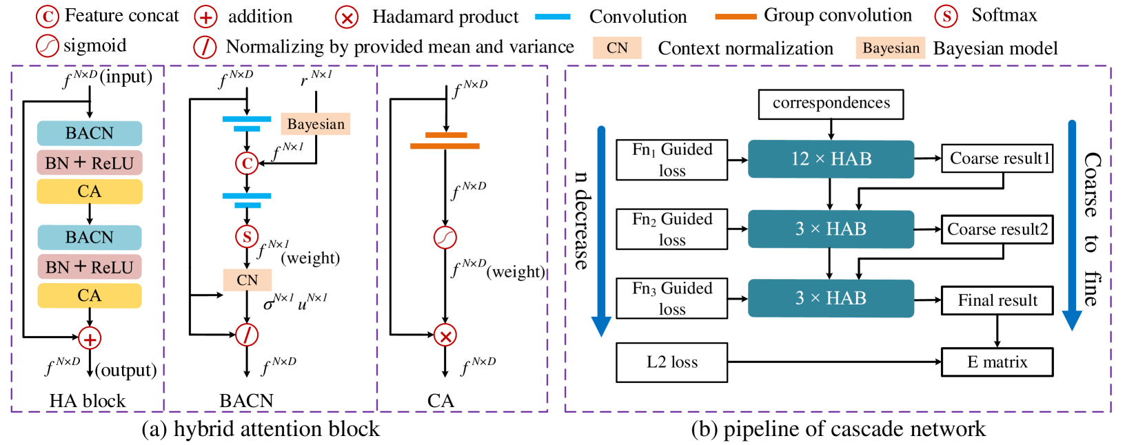
The basic feature extraction block of our network is the proposed hybrid attention block (HAB). As shown in Fig. 2 (a), the input of the HAB is the feature map (output of last layer or data points at layer zero), where is the number of correspondences and is the number of channels. HAB integrates Bayesian attentive context normalization (BACN), batch normalization (BN) (Ioffe and Szegedy 2015), ReLU and Channel-wise Attention (CA) operations in the structure of Res-Net (He et al. 2016). Specifically, BACN is to normalize each correspondence so that the features of correct and incorrect correspondences are distinguishable. BN is adopted to accelerate network convergence and ReLU function is utilized as an activation function. Finally, the CA operation learns the statistical information on the channel to boost the performance of the network.
Bayesian Attentive Context Normalization. We first briefly introduce how our BACN learns distinguishable features for inliers and outliers. In fact, the inliers are under the constraint of an matrix while outliers are not (Hartley and Zisserman 2004). In BACN, a global context is utilized to replace the constraint of matrix to normalize each correspondence. We use statistical information, i.e., the mean and variance of all features, as the global context. Since the global context is expected to fit the distribution of inliers, we use a weighted mean and variance as the global context, so that the outliers can be ignored by the weight vector. Then, we use the context normalization (Moo Yi et al. 2018) operation to encode feature for each correspondence, as follows:
| (14) |
where is the feature of correspondence in -th layer. and are the weighted mean and variance.
The key to BACN is how to better learn the weight vector for computing weighted mean and variance. In the shallow layers of the network, it’s hard to learn appropriate weight vector because the features in these layers are less recognizable. Since Lowe Ratio (Lowe 2004), which is generated during feature matching, is proved useful for determining the confidence of each correspondence being inlier, we expect to use it to make up for the dilemma of weight learning in shallow network. However, the distribution of Lowe Ratio is quite different on different datasets, while independence and identical distribution of features is a very important assumption in neural networks (Bishop 2006). To make better use of Lowe Ratio, we first use the Bayesian Model (Bishop 2006) to convert the it into a probability value. Formally, given a pair of correspondence with Lowe Ratio , we consider as a variable and the joint probability distribution function (PDF) can be modeled as:
| (15) |
where belongs to an inlier, belongs to an outlier, and is the inlier ratio of the putative correspondence set of a specific image pair. Then, the prior probability that the -th correspondence belongs to inlier can be calculated as follows:
| (16) |
Before training, we obtain the PDF of inlier () and outlier () on the training dataset with ground-truth as empirically PDF. Then for each image pair, we estimate the inlier ratio using a curve fitting method (Goshen and Shimshoni 2008). Thus we assign a prior probability to each correspondence by Eq. 16.
After obtaining the prior probability for each correspondence, it will be utilized to participate in the calculation of weight vector. The architecture of weight learning is inspired by Bayesian Model (Bishop 2006). The prior probability is similar to the prior probability of Bayesian Model. Meanwhile, as shown in Fig. 2 (a), the input of BACN is followed with two convolution operation to learn a temporary weight vector, which is similar to the likelihood probability of Bayesian Model. The prior probability and the likelihood probability are fused through a feature concatenate operation to generate a feature which encode the information of posterior probability. After that, the posterior feature is followed by two convolution and a softmax operations to produce weight vector. By incorporating prior information, our network is easier to obtain better classification results.
Channel-wise Attention. The statistics on the channel have been shown to have a significant impact on the network (Hu, Shen, and Sun 2018; Wang et al. 2019). In order to enhance the channel awareness of the network, we introduce channel-wise attention to the HA block. We learn a channel weight vector for each correspondence instead of a weight vector that is shared by all the correspondences to capture complex channel context. When learning the weight vector, group convolution (Cohen and Welling 2016) is used to reduce network computation. Formally, Let be the feature of correspondence in -th layer, then the CA can be expressed as follows:
| (17) |
where is obtained by performing two group convolution operations (Cohen and Welling 2016) and a sigmoid function on the feature as shown in Fig. 2 (a).
Cascade Architecture
Since the proposed Guided Loss can flexibly control the bias on precision and recall by using different Fn-measure as guidance, we can naturally build a cascade network by Guided Loss to progressively refine the performance. Specifically, as shown in Fig. 2 (b), we first use a 12-layer hybrid attention blocks as feature extraction module to extract the feature for each correspondence. Then a coarse result (coarse result1 in Fig. 2 (b)) can be obtained through these features by -measure Guided Loss. Then two refinement modules are followed to perform local optimization to refine the coarse result. Each refinement module is made up of a 3-layer HA Block. Different from feature extraction module, the global context in refinement module is extracted from the coarse result of the previous module instead of all of the correspondences. Besides, in order to gradually optimize the coarse result, the loss function will also progressively bias the precision. The coarse result2 is obtained by -measure Guided Loss, and the final result is obtained by -measure Guided Loss. During training, holds so that the network gradually obtains result with higher precision. Finally, the matrix is computed by performing weighted eight-point or RANSAC algorithm on the final result, and it is supervised by a -.
| YFCC100MSUN3D | COLMAP | |||||||||
|---|---|---|---|---|---|---|---|---|---|---|
| P | R | F1 | mAP | mAP | P | R | F1 | mAP | mAP | |
| CN-Net | 37.23 | 73.21 | 47.08 | 15.12/33.11 | 31.87/43.47 | 27.95 | 65.63 | 39.82 | 11.82/26.89 | 18.44/30.82 |
| PointNet | 27.83 | 47.23 | 32.48 | 12.12/26.31 | 27.85/33.92 | 13.60 | 41.77 | 27.66 | 10.41/25.65 | 17.94/28.76 |
| ACN-Net | 41.09 | 80.96 | 50.68 | 27.91/37.18 | 37.86/47.54 | 30.13 | 76.83 | 38.10 | 23.15/32.51 | 27.32/35.88 |
| NM-Net | 40.66 | 71.66 | 50.74 | 17.70/34.09 | 32.80/42.92 | 31.99 | 54.48 | 38.92 | 20.96/31.72 | 23.08/33.42 |
| -Net | 40.92 | 75.34 | 51.68 | 14.52/32.65 | 30.27/42.16 | 26.88 | 62.91 | 33.26 | 10.90/25.68 | 16.74/29.77 |
| OA-Net | 40.88 | 72.33 | 48.58 | 30.53/37.80 | 39.84/49.87 | 37.41 | 57.74 | 42.88 | 26.82/34.57 | 29.99/37.09 |
| Ours | 53.46 | 70.59 | 59.67 | 31.25/41.90 | 41.52/52.57 | 42.08 | 55.21 | 46.76 | 27.82/36.83 | 30.80/39.26 |


Loss Function. We formulate our objective as a combination of two types of loss functions, including classification and regression loss. The whole loss function is as follows:
| (18) |
is related with the final result in Fig. 2, and and are related with the coarse result1 and coarse result2 in Fig. 2 respectively. For the regression loss , we use geometric - for matrix (Moo Yi et al. 2018) as follows:
| (19) |
where and are the estimated and ground truth matrix, respectively.
Experiments
Experimental Setup
Parameter Settings. The network is trained by Adam optimizer (Kingma and Ba 2015) with a learning rate being and batch size being 16. The iteration times are set to 200k. In Eq. 18, the loss weight is 0 during the first 20k iteration and then 0.1 later. and are set to 0.1 during the whole training. The , and in Fig. 2 are set to 0.3, 0.25 and 0.2 during training, which leads to best relative pose estimation results.
Datasets. We mainly evaluate our method on two benchmark datasets. The first dataset is YFCC100MSUN3D dataset (Moo Yi et al. 2018). Yi et al. choose 5 scenes from the YFCC100M dataset (Thomee et al. 2016) as outdoor scene and 16 scenes from SUN3D dataset (Xiao, Owens, and Torralba 2013) as indoor scene. The ground truth for outdoor and indoor scenes is generated from VSfM (Wu 2013) and KinectFusion (Newcombe et al. 2011). We use their dataset and exact data splits. The second dataset is COLMAP dataset, which is published by Zhao et. al (Zhao et al. 2019a). It contains 16 outdoor scenes. We also use their dataset and exact data splits.
Evaluation Criteria. In the test, we use the trained classification network to get the correspondence classification results, and employ the precision (P), recall (R), F1-measure (F1) (Van Rijsbergen 1974) as the evaluation criteria. Then we perform weighted eight-point (Moo Yi et al. 2018) and RANSAC (Fischler and Bolles 1981) methods as post-processing on the classified correspondence to recover the matrix between the image pair. In order to evaluate the results of the relative pose estimation, we recover the rotation and translation vectors from the estimated matrix and report mAP under , as the metrics respectively (Moo Yi et al. 2018; Zhang et al. 2019).
| module | result | ||||||||||
|---|---|---|---|---|---|---|---|---|---|---|---|
| CN-Net | BACN | CA | ACN | G-Loss | No-cas | cas | P | R | F1 | mAP | mAP |
| ✓ | 37.23 | 73.21 | 47.08 | 15.12/33.11 | 31.87/43.47 | ||||||
| ✓ | ✓ | 43.06 | 79.89 | 52.63 | 26.32/36.14 | 36.41/46.88 | |||||
| ✓ | ✓ | 42.16 | 81.22 | 52.76 | 26.91/36.85 | 37.02/47.48 | |||||
| ✓ | ✓ | ✓ | 44.08 | 81.35 | 53.48 | 27.83/37.99 | 37.82/48.29 | ||||
| ✓ | ✓ | 40.20 | 80.01 | 50.48 | 25.87/35.68 | 35.66/46.04 | |||||
| ✓ | ✓ | ✓ | ✓ | 51.32 | 68.27 | 57.55 | 29.95/39.88 | 39.38/50.02 | |||
| ✓ | ✓ | ✓ | ✓ | ✓ | 52.09 | 68.20 | 57.92 | 30.32/40.18 | 40.25/50.51 | ||
| ✓ | ✓ | ✓ | ✓ | ✓ | 53.46 | 70.59 | 59.67 | 31.25/41.90 | 41.52/52.57 | ||
Comparison to Other Baselines
We compare our network with other state-of-the-art methods, including CN-Net (Moo Yi et al. 2018), PointNet (Qi et al. 2017a), ACN-Net (Sun et al. 2020), NM-Net (Zhao et al. 2019a), -Net (Plötz and Roth 2018) and OA-Net (Zhang et al. 2019) on both YFCC100MSUN3D and COLMAP datasets. All the networks are trained with the same setting. Tab. 4 summarizes the correspondence classification and relative pose estimation results. Our method shows improvement of 15.59% and 6.94% over CN-Net (baseline of our network) in terms of F1-measure on both YFCC100MSUN3D and COLMAP datasets. In terms of pose estimation results, the mAP of our network is also better than CN-Net by more than 10%. Besides, when compared with another network, our method performs best, especially on correspondence classification task, by nearly 5 to 10 % over the current best approach in terms of F1-measure. These experiments demonstrate that the proposed network behaves favorably to the state-of-the-art approaches.
Ablation studies
HA Block. To demonstrate the performance of HA block, we replace the CN Block in the baseline CN-Net (Moo Yi et al. 2018) with the HA block. Both the Bayesian attentive context normalization (BACN) and channel-wise attention (CA) are tested specifically as Tab. 2. As a comparison, we also replace CN Block with ACN Block (Sun et al. 2020) to train the network. Both of the BACN and CA achieve a better result than ACN, and HA block (BACN + CA) achieves an improvement of about 2% over ACN on both correspondence classification and relative pose estimation results.
Guided Loss. We then replace the original loss of CN-Net with our Guided Loss. As shown in Tab. 2, the proposed Guided Loss (CN-Net + BACN + CA + G-Loss) achieves a better performance over the original loss of CN-Net (CN-Net + BACN + CA) on the terms of F1-measure. It shows that the proposed Guided Loss can significantly improve the performance of the classification task. Meanwhile, there is a nearly 2% improvement in the performance of the relative pose task by simply replacing the classification loss without modifying the rest of the network. This is because under the supervision of the proposed Guided Loss, the precision and recall of the classification results are more balanced, which is more conducive to the regression of the matrix.
Cascade vs. No Cascade. In order to show the performance of the proposed cascade architecture, we first deepen the layers of CN-Net from 12 to 18 and test the result as comparison. Meanwhile, we also train the proposed cascade network, which is also a 18-layer network. As shown in Tab. 2, only increasing the number of network layers, the performance of the network is not significantly improved. The performance of cascade network with the same number of layers is significantly better than non-cascaded networks. It implies that using the Guided Loss in a coarse-to-fine cascade manner can significantly improve network performance.
| P | R | F1 | mAP | mAP | |
|---|---|---|---|---|---|
| CE-Loss | 63.21 | 46.33 | 48.67 | 10.12/26.31 | 24.85/39.92 |
| IBCE-Loss | 37.23 | 73.21 | 47.08 | 15.12/33.11 | 31.87/43.47 |
| Focal Loss | 70.67 | 41.44 | 49.67 | 11.32/27.65 | 28.94/41.43 |
| F-Loss | 44.72 | 67.43 | 51.11 | 10.82/28.90 | 26.16/39.27 |
| G-Loss | 50.62 | 66.20 | 56.44 | 18.52/34.83 | 33.41/45.64 |
Guided Loss vs. another loss.
In order to further verify the performance of the proposed Guided Loss, we record the training curves of the weight, precision and recall in Fig. 3. As shown in Fig. 3 (a), in the Guided Loss is dynamically changed, while in IB-CE-Loss is set to fixed value 0.5. As a result, the Guided Loss can achieve a balance between precision and recall, as shown in Fig. 3 (b). Meanwhile, when using F1-measure, which considers precision and recall equally, as the guidance, the gap between precision and recall is always small. And when using F2-measure, which is more bias towards recall, the recall is always higher than precision. It shows that the result of Guided Loss always accords with the guided Fn-measure, which verifies the effect of the guidance.
Meanwhile, we train the CN-Net (Moo Yi et al. 2018) with the different loss functions (Deng et al. 2018; Zhao et al. 2019b; Lin et al. 2017) and precision, recall, F1-measure and mAP under , are reported in Tab. 3. As discussed in Introduction, when using Fn-measure as objective function, some relaxation has to be made and not all of the samples are utilized for back propagation. Therefore, Fn-Loss does not even perform as well as IB-CE-Loss. For the proposed Guided Loss, the network can achieve a better result than the other loss functions. This is because the Guided Loss can maintain the advantages of IB-CE-Loss while achieving a balance between precision and recall.
Conclusion
In this paper, we present a Guided Loss, which shows a new idea of loss designing. In the proposed Guided Loss, the network is expected to optimize the Fn-measure. Instead of directly using Fn-measure as objective function, we propose to use Fn-measure as the guidance and still adopt the form of cross entropy. Thus, we can maintain the advantage of cross entropy loss while optimizing the Fn-measure. In other tasks, the loss function and evaluation criteria may be different from ours, but the idea of using evaluation criteria to adjust objective function can be used to design more loss functions. Besides, a hybrid attention (HA) block, including a Bayesian attentive context normalization and a channel-wise attention, is proposed for better extracting global context. The Guided Loss and HA Block are combined in a cascade network for two-view geometry tasks. Through extensive experiments, we demonstrate that our network can achieve the state-of-the-art performance on benchmark dataset.
Acknowledgements
This work was supported by the National Natural Science Foundation of China under Grant 61772213, Grant 61991412 and Grant 91748204.
Appendix
Proof of Algorithm 1
Theorem. Given two equations as follows:
| (20) |
| (21) |
where and are the partial derivatives of loss () with respect to and , and and are the partial derivatives of Fn-measure () with respect to and . and are the derivatives of and .
Proof. As introduced in the paper, Fn-measure () and loss () are both the dependent variables of X and Y. Specifically, the form of loss is as follows:
| (22) | ||||
where and are the number of positive and negative samples. We compute the average loss terms of , , and samples respectively, denoted as . Then the can be transformed as follows:
| (23) | ||||
Since both the and samples belong to positive class (ground truth is positive), the loss term of each sample are computed by in Eq. 22 , where () is the logit value. In fact, if the logit value of a positive sample (ground truth is positive) is greater than 0.5, then it is a sample. And if the logit value is smaller than 0.5, it is a sample. Obviously, since is a monotone decreasing function, then the loss term of each sample is greater than sample. Thus, the average loss of samples is greater than that of samples, i.e.,
| (24) |
Similarly, the the average loss of samples is greater than that of samples, i. e.,
| (25) |
Then, we can compute the partial derivatives of loss with respect to and from Eq. 23, as follows:
| (26) | ||||
According to the constraints of Eq. 24 and 25, we can obtain the following constraints:
| (27) |
We then perform the same operations on to obtain the constraints of . Specifically, is related with precision () and recall (), and , are both related with , , as follows:
| (28) |
| (29) | ||||
According to the compound derivation formula, we can compute the and as follows:
| (30) | ||||
The , , , all can be computed from Eq. 28 and 29, as follows:
| (31) | ||||
We can easily obtain the following constraints of and from Eq. 30, 31:
| (32) | |||

Meanwhile, since Fn-measure () and loss () are both the dependent variables of X and Y, the differential form of and in Eq. 21 can be expressed as follows:
| (33) | ||||
Thus,
| (34) | ||||
According to the constraints of Eq. 27 and 32, we can further expand Eq. 34 as follows:
| (35) | ||||
If Eq. 20 holds, then,
| (36) |
then,
| (37) | ||||
Additional Experiments
Guided Loss with other baseline networks. We further analyze our Guided Loss by replacing the classification loss functions of other models with Guided Loss. We first train three recent networks, including CN-Net (Moo Yi et al. 2018), ACN-Net (Sun et al. 2019) and NM-Net (Zhao et al. 2019a), with their original classification loss. Then we replace their classification loss with our Guided Loss. The results are reported in Tab. 4. Each network with the supervision of our loss can lead to a result with more balanced precision and recall and a higher F1-measure. As a result, the each network increase the mAP by 1-3% without modifying anything.
| P | R | F1 | mAP | mAP | |
|---|---|---|---|---|---|
| CN-Net | 37.23 | 73.21 | 47.08 | 15.12/33.11 | 31.87/43.47 |
| CN-Net + | 50.62 | 66.20 | 56.44 | 18.52/34.83 | 33.41/45.64 |
| ACN-Net | 40.20 | 80.01 | 50.48 | 25.87/35.68 | 35.66/46.04 |
| ACN-Net + | 49.88 | 66.57 | 57.55 | 27.32/37.13 | 36.98/47.65 |
| NM-Net | 40.66 | 71.66 | 50.74 | 17.70/34.09 | 32.80/42.92 |
| NM-Net + | 46.72 | 65.44 | 55.68 | 19.89/36.79 | 34.32/44.02 |
| P | R | F0.5 | F1 | F1.5 | F2 | F2.5 | |
|---|---|---|---|---|---|---|---|
| G-F0.5 | 64.5 | 51.1 | 60.5 | 56.0 | 53.8 | 52.7 | 52.2 |
| G-F1 | 56.8 | 57.8 | 57.2 | 57.3 | 55.9 | 56.7 | 56.6 |
| G-F1.5 | 48.6 | 64.6 | 50.6 | 54.3 | 58.2 | 59.6 | 60.9 |
| G-F2 | 47.4 | 67.3 | 49.8 | 54.3 | 57.2 | 60.9 | 62.6 |
| G-F2.5 | 43.6 | 69.2 | 46.6 | 52.2 | 57.1 | 60.5 | 63.8 |
| IB-CE | 37.2 | 77.1 | 40.0 | 47.1 | 53.8 | 59.4 | 62.9 |
| CE | 63.2 | 48.3 | 56.7 | 52.1 | 51.1 | 50.7 | 50.5 |
Parameter of Guided Loss. Our Guided Loss is designed to build a perfect negative correlation relationship between cross entropy loss and Fn-measure for better optimizing Fn-measure. To verify that our guidance actually works, we train the CN-Net (Moo Yi et al. 2018) with different Fn-measure Guided Loss, respectively. Meanwhile, we also train the CN-Net with the cross entropy loss (CE-Loss) and Instance Balance cross entropy loss (Deng et al. 2018; Moo Yi et al. 2018) (IB-CE-Loss). The classification result are shown in Tab. 5. We record the precision (P), recall (R), and five Fn-measures (n = 0.5, 1, 1.5, 2, 2.5 respectively) of the classification results on test dataset. As shown in Tab. 5, with the guidance of a specific Fn-measure, our Guided Loss can achieve the best performance on this measurement. It shows the direct guidance of our loss. We can choose the corresponding Fn-measure to guide the loss according to the requirements of precision and recall of different tasks.
References
- Barath and Matas (2018) Barath, D.; and Matas, J. 2018. Graph-cut RANSAC. In Proceedings of the IEEE Conference on Computer Vision and Pattern Recognition, 6733–6741.
- Benhimane and Malis (2004) Benhimane, S.; and Malis, E. 2004. Real-time image-based tracking of planes using efficient second-order minimization. In 2004 IEEE/RSJ International Conference on Intelligent Robots and Systems (IROS)(IEEE Cat. No. 04CH37566), volume 1, 943–948. IEEE.
- Bishop (2006) Bishop, C. M. 2006. Pattern Recognition and Machine Learning (Information Science and Statistics). Berlin, Heidelberg: Springer-Verlag.
- Brahmachari and Sarkar (2009) Brahmachari, A. S.; and Sarkar, S. 2009. BLOGS: Balanced local and global search for non-degenerate two view epipolar geometry. In 2009 IEEE 12th International Conference on Computer Vision, 1685–1692. IEEE.
- Chen et al. (2017) Chen, L.-C.; Papandreou, G.; Kokkinos, I.; Murphy, K.; and Yuille, A. L. 2017. Deeplab: Semantic image segmentation with deep convolutional nets, atrous convolution, and fully connected crfs. IEEE transactions on pattern analysis and machine intelligence 40(4): 834–848.
- Chum and Matas (2005) Chum, O.; and Matas, J. 2005. Matching with PROSAC-progressive sample consensus. In 2005 IEEE Computer Society Conference on Computer Vision and Pattern Recognition (CVPR’05), volume 1, 220–226. IEEE.
- Chum, Matas, and Kittler (2003) Chum, O.; Matas, J.; and Kittler, J. 2003. Locally optimized RANSAC. In Joint Pattern Recognition Symposium, 236–243. Springer.
- Cohen and Welling (2016) Cohen, T.; and Welling, M. 2016. Group equivariant convolutional networks. In International conference on machine learning, 2990–2999.
- Dai et al. (2019) Dai, T.; Cai, J.; Zhang, Y.; Xia, S.-T.; and Zhang, L. 2019. Second-order Attention Network for Single Image Super-Resolution. In Proceedings of the IEEE Conference on Computer Vision and Pattern Recognition, 11065–11074.
- Deng et al. (2018) Deng, D.; Liu, H.; Li, X.; and Cai, D. 2018. Pixellink: Detecting scene text via instance segmentation. In Thirty-Second AAAI Conference on Artificial Intelligence.
- Fischler and Bolles (1981) Fischler, M. A.; and Bolles, R. C. 1981. Random sample consensus: a paradigm for model fitting with applications to image analysis and automated cartography. Communications of the ACM 24(6): 381–395.
- Fragoso et al. (2013) Fragoso, V.; Sen, P.; Rodriguez, S.; and Turk, M. 2013. EVSAC: accelerating hypotheses generation by modeling matching scores with extreme value theory. In Proceedings of the IEEE International Conference on Computer Vision, 2472–2479.
- Goshen and Shimshoni (2008) Goshen, L.; and Shimshoni, I. 2008. Balanced exploration and exploitation model search for efficient epipolar geometry estimation. IEEE Transactions on Pattern Analysis and Machine Intelligence 30(7): 1230–1242.
- Hartley and Zisserman (2004) Hartley, R.; and Zisserman, A. 2004. Multiple View Geometry in Computer Vision. Cambridge University Press, 2 edition.
- He et al. (2016) He, K.; Zhang, X.; Ren, S.; and Sun, J. 2016. Deep residual learning for image recognition. In Proceedings of the IEEE conference on computer vision and pattern recognition, 770–778.
- Hu, Shen, and Sun (2018) Hu, J.; Shen, L.; and Sun, G. 2018. Squeeze-and-excitation networks. In Proceedings of the IEEE conference on computer vision and pattern recognition, 7132–7141.
- Ioffe and Szegedy (2015) Ioffe, S.; and Szegedy, C. 2015. Batch normalization: Accelerating deep network training by reducing internal covariate shift. arXiv preprint arXiv:1502.03167 .
- Kingma and Ba (2015) Kingma, D. P.; and Ba, J. 2015. Adam: A method for stochastic optimization. In Proceedings of the International Conference on Learning Representations.
- Lin et al. (2017) Lin, T.-Y.; Goyal, P.; Girshick, R.; He, K.; and Dollár, P. 2017. Focal loss for dense object detection. In Proceedings of the IEEE international conference on computer vision, 2980–2988.
- Lowe (2004) Lowe, D. G. 2004. Distinctive image features from scale-invariant keypoints. International journal of computer vision 60(2): 91–110.
- Ma et al. (2019) Ma, J.; Jiang, X.; Jiang, J.; Zhao, J.; and Guo, X. 2019. Lmr: Learning a two-class classifier for mismatch removal. IEEE Transactions on Image Processing .
- Mishchuk et al. (2017) Mishchuk, A.; Mishkin, D.; Radenovic, F.; and Matas, J. 2017. Working hard to know your neighbor’s margins: Local descriptor learning loss. In Advances in Neural Information Processing Systems, 4826–4837.
- Moo Yi et al. (2018) Moo Yi, K.; Trulls, E.; Ono, Y.; Lepetit, V.; Salzmann, M.; and Fua, P. 2018. Learning to find good correspondences. In Proceedings of the IEEE Conference on Computer Vision and Pattern Recognition, 2666–2674.
- Newcombe et al. (2011) Newcombe, R. A.; Izadi, S.; Hilliges, O.; Molyneaux, D.; Kim, D.; Davison, A. J.; Kohi, P.; Shotton, J.; Hodges, S.; and Fitzgibbon, A. 2011. KinectFusion: Real-time dense surface mapping and tracking. In 2011 10th IEEE International Symposium on Mixed and Augmented Reality, 127–136. IEEE.
- Plötz and Roth (2018) Plötz, T.; and Roth, S. 2018. Neural Nearest Neighbors Networks. In Advances in Neural Information Processing Systems (NeurIPS).
- Qi et al. (2017a) Qi, C. R.; Su, H.; Mo, K.; and Guibas, L. J. 2017a. Pointnet: Deep learning on point sets for 3d classification and segmentation. In Proceedings of the IEEE Conference on Computer Vision and Pattern Recognition, 652–660.
- Qi et al. (2017b) Qi, C. R.; Yi, L.; Su, H.; and Guibas, L. J. 2017b. Pointnet++: Deep hierarchical feature learning on point sets in a metric space. In Advances in neural information processing systems, 5099–5108.
- Schonberger and Frahm (2016) Schonberger, J. L.; and Frahm, J.-M. 2016. Structure-from-motion revisited. In Proceedings of the IEEE Conference on Computer Vision and Pattern Recognition, 4104–4113.
- Snavely, Seitz, and Szeliski (2006) Snavely, N.; Seitz, S. M.; and Szeliski, R. 2006. Photo tourism: exploring photo collections in 3D. In ACM transactions on graphics (TOG), volume 25, 835–846. ACM.
- Sun et al. (2019) Sun, W.; Jiang, W.; Trulls, E.; Tagliasacchi, A.; and Yi, K. M. 2019. Attentive Context Normalization for Robust Permutation-Equivariant Learning. arXiv preprint arXiv:1907.02545 .
- Sun et al. (2020) Sun, W.; Jiang, W.; Trulls, E.; Tagliasacchi, A.; and Yi, K. M. 2020. ACNe: Attentive Context Normalization for Robust Permutation-Equivariant Learning. In Proceedings of the IEEE/CVF Conference on Computer Vision and Pattern Recognition, 11286–11295.
- Thomee et al. (2016) Thomee, B.; Shamma, D. A.; Friedland, G.; Elizalde, B.; Ni, K.; Poland, D.; Borth, D.; and Li, L.-J. 2016. YFCC100M: The new data in multimedia research. Communications of the ACM 59(2): 64–73.
- Van Rijsbergen (1974) Van Rijsbergen, C. J. 1974. Foundation of evaluation. Journal of documentation 30(4): 365–373.
- Vaswani et al. (2017) Vaswani, A.; Shazeer, N.; Parmar, N.; Uszkoreit, J.; Jones, L.; Gomez, A. N.; Kaiser, Ł.; and Polosukhin, I. 2017. Attention is all you need. In Advances in neural information processing systems, 5998–6008.
- Wang et al. (2019) Wang, L.; Huang, Y.; Hou, Y.; Zhang, S.; and Shan, J. 2019. Graph Attention Convolution for Point Cloud Semantic Segmentation. In Proceedings of the IEEE Conference on Computer Vision and Pattern Recognition, 10296–10305.
- Wang et al. (2018) Wang, X.; Girshick, R.; Gupta, A.; and He, K. 2018. Non-local neural networks. In Proceedings of the IEEE Conference on Computer Vision and Pattern Recognition, 7794–7803.
- Wu (2013) Wu, C. 2013. Towards linear-time incremental structure from motion. In 2013 International Conference on 3D Vision-3DV 2013, 127–134. IEEE.
- Xiao, Owens, and Torralba (2013) Xiao, J.; Owens, A.; and Torralba, A. 2013. SUN3D: A Database of Big Spaces Reconstructed Using SfM and Object Labels 1625–1632.
- Zhang et al. (2019) Zhang, J.; Sun, D.; Luo, Z.; Yao, A.; Zhou, L.; Shen, T.; Chen, Y.; Quan, L.; and Liao, H. 2019. Learning Two-View Correspondences and Geometry Using Order-Aware Network. arXiv preprint arXiv:1908.04964 .
- Zhao et al. (2019a) Zhao, C.; Cao, Z.; Li, C.; Li, X.; and Yang, J. 2019a. NM-Net: Mining Reliable Neighbors for Robust Feature Correspondences. In Proceedings of the IEEE Conference on Computer Vision and Pattern Recognition, 215–224.
- Zhao et al. (2019b) Zhao, K.; Gao, S.; Wang, W.; and Cheng, M.-M. 2019b. Optimizing the f-measure for threshold-free salient object detection. In Proceedings of the IEEE International Conference on Computer Vision, 8849–8857.