Capturing and incorporating expert knowledge into machine learning models for quality prediction in manufacturing
Abstract
Increasing digitalization enables the use of machine learning methods for analyzing and optimizing manufacturing processes. A main application of machine learning is the construction of quality prediction models, which can be used, among other things, for documentation purposes, as assistance systems for process operators, or for adaptive process control. The quality of such machine learning models typically strongly depends on the amount and the quality of data used for training. In manufacturing, the size of available datasets before start of production is often limited. In contrast to data, expert knowledge commonly is available in manufacturing. Therefore, this study introduces a general methodology for building quality prediction models with machine learning methods on small datasets by integrating shape expert knowledge, that is, prior knowledge about the shape of the input-output relationship to be learned. The proposed methodology is applied to a brushing process with data points for predicting the surface roughness as a function of five process variables. As opposed to conventional machine learning methods for small datasets, the proposed methodology produces prediction models that strictly comply with all the expert knowledge specified by the involved process specialists. In particular, the direct involvement of process experts in the training of the models leads to a very clear interpretation and, by extension, to a high acceptance of the models. Another merit of the proposed methodology is that, in contrast to most conventional machine learning methods, it involves no time-consuming and often heuristic hyperparameter tuning or model selection step.
Index terms: Informed machine learning, small datasets, expert knowledge, shape constraints, quality prediction, surface finishing
1 Introduction
The shift from mass production to mass customization and personalization [Hu.2013] requires high standards on production processes. In spite of the high variance between different products and small batch sizes of the products to be manufactured, the product quality in mass customization has to be comparable to the quality of products from established mass production processes. It is therefore essential to keep process ramp-up times low and to achieve the required product quality as directly as possible. This requires a profound and solid understanding of the dependencies between process parameters and quality criteria of the final product, even before the start of production (SOP). Various ways exist to gain this kind of process knowledge: for example, by carrying out experiments, setting up simulations, or exploiting available expert knowledge. In production, expert knowledge in particular plays a central role. This is because complex cause-effect relationships operate between the input-output parameters during machining, and these generally have to be set in a result-oriented manner in a short amount of time without recourse to real-time data sets. Indeed, process ramp-up is still commonly done by process experts purely based on their knowledge. Furthermore, many processes are controlled by experts during production to ensure that consistently high quality is produced.
In the course of digitalization, the acquisition of and the access to data in manufacturing have increased significantly in recent years. Sensors, extended data acquisition by the controllers themselves, and the continuous development of low-cost sensors allow for the acquisition of large amounts of data [Wuest.2016]. Accordingly, more and more data-driven approaches, most notably machine learning methods, are used in manufacturing to describe the dependencies between process parameters and quality parameters [Weichert.2019]. In principle, such data-driven methods are suitable for the rapid generation of quality prediction models in production, but the quality of machine learning models crucially depends on the amount and the information content of the available data. The data can be generated from experiments or from simulations. In general, experiments for process development or improvement are expensive and accordingly the number of experiments to be performed should be kept to a minimum. In this context, design of experiment can be used to obtain maximum information about the process behavior with as few experiments as possible [Montgomery.2017], [Fedorov.2014]. Similarly, the generation of data using realistic simulation models can be expensive as well, because the models must be created, calibrated, and – depending on the process – high computing capacities are required to generate the data. Concluding, the data available in manufacturing before the SOP is typically rather small.
This paper introduces a novel and general methodology to leverage expert knowledge in order to compensate such data sparsities and to arrive at prediction models with good predictive power in spite of small datasets. Specifically, the proposed methodology is dedicated to shape expert knowledge, that is, expert knowledge about the qualitative shape of the input-output relationship to be learned. Simple examples of such shape knowledge are prior monotonicity or prior convexity knowledge, for instance. Additionally, the proposed methodology directly involves process experts in capturing and in incorporating their shape knowledge into the resulting prediction model.
In more detail, the proposed methodology proceeds as follows. In a first step, an initial, purely data-based prediction model is trained. A process expert then inspects selected, particularly informative graphs of this model and specifies in what way these graphs confirm or contradict his shape expectations. In a last step, the thus specified shape expert knowledge is incorporated into a new prediction model which strictly complies with all the imposed shape constraints. In order to compute this new model, the semi-infinite optimization approach to shape-constrained regression is taken, based on the algorithms from [Schmid.2021]. In the following, this approach is referred to as the SIASCOR method for brevity. While a semi-infinite optimization approach has also been pursued in [Kurnatowski.2021], the algorithm used here is superior to the reference-grid algorithm from [Kurnatowski.2021], both from a theoretical and from a practical point of view. Additionally, the paper [Kurnatowski.2021] treats only a single kind of shape constraints, namely monotonicity constraints.
The general methodology is applied to the exemplary process of grinding with brushes. In spite of the small set of available measurement data, the methodology proposed here leads to a high-quality prediction model for the surface roughness of the brushed workpiece.
The paper is organized as follows. Section 2 gives an overview of the related work. In Section 3, the general methodology to capture and incorporate shape expert knowledge is introduced, and its individual steps are explained in detail. Section 4 describes the application example, that is, the brushing process. Section 5 discusses the resulting prediction models applied to the brushing process and compares them to more traditional machine learning models. Section 6 concludes the paper with a summary and an outlook on future research.
2 Some related works
In [Weichert.2019] it is shown that machine learning models used for optimization of production processes are often trained with relatively small datasets. In this context, attempts are often made to represent complex relationships with complex models and small datasets. Also in other domains, such as process engineering [Napoli.2011] or medical applications [Shaikhina.2017], small amounts of data play a role in the use of machine learning methods. Accordingly, there already exist quite some methods to train complex models with small datasets in the literature. These known approaches to sparse-data learning can be categorized as purely data-based methods on the one hand and as expert-knowledge-based methods on the other hand. In the following literature review, expert-knowledge-based approaches that typically require large – or, at least, non-sparse – datasets are not included. In particular, the projection- [Lin.2014, Schmid.2020] and rearrangement-based [Dette.2006, Chernozhukov.2009] approaches to monotonic regression are not reviewed here.
2.1 Purely data-based methods for sparse-data learning in manufacturing
An important method for training machine learning models with small datasets is to generate additional, artificial data. Among these virtual-data methods the mega-trend-diffusion (MTD) technique is particularly common. It was developed by [Li.2007] using flexible manufacturing system scheduling as an example. In [Li.2013] virtual data is generated using a combination of MTD and a plausibility assessment mechanism. In the second step, the generated data is used to train an artificial neural network (ANN) and a support vector regression model with sample data from the manufacturing of liquid-crystal-display (LCD) panels. Using multi-layer ceramic capacitor manufacturing as an example, bootstrapping is used in [Tsai.2008] to generate additional virtual data and then train an ANN. The authors of [Napoli.2011] also use bootstrapping and noise injection to generate virtual data and consequently improve the prediction of an ANN. The methodology is applied to estimate the freezing point of kerosene in a topping unit in chemical engineering. In [Chen.2017] virtual data is generated using particle swarm optimization to improve the prediction quality of an extreme learning machine model.
In addition to the methods for generating virtual data and the use of simple machine learning methods such as linear regression, lasso or ridge regression [Bishop.2006], other machine learning methods from the literature can also be used in the context of small datasets. For example, the multi-model approaches in [Li.2012], [Chang.2015] can be mentioned here. The multi-model approaches are used in the field of LCD panel manufacturing to improve the prediction quality. Another concrete example are the models described in [Torre.2019], which are based on polynomial chaos expansion. These models are also suitable for learning complex relationships in spite of few data points.
2.2 Expert-knowledge-based methods for sparse-data learning in manufacturing
An extensive general survey about integrating prior knowledge in learning systems is given in [Rueden.2021]. The integration of knowledge depends on the source and the representation of the knowledge: for example, algebraic equations or simulation results represent scientific knowledge and can be integrated into the learning algorithm or the training data, respectively.
Apart from this general reference, the recent years brought about various papers on leveraging expert knowledge in specific manufacturing applications. Among other things, these papers are motivated by the fact that production planning becomes more and more difficult for companies due to mass customization. In order to improve the quality of production planning, [Schuh.2019] show that enriching production data with domain knowledge leads to an improvement in the calculation of the transition time with regression trees.
Another broad field of research is knowledge integration via Bayesian networks. In [Zhang.2020] domain knowledge is incorporated using a Bayesian network to predict the energy consumption during injection molding. In [Lokrantz.2018] a machine learning framework is presented for root cause analysis of faults and quality deviations, in which knowledge is integrated via Bayesian networks. Based on synthetically generated manufacturing data, an improvement of the inferences could be shown compared to models without expert knowledge. In [He.2019] Bayesian networks are used to inject expert knowledge about the manufacturing process of a cylinder head to evaluate the functional state of manufacturing on the one hand, and to identify causes of functional defects of the final product on the other hand. Another possibility of root cause analysis using domain-specific knowledge is described by [Rahm.2018]. Here, knowledge is acquired within an assistance system and combined with machine learning methods to support the diagnosis and elimination of faults occurring at packaging machines.
In [Lu.2017], knowledge of the electrochemical micro-machining process is incorporated into the structure of a neural network. It is demonstrated that integrating knowledge achieves better prediction accuracy compared to classical neural networks. Another way to integrate knowledge about the additive manufacturing process into neural networks is based on causal graphs and proposed by [Nagarajan.2019]. This approach leads to a more robust model with better generalization capabilities. In [Ning.2019], a control system for a grinding process is presented in which, among other things, a fuzzy neural network is used to control the surface roughness of the workpiece. Incorporating knowledge into models using fuzzy logic is a well-known and proven method, especially in the field of grinding [Brinksmeier.2006].
3 A methodology to capture and incorporate shape expert knowledge
As has been pointed out in the previous section, there are expert-knowledge-free and expert-knowledge-based methods to cope with small datasets in the training of machine learning models in manufacturing. An obvious advantage of expert-knowledge-based approaches is that they typically yield models with superior predictive power, because they take into account more information than the pure data. Another clear advantage of expert-knowledge-based approaches is that their models tend to enjoy higher acceptance among process experts, because the experts are directly involved in the training of these models.
Therefore, this paper proposes a general methodology to capture and incorporate expert knowledge into the training of a powerful prediction model for certain process output quantities of interest. Specifically, the proposed methodology is dedicated to shape expert knowledge, that is, prior knowledge about the qualitative shape of the considered output quantity as a function
| (3.1) |
of relevant process input parameters . Such shape expert knowledge can come in many forms. An expert might know, for instance, that the considered output quantity is monotonically increasing w.r.t. , concave w.r.t. , and monotonically decreasing and convex w.r.t. .
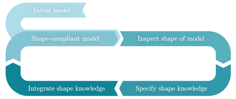
In a nutshell, the proposed methodology to capture and incorporate shape expert knowledge proceeds in the following four steps.
-
1.
Training of an initial purely data-based prediction model
-
2.
Inspection of the initial model by a process expert
-
3.
Specification of shape expert knowledge by the expert
-
4.
Integration of the specified shape expert knowledge into the training of a new prediction model which strictly complies with the imposed shape knowledge.
This new and shape-knowledge-compliant prediction model is computed with the help of the SIASCOR method [Schmid.2021] and it is therefore referred to as the SIASCOR model. After a first run through the steps above, the shape of the SIASCOR model can still be insufficient in some respects, because the shape knowledge specified at the first run might not have been complete, yet. In this case, step two to four can be passed through again, until the expert notices no more shape knowledge violations in the final SIASCOR model. Schematically, this procedure is sketched in Figure 1.
In the remainder of this section, the individual steps of the proposed methodology are explained in detail. The input parameter range on which the models are supposed to make reasonable predictions is always denoted by the symbol . It is further assumed that is a rectangular set, that is,
| (3.2) |
with lower and upper bounds and for the th input parameter . Additionally, the – typically small – set of measurement data available for the relationship (3.1) is always denoted by the symbol
| (3.3) |
3.1 Training of an initial prediction model
In the first step of the methodology, an initial purely data-based model is trained for (3.1), using standard polynomial regression with ridge or lasso regularization [Bishop.2006]. So, the initial model is assumed to be a multivariate polynomial
| (3.4) |
of some degree , where is the vector consisting of all monomials of degree less than or equal to and where is the vector of the corresponding monomial coefficients. In training, these monomial coefficients are tuned such that optimally fits the data and such that, at the same time, the ridge or lasso regularization term is not too large. In other words, one has to solve the simple unconstrained regression problem
| (3.5) |
where and are suitable regularization hyperparameters ( corresponding to lasso and corresponding to ridge regression). As usual, these hyperparameters are chosen such that some cross-validation error becomes minimal.
3.2 Inspection of the initial prediction model
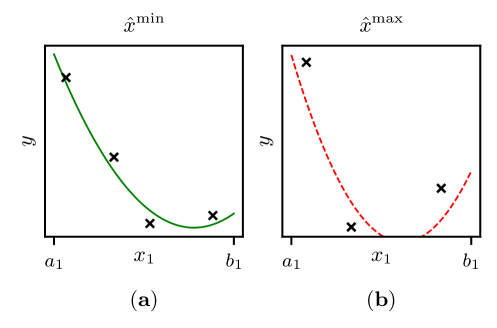
In the second step of the methodology, a process expert inspects the initial model in order to get an overview of its shape. To do so, the expert has to look at - or -dimensional graphs of the initial model. Such - and -dimensional graphs are obtained by keeping all input parameters except one (two) constant to some fixed value(s) of choice and by then considering the model as a function of the one (two) remaining parameter(s). As soon as the number of inputs is larger than two, there are infinitely many of these graphs and it is notoriously difficult for humans to piece them toghether to a clear and coherent picture of the model’s shape [Oesterling.2016]. It is therefore crucial to provide the expert with a small selection of particularly informative graphs, namely graphs with particularly high model confidence and graphs with particularly low model confidence.
A simple method of arriving at such high- and low-fidelity graphs is as follows. Choose those two points , from a given grid
| (3.6) |
in with minimal or maximal accumulated distances from the data points, respectively. In other words,
| (3.7) |
where the gridpoint indices and are defined by
| (3.8) | |||
| (3.9) |
with being the initial model’s prediction at the gridpoint . Starting from the two points and , one then traverses each input dimension range. In this manner, one obtains, for each input dimension , a -dimensional graph of the initial model of particularly high fidelity (namely the function ) and a -dimensional graph of particularly low fidelity (namely the univariate function ). See Figure 2 for exemplary high- and low-fidelity graphs as defined above.
An alternative method of obtaining low- and high-fidelity input parameters and graphs is to use design-of-experiments techniques [Fedorov.2014], but this alternative approach is not pursued here.
After inspecting particularly informative graphs as defined above, the expert can further explore the initial model’s shape by navigating through and investigating arbitrary graphs of the initial model with the help of commercial software or standard slider tools (from Python Dash or PyQt, for instance).