Captured molecules could make a Bose star visible

The ground state wave function may be searched for within the ansatz

where $R$ is a free parameter. The function $\psi(r)$ is the 1s solution of the stationary Schrödinger equation with the potential $V=-\frac{\hbar^{2}}{mRr}$ and energy $E_{0}=-\frac{\hbar^{2}}{2mR^{2}}$.

Making use of the function (8) we find the expectation value of the Hamiltonian (7):

This energy reaches its minimum value

at

The energy of the solution (11) agrees at 90% level with the corresponding numerical result in Ref. [1].¹¹1Numerical solution of the Schrödinger-Poisson equation for the gravitating system on $N$ bosons was first presented in Ref. [1]. The energy of this system in the large $N$ limit was calculated to $E=-0.1626N^{3}G^{2}m^{5}\hbar^{-2}$ which was factor 3 off the correct result $E=-0.05426N^{3}G^{2}m^{5}\hbar^{-2}$ as was pointed out in Ref. [11]. The 10% discrepancy of our solution (11) from the numerical result is still acceptable accuracy for qualitative study of this system considering the simplicity of the trial function (9). For the Gaussian ansatz (16) the error is 5 times smaller.

The root-mean-squared (RMS) radius of this solution is

This quantity characterizes the size of the Bose star. We will use $r_{\mathrm{rms}}$ as the effective boundary of the Bose star in subsequent sections.

As an example, consider a Bose star with mass of Bennu asteroid, $M=7\times 10^{10}$ kg composed of QCD axions with mass $m=10^{-5}$ eV. It consists of $N=4\times 10^{51}$ particles. Its size is

Note that the diameter of the Bennu asteroid is 0.5 km.

The particles in the obtained solution have a distribution of velocities. An important characteristic of this distribution is the root-mean-squared speed, which represents a typical speed of particles in the Bose star,

For the axion star with mass $M=7\times 10^{10}$ considered above, the RMS speed is $v_{\mathrm{rms}}\approx 8\times 10^{-16}c$. Thus, the non-relativistic approximation is justified. However, for solutions with boson mass $m\sim 10^{-5}$ eV and total mass of order the Solar mass, a relativistic treatment is needed.

The simple exponential ansatz (9) for the wave function provides a rather low accuracy for the energy. A better accuracy may be achieved within the Gaussian ansatz [12]

where $R$ is the parameter to be found. Making use of this wave function, we find the expectation value of the Hamiltonian (7):

This energy reaches its minimum value

at

The energy (18) agrees at 98% level with the numerical solution presented in Ref. [1] (see the footnote on page 2). Therefore, we will consider only the Gaussian ansatz in what follows.

The RMS radius calculated with the wave function (16) is

and the RMS speed is

The non-relativistic approximation is applicable for $v_{\mathrm{rms}}\lesssim 0.1c$. Making use of equations (19) and (21), this relation translates into the constraint on the particle number and mass,

The Bose star solution is given by the product of $N$ identical wave functions (16) each describing a particle with mass $m$. They create a gravitational potential $V(r)$ obeying the Poisson equation

where the mass density is

The solution to Eq. (23) reads

On the boundary $r=r_{\mathrm{rms}}$, the gravitational potential is

Thus, the escape velocity on the boundary is

Consider, for example, the QCD axion with mass $m=10^{-5}$ eV and the total mass comparable with the mass of the Earth, $Nm=M_{\oplus}$. The size of this object is about $r_{\mathrm{rms}}\approx 0.4$ m. The corresponding escape velocity at the boundary is $v_{\mathrm{esc}}\approx 0.14c$.

If the DM particle mass is $m=10^{-9}$ eV, the corresponding RMS radius and escape velocity are $r_{\mathrm{rms}}\approx 6.3R_{\oplus}$, $v_{\mathrm{esc}}\approx 4.3$ km/s.

The scalar field $\phi$ is related to the wave function (8) as

Making use of the Gaussian ansatz (16), we find

In the contribution to the energy, this expression should be multiplied by $N(N-1)/2$ which accounts for the pairwise particle interaction. Thus, the total energy of this field configuration reads

This expression reaches its extrema at

The case $\lambda<0$ corresponds to unstable solution because the energy (32) is unbounded from below in this case. However, there is a potential barrier separating energy minimum at $R_{+}$ in Eq. (33) from the collapse area close to $r=0$, with the barrier maximum at $R_{-}$. In the case of small negative $\lambda$, $|\lambda|\ll\pi^{2}\hbar c/[Gm^{2}(N-1)^{2}]$, we obtain minimum of energy

at

and maximum at small $R\propto\lambda$,

In the case of small $\lambda$ this barrier will be sufficiently high to make the decay time of the metastable Bose star exponentially long, making this kind of Bose star potentially observable. This result is similar to the gravitational instability of scalar fields discussed in Ref. [13].

For positive selfinteraction constant, $\lambda>0$, only “+” solution in Eq. (33) is physical. If $\lambda$ is sufficiently small, the leading contribution has the same form as in Eq. (35). For strong selfinteraction, $\frac{2\lambda Gm^{2}(N-1)^{2}}{3\pi^{2}\hbar c}\gg 1$, the parameter $R$ is independent of $N$,

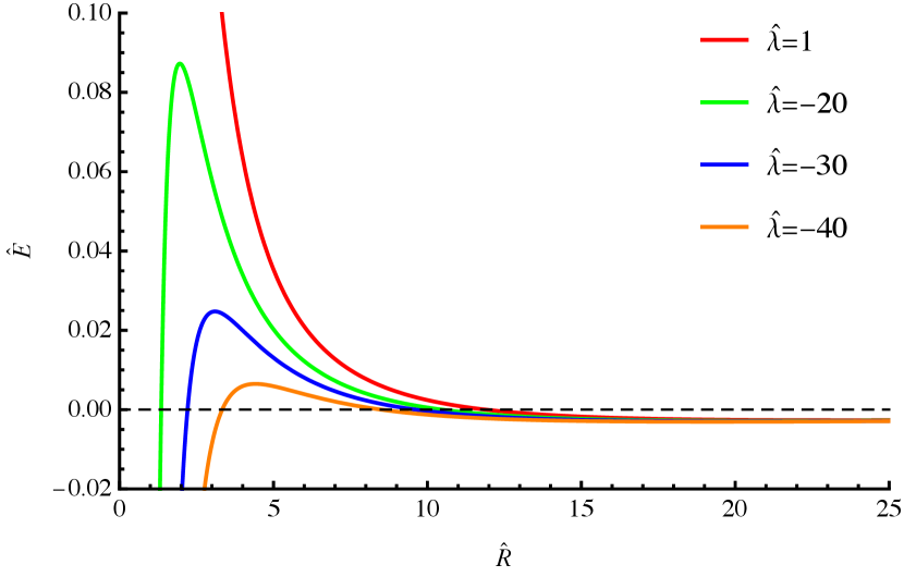
For an illustration of the above results, let us introduce an unitless energy of the solution $\hat{E}=E/E_{0}$, where $E_{0}=mNc^{2}$ is rest energy of the Bose star. Making use of Eqs. (32) this unitless energy may be represented as follows

where we have introduced the following unitless parameters:

For instance, consider a Bose star solution with total mass $M=M_{\oplus}$ composed of particles with mass $m=10^{-5}$ eV. In this case, $\hat{G}\approx 0.2$, and the typical behaviour of the unitless energy (38) is presented in Fig. 1 for various values of $\hat{\lambda}$ ranging from -40 to 1. This function has a shallow minimum near $\hat{R}_{\mathrm{+}}\approx 3\sqrt{\pi}/\hat{G}\approx 24$, and a finite potential barrier for negative $\hat{\lambda}$. For positive $\hat{\lambda}$ this barrier becomes infinitely high.

Note that for the QCD axion, $\phi$, the potential reads $V(\phi)=m^{2}f_{a}^{2}[1-\cos(\phi/f_{a})]=\frac{1}{2}m^{2}\phi^{2}-\frac{m^{2}}{4!f_{a}^{2}}\phi^{4}+\ldots$, where $f_{a}$ is the axion decay constant. The latter is related to the axion mass, $f_{a}/\mbox{TeV}\simeq 6\mbox{\,keV}/m$, and the values $f_{a}\lesssim 10^{9}$ GeV are excluded, see, e.g., [14]. Thus, for the QCD axion, the selfinteraction constant is small and negative,

The full axion potential $V(\phi)$ is, however, non-negative.

In the case of Bose stars, making use of Eq. (29) the condition (44) may be cast in the form

Representing the gas particle mass as $m_{\mathrm{gas}}=Am_{p}$, with $m_{p}$ the proton mass, we find the condition on the atomic number $A$ of gas particles captured near the surface of the Bose star,

The temperature in cold molecular clouds in our Galaxy is typically in the range from 10 to 20 K. Assuming $T=10$ K, we estimate the possibility of capture of gases in the fuzzy dark matter with $m=10^{-22}$ eV and total mass of the object $M=Nm=10^{7}M_{\odot}$:

Thus, this object can accumulate only heavy atoms and molecules, as well as dust particles.

In Fig. 2a, we present plots of mass (and radius) of the Bose star as a function of scalar particle mass $m$ which can capture molecules with atomic mass numbers $A=1$, 10, and 100.

If radius $R$ of Bose star is small, there will be too little matter inside the star and impossible to observe it. However, matter may be captured to distant orbits, but this will require bigger mass $M$ of the star, since the escape velocity will be smaller; for matter at distance $r$, the required star mass is $M(r)=M_{0}R/r$, where $M_{0}$ is the star mass required to capture matter inside.

Cold molecular gas and dust may also be captured by large axion clusters.

If matter capture conditions are fulfilled inside Bose star for all $A$, there will be violation of such conditions outside Bose star at some distance $r$ from the centre. Firstly, this condition will be violated for $A=1$, going further, for higher $A$. Therefore, there will be separation of heavy and light elements outside the Bose star. This is important for Bose star of large mass and small radius.

The results of this subsection qualitatively apply to the case of attractive self-interaction with small negative $\lambda$. In this case the size parameter $R$ receives a small correction (35) which may be neglected in the result (46). The case of strong attractive interaction is not interesting within the present work because it leads to collapse of the boson star to the center and raises the questions of survival of spatially non-compact solutions.

In the case of dominant self-interaction with positive coupling constant $\lambda>0$, the size parameter $R$ is given by Eq. (37). Near the boundary of the Bose star, $r=r_{\mathrm{rms}}$, the repulsive self-interaction energy (32d) becomes comparable with the gravitational attraction one (32b), but it quickly drops with distance by the law $\frac{1}{r^{3}}$. Therefore, we can still use Eqs. (28) and (29), but with the size parameter $R$ defined by Eq. (37). As a result, we find the following expression for the escape velocity,

Making use of the empirical relation (44) and the ideal gas root-mean-squared velocity $v_{\mathrm{rms}}=\sqrt{3k_{B}T/m_{\mathrm{gas}}}$, we find the condition of the capture of gas particles with mass $m_{\mathrm{gas}}$:

This relation may be rewritten for the atomic number $A\equiv m_{\mathrm{gas}}/m_{p}$,

Note that in contrast with Eq. (46) this relation has different dependence on the total Bose star mass $M$.

In Fig. 2b we present plots of mass of the Bose star as a function of scalar particle mass $m$ which can capture molecules with atomic mass numbers $A=1$, 10 and 100 in the case of repulsive scalar particle self-interaction with the coupling $\lambda=10^{-53}$.

References

- Ruffini and Bonazzola [1969] R. Ruffini and S. Bonazzola, Phys. Rev. 187, 1767 (1969).
- Tkachev [1986] I. Tkachev, Sov. Astron. Lett. 12, 305–308 (1986).
- Levkov et al. [2017] D. G. Levkov, A. G. Panin, and I. I. Tkachev, Phys. Rev. Lett. 118, 011301 (2017).
- Marsh [2016] D. J. E. Marsh, Physics Reports 643, 1 (2016).
- Eggemeier and Niemeyer [2019] B. Eggemeier and J. C. Niemeyer, Phys. Rev. D 100, 063528 (2019).
- Chen et al. [2021] J. Chen, X. Du, E. W. Lentz, D. J. E. Marsh, and J. C. Niemeyer, Phys. Rev. D 104, 083022 (2021), arXiv:2011.01333 [astro-ph.CO] .
- Gorghetto et al. [2024] M. Gorghetto, E. Hardy, and G. Villadoro, More Axion Stars from Strings (2024), arXiv:2405.19389 [hep-ph] .
- Schive et al. [2014] H.-Y. Schive, T. Chiueh, and T. Broadhurst, Nature Phys. 10, 496 (2014), arXiv:1406.6586 [astro-ph.GA] .
- Veltmaat and Niemeyer [2016] J. Veltmaat and J. C. Niemeyer, Phys. Rev. D 94, 123523 (2016), arXiv:1608.00802 [astro-ph.CO] .
- Visinelli et al. [2018] L. Visinelli, S. Baum, J. Redondo, K. Freese, and F. Wilczek, Physics Letters B 777, 64 (2018).
- Membrado et al. [1989] M. Membrado, A. F. Pacheco, and J. Sañudo, Phys. Rev. A 39, 4207 (1989).
- Chavanis [2011] P.-H. Chavanis, Phys. Rev. D 84, 043531 (2011).
- Khlopov et al. [1985] M. Y. Khlopov, B. A. Malomed, and Y. B. Zeldovich, Mon. Not. Roy. Astron. Soc. 215, 575 (1985).
- Sikivie [2024] P. Sikivie, Nucl. Phys. B 1003, 116500 (2024).