Capability Augmentation for Heterogeneous Dynamic Teaming
with Temporal Logic Tasks
Abstract
This paper considers how heterogeneous multi-agent teams can leverage their different capabilities to mutually improve individual agent performance. We present Capability-Augmenting Tasks (CATs), which encode how agents can augment their capabilities based on interactions with other teammates. Our framework integrates CAT into the semantics of Metric Temporal Logic (MTL), which defines individual spatio-temporal tasks for all agents. A centralized Mixed-Integer Program (MIP) is used to synthesize trajectories for all agents. We compare the expressivity of our approach to a baseline of Capability Temporal Logic Plus (CaTL+). Case studies demonstrate that our approach allows for simpler specifications and improves individual performance when agents leverage the capabilities of their teammates.
I Introduction
In this paper, we consider a team of agents with varying capabilities and individual tasks, i.e. each agent has a task that it alone is responsible for completing. We focus on tasks where agents need to traverse an environment to reach regions where they can fulfill service requests while avoiding dangerous regions. In certain cases, we identify that agents may be able to fulfill requests without being in the proper regions and stay safe in dangerous regions if they are accompanied by agents with complementary capabilities.
For example, consider a ground agent that must stay dry but travel through regions with water if it is carried by an aerial agent. Collaboration between these agents could improve their ability to satisfy their tasks. We call this capability-augmenting collaboration.
In this work, we focus on generating high-level motion plans for a team of agents using capability-augmenting collaboration. We assign the agents spatio-temporal tasks that include servicing requests and avoiding danger using a rich specification language and formulate a planner to generate trajectories for the team of agents. Our goal is to maximize the number of agents that complete their tasks and minimize the distance they travel.
Previous works explore agents satisfying tasks in heterogeneous teams [1, 2, 3, 4, 5]. [1] demonstrates improvements in rescues made in search and rescue settings, [2] shows improvements in coverage of domains where regions require different mobility capabilities, and [3] shows improvements resilience in networked systems. These works provide ample justification for further exploitation of heterogeneity in multi-agent systems. Works such as [6, 7, 8, 9, 10, 11, 12, 13] provide a foundation for how various tasks are allocated and completed using a team of robots based on agent capabilities. The authors of [6] assign tasks based on system resilience and energy efficiency use, and [7] and [8] assign tasks based on cooperation constraints between agents. In this paper, we build on these works by formalizing a method for agents with tasks that are already allocated to better leverage their heterogeneity through capability-augmenting collaboration.
We use Metric Temporal Logic (MTL) [14][15] to formalize the spatio-temporal tasks for the agents. MTL is a rich specification language that allows us to assign tasks based on concrete time intervals. Works such as [16, 17, 18, 19] offer task allocation and planning formulations for heterogeneous teams using temporal logic specifications. For instance, the authors of [16] defined specifications with Capability Temporal Logic plus (CATL+) in a disaster response scenario, and [17] defined a construction task for modular and reconfigurable robots using MTL. It is often difficult or intractable to specify that tasks can be satisfied using capability-augmenting collaboration in these formulations. We provide a detailed comparison between previous methods and ours in Section IV to demonstrate our method’s benefits.
In this paper we build on the tools designed for specification and verification of behaviors of teams of robots, such as [18, 20, 21, 17, 22, 23, 24, 25, 26, 27], by introducing a formalization for capability-augmenting collaboration using MTL. We use a special case of MTL in which we introduce Capability-Augmenting Tasks (CATs) to simplify the encoding of capability-augmenting collaboration. Specifically, the contributions of this work are as follows:
-
1.
We formalize a planning problem for a team of heterogeneous agents using capability-augmenting collaboration in MTL.
-
2.
We formulate a centralized Mixed Integer Program (MIP) to generate trajectories for the agents.
-
3.
We demonstrate the benefit of capability-augmenting collaboration in satisfying individual tasks in comparison to systems where it is not used.
We formalize the problem of agents utilizing capability-augmenting collaboration and motivate the need to generate group trajectories in Sec. II. We present an approach for generating motion plans that satisfy as many individual tasks as possible while minimizing the distance the agents travel using an MIP in Sec. III. In Sec. IV, we compare the types of collaboration that our formulation can capture to previous work. Finally, we use a case study to demonstrate the benefits of using capability-augmenting collaboration in Sec. V.
II Problem Statement
In this section, we formalize the planning problem for a team of agents using capability-augmenting collaboration to satisfy individual tasks. First, we provide a model for the agents and environment. We then use this model to define individual tasks for the agents using metric temporal logic. We then introduce our method for encoding capability-augmenting collaboration using CATs. Finally, we use our model of the agents and environment, along with the MTL tasks, to formalize a planning problem that we can approach solving in the next section.
To create this formalization, we introduce some basic notation. In this work, we use to describe the set of non-negative real numbers, and denotes the set of non-negative integers. denotes the cardinality of a set. denotes the L-1 norm. Let denote the power set of set .
II-A System Model
In this section, we formalize a model for the agent and environment. We consider a group of heterogeneous agents operating in a partitioned 2D shared environment. In each region, there can either be a service request that an agent can satisfy by visiting that region, an indication that the region should be avoided, or neither. Formally, we define the environment as a tuple , where is the set of nodes (vertices) corresponding to environment regions and is the set of directed edges such that iff an agent can transition from node to node (this includes self-transitions). The environment we consider is a grid such that all transitions that are not self-transition are the same distance. For , let be the set of nodes that are adjacent to node , i.e., . Let be a set of labels that report the the service requests and indications of danger of the environment, and be a mapping that matches each node to a set of labels. Agents are asked to visit and avoid the features of the environment by referencing if it is in a node with a corresponding label.
We assume that the agents travel between nodes using existing edges. As they travel, they incur costs based on the number of transitions they take that are not self-transitions. The agents are synchronized using a central clock. At every time step the agents either transition to a new node or make a self-transition and stay in place. These transitions always take a single time step. Agents are indexed from a finite set , where is the total number of agents in the environment.
We define an individual agent as a tuple , where is the set of capabilities of agent , . The capabilities of each agent determine how they collaborate with other agents (detailed in Sec. II-B and Sec. II-C). Let be the total set of capabilities held by all the agents in the system, i.e., . We define as the set of indices of agents with a specific capability where , i.e. . Let be the node occupied by agent at time , and be the agent’s initial node. In this paper, we only consider the high-level motion plan, i.e., the transitions of robots between nodes. We assume any number of agents can be in the same node and take the same transitions simultaneously without worry of collision. The inter-agent collision can be avoided by using a lower-level controller tracking the high-level motion plan, which will be considered in future work. We define a group trajectory as the sequence of nodes every agent visits where and is the planning horizon (defined in Sec. II-D).
II-B MTL Specifications
Next, we define our language for specifying tasks for the agents. In this paper, we use MTL [14][15] to formally define an individual specification for each agent. We define the individual MTL specification for an agent over its trace. The trace of agent is defined as , where is the observation of agent at time step , defined as
Here, is the number of agents with capability in the same node with agent at time step excluding agent :
where is a binary indicator function that returns if a statement is true and otherwise. The reason we include is so we can evaluate tasks using capability-augmenting collaboration. The syntax of the MTL we use in this paper is defined as follows:
| (1) |
Here, are time bounds with . is the temporal operator eventually, and requires that has to be true at some point in the time interval . is the temporal operator always, and requires that must be true at all points in the time interval . is the temporal operator until, and requires that is true at some point in and is always true before that. , , and are the negation, conjunction, and disjunction Boolean operators, respectively. AP is an atomic proposition. We will formally encode capability-augmenting collaboration into the atomic propositions in Section II-C. We use to denote that the trace of agent satisfies the MTL formula at time . The time horizon of a formula , denoted as , is the smallest time point in the future for which the observation is required to determine the satisfaction of the formula. Formal definitions of the semantics, as well as the time horizon can be found in [14] and [15].
II-C Capability-Augmenting Task
In this subsection, we define a specific kind of atomic proposition called CATs that we use to formalize and encode capability-augmenting collaboration into MTL.
Definition 1 (Syntax of CATs).
The syntax of a CAT is defined as:
| (2) |
where is a label, are two capabilities, are two non-negative integers.
Intuitively, an agent can satisfy the CAT (2) at time in two ways. The first is to reach a node labeled by a specified , i.e., . In cases when agent cannot reach a node with label , the second way that the agent may be able to satisfy the CAT is that there are at least agents with a compatible capability and less than agents with capability in the agent’s node excluding itself. We refer to as an augmenting capability and as an availability-limiting capability. In other words, if the required number of agents with an augmenting capability are present and available in an agent’s node, then the agent can satisfy the CAT with their assistance without being in a node with the required label . The agents with the augmenting capability are unavailable if and only if there are no less than agents with the availability-limiting capability in the agent’s node excluding itself because we assume that the agents with the augmenting capability may be assisting other agents. We make this conservative assumption to ensure that generating trajectories based on CATs is tractable. We will address relaxing this assumption in future work. The second way to satisfy a CAT, i.e., satisfying it via collaboration, is referred to as capability-augmenting collaboration. The satisfaction of a CAT, referred to as the qualitative semantics, is formulated in the following definition.
Definition 2 (Qualitative Semantics of CAT).
The trace of agent satisfies a at time , i.e., , if and only if:
| (3) |
There are two special cases for a CAT. First, if , which means that agents with capability are always available to collaborate, we remove from the CAT for simplicity, i.e., the CAT is denoted as . Second, if , which means that agents with capability can never collaborate with agent , we remove from the CAT and turn it into for simplicity. In both cases, the semantics (3) can be evaluated without the omitted components.
II-D Problem Formulation
We assign an MTL specification defined over to each agent . We define to quantify the satisfaction of , where maps a trace , an MTL formula , and time step to either or depending on satisfaction. It is defined formally as follows:
| (6) |
This metric does not report the degree of satisfaction as a robustness metric would. Rather, it numerically captures Boolean satisfaction for individual agents. We determine the planning horizon from the individual specifications as . We evaluate the performance of agent using and an individual motion cost. The motion cost is the number of transitions, excluding self-transitions, an agent takes and is formulated as:
| (7) | ||||
We define individual agent performance as:
| (8) |
where is a large enough positive number to prioritize the satisfaction of . Note that we use the nodes that makeup to solve for the sequence of observations , meaning that and are enough to evaluate . should be larger than the largest possible value of an individual cost . is an aggregate metric used to evaluate both task satisfaction and accumulated cost.
Our objective is to find an optimal group trajectory , that utilizes the heterogeneous capabilities of the agents to maximize the agent performance and abide by all motion constraints. We solve for optimal trajectories as follows :
| (9) | ||||
We maximize agent performance rather than constraining the system to satisfy all individual specifications. We do so to allow as many agents as possible to satisfy their specifications when not all specifications are feasible.
Remark 1.
For simplicity, we assume the collaboration between agents does not affect the dynamics of the agents which are represented by the constraints in (9). The relaxation of this assumption will be investigated in future work.
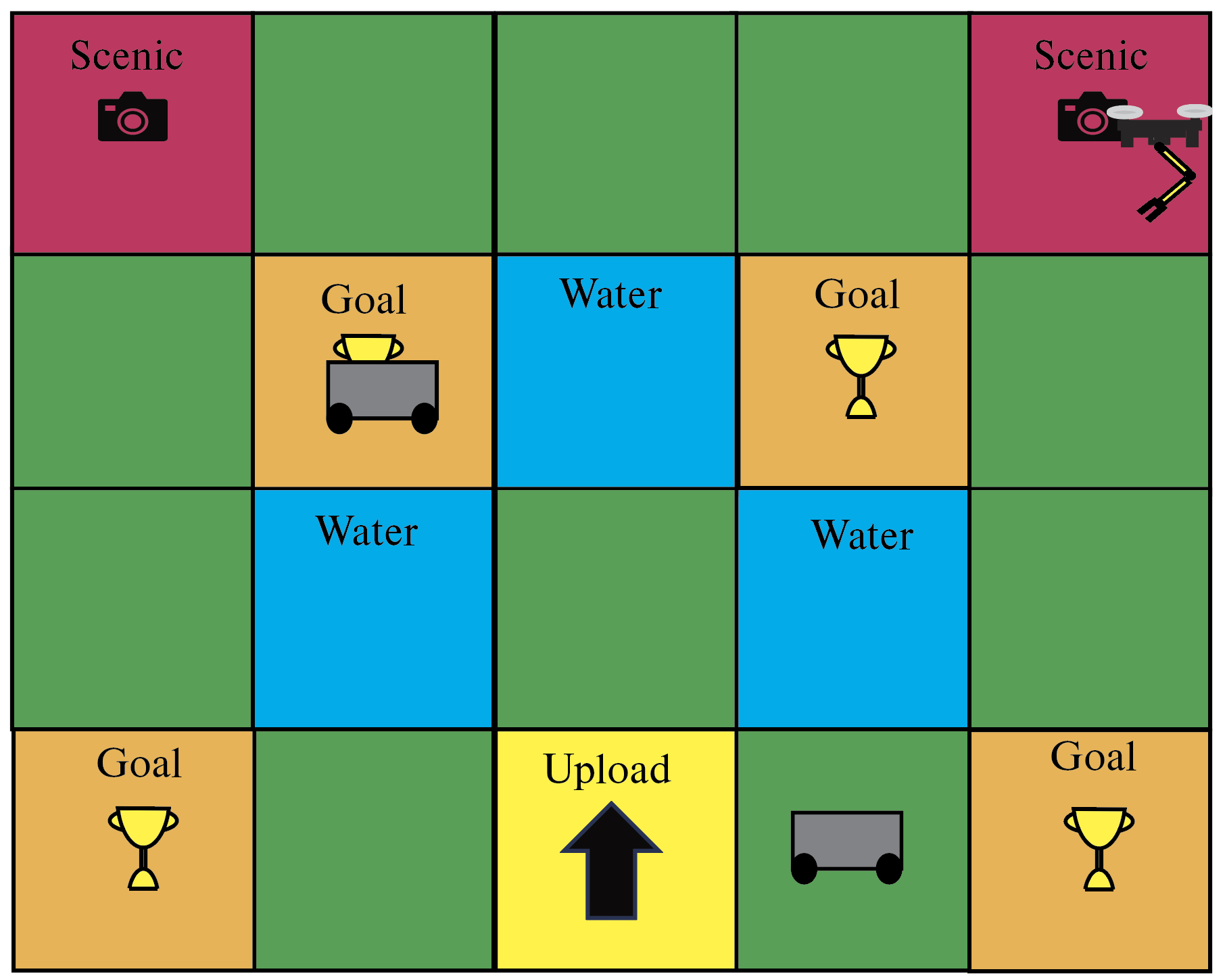
Example: Consider a system composed of three agents () with one aerial and two ground robots (see Fig. 1). The aerial robot must reach a node with the label “Scenic” to take a picture and upload it to a database at a node with the label “Upload”. The ground robots must reach a region with the label “Goal” at some point and never touch “Water”. The ground robot can enter the “Water” regions if it is carried by an aerial agent. The ground robots have a wireless connection to the database that the aerial agent can use to upload its picture when they are together, independently of whether they are in a node with the label “Upload”. The aerial robot can carry one ground robot at a time. Agents plan their trajectories using a central computer, but cannot use it to send or receive images.
We assume that if an agent is in a node where it can perform actions such as taking and uploading pictures, either on its own or in a collaborating way, it does so automatically. All actions happen instantaneously.
The aerial robot has capability . The ground agents have capabilities . As shown in Fig. 1, the environment has labels .
We encode that aerial agent can carry the ground agent over water with a CAT defined over the ground robot. Here, with a slight abuse of notation, we use to denote a label that is assigned to all nodes that are not labeled by , i.e., . This CAT allows the aerial agent to assist the ground robot over water if there are no other ground robots in the same node. The CAT defined over the aerial robot that encodes the aerial agent’s ability to upload pictures using a ground robot is . These CATs provide a succinct encoding that captures capability-augmenting collaboration.
The aerial agent’s specification is to take a picture at “Scenic” in the first 6 time-steps and then upload it within 4 time-steps. The ground agents’ specification is to visit “Goal” in the first 10 time-steps and always avoid “Water” unless carried by an aerial agent. These specifications are encoded as follows:
| (10) |
| (11) |
In this section, we defined capability-augmenting collaboration as a method for agents to utilize each other’s capabilities to satisfy individual specifications. In the next section, we synthesize a Mixed Integer Program to find optimal group trajectories for the agents.
III Approach
III-A Overview
In the previous section, we formulated the problem of synthesizing a group trajectory that satisfies individual MTL specifications using capability-augmenting collaboration as an optimization problem (9). In this section, we detail our approach for solving (9) using a Mixed Integer Program (MIP). To do this, we first need to encode the group trajectories as decision variables and ensure that their motion is constrained as seen in (9). Next, we need to generate variables that allow us to determine the satisfaction of the CATs. Finally, we need to use these variables to solve (9).
III-B Mixed Integer Program Formulation
In this subsection, we define a Mixed Integer Program (MIP) that finds a group trajectory for the agents. The discrete environment and binary and integer elements of the CAT encoding make using an MIP necessary for generating optimal group trajectories.
To begin with, we formulate MIP motion constraints for the individual agents. We define binary decision variables for motion as . If then, agent moves from node to node at time . Otherwise, a different transition is taken. This means that if , then and is and element of the group trajectory . The motion constraints for the trajectory generated at time-step are as follows:
| (12) | |||
| (13) | |||
| (14) |
Constraint (12) encodes an initial node for the agent using the MIP variables. Constraint (13) enforces that an agent may only take one transition at a time. Constraint (14) enforces that agents must either stay in place or move to an adjacent node. These three constraints combined are equivalent to the motion constraint in (9).
We determine for each agent at each time step , i.e. which nodes are included in , as follows where retrieves the index of a node :
| (15) |
To evaluate (9), we need to evaluate and in terms of our MIP variables. Evaluating these allows us to solve (9) through solving (8). To find , we start by encoding the evaluation of CATs into MIP variables. For an individual CAT, we need to retrieve the agents in and that are in the same node as agent using (16). We assign each node a unique index where is the total number of nodes, i.e. . Let represent a binary variable that indicates if agent is in the same node as agent at time step . We determine for agents with capabilities and as follows:
| (16) | |||
Finally, we retrieve the number of agents with capability and in the same node as agent as follows:
| (17) | |||
Next, we define binary variables for the components of the CAT. Let be a binary variable that is if there are at least agents with capability in the same node as agent at time otherwise it is . Let be a binary variable that is if less than agents with capability are in the same node as agent at time otherwise it is . We determine the value of these variables as follows:
| (18) | ||||
Let be a binary variable that is if agent is in a region with label and otherwise. Let be the set of nodes with label , i.e. . We determine the value of as follows:
| (19) |
To quantify the satisfaction of tasks , we use . We find as a function of our decision variables as follows:
| (20) | ||||
We can calculate the individual costs, , using the binary variables as follows:
| (21) |
Note that this returns the same value as (7). The constraints in (III-B)-(17) provide us with infrastructure to determine the satisfaction of individual CATs. We use (III-B)-(19) to evaluate the satisfaction of tasks. Using (20) and (21) we can evaluate agent performance as defined in (8). Finally, (12)-(14) provide the motion constraints found in (9). This accounts for all the pieces required to solve for an optimal group trajectory as defined in (9).
III-C Algorithm
The algorithm that formalizes a procedure for generating group trajectories for a team of heterogeneous agents is given in Algorithm 1
IV Comparison with Existing Formulations
In this section, we compare our ability to capture collaboration between agents to previous formulations. We consider the formulations in [16, 18, 19, 17].
We begin with Capability Temporal Logic Plus (CaTL+) as it is a very rich specification language for heterogeneous teams of agents. We consider a disaster response scenario similar to the case study in [16]. This example has a set of six agents in a 3x3 grid. Two agents are aerial and four are ground. The agents must pick up and deliver medical supplies to villages affected by an earthquake. The agents initialize across a river from the villages. There is a bridge over the river that must be inspected by an aerial agent before the ground agents can use it. Only two ground robots can use the bridge at a time. In [16], the scenario is designed to show the ability to express the need to inspect the bridge before the ground agents use it, a limit on the number of ground agents on the bridge at a time, and a timed delivery task.
In this case, we consider an environment with labels . The aerial agents have indices and and the ground agents have indices . The aerial agents have capabilities . The ground agents have capabilities . This is depicted in Figure 2.
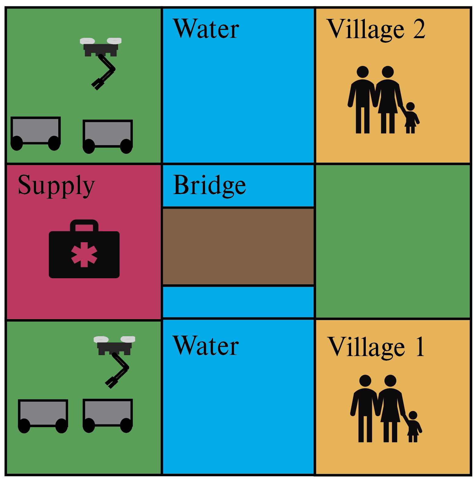
In contrast to CaTL+ which creates a single global specification that is assigned to all agents, we specify a task for each agent. The first aerial agent’s specification is to visit “Village 1” in the first 10 time-steps and not reach “Village 1” until it acquires supplies at “Supply”. The other aerial agent has roughly the same specification except it must visit “Village 2”. The first two ground agents’ specifications are to visit “Village 1” within the first ten time-steps, not to reach “Village 1” until it acquires supplies at “Supply”, never to visit “Water”, and to not visit the bridge at the same time as two other agents with capability “Wheels”. The other two ground agents have roughly the same specifications except the agents must visit “Village 2” instead of “Village 1”. In this case, the CAT encodes the constraint on the maximum number of ground agents on the bridge. Note that we can not capture the constraint that an inspection agent must reach the bridge before the ground agents. This is a constraint that can be captured by CaTL+ by specifying that agents with the capability “wheels” do not visit “Bridge” until it is visited by an agent with the capability “inspection”. We cannot capture this because our formulation is focused on collaboration when agents are in the same node. We show our encoding using CATs for the aerial and ground agents respectively as follows:
| (22) | ||||
| (23) | ||||
However, if we allow the aerial agents to carry one ground agent over “Water” at a time, then this cannot be easily expressed in CaTL+ but can be with our formulation. CaTL+ can specify that multiple agents visit a node labeled “Water”, but directly specify that they meet in the same node. To specify this, we need to specify that they can meet in every state marked “Water” explicitly. This quickly becomes intractable. In our formulation, the ground agents’ tasks become
| (24) | ||||
This shows a clear example of the differences in expressivity between the two formulations. The specifications given by Capability Temporal Logic (CaTL) [18] is a subset of CaTL+. This means that any difficulties experienced in specifying how agents collaborate in CaTL+ are also experienced in CaTL. In CaTL a specified number of agents with a specified capability must visit nodes with a specific atomic proposition (which are similar to labels in our formulation) simultaneously and stay there for a specified amount of time. This makes specifying that agents can satisfy a task without visiting regions with a specific label very difficult.
A similar problem arises in [19] and [17] where tasks focus on agents with a specified capability to spend a certain amount of time in regions with a specific label or proposition. This, again, makes it difficult to specify how agents can satisfy tasks without reaching nodes with a specific label or proposition. However, these formulations all consider global tasks, meaning it is possible to specify constraints such as the inspection in the example, where one agent must visit a node before a different agent.
Our formulation provides the tools to specifically capture capability-augmenting collaboration, which is difficult to express in previous formulations. Next, we show the benefit of this collaboration using a characteristic case study.
V Case Study
In this section, we use a characteristic case study to demonstrate the effectiveness of the methods defined in the previous sections. We show that the use of CATs improves the individual agent performance of agents at satisfying temporal logic specifications. All simulations were run on a computer with 12 i7-8700K CPUs @ 3.70GHz and 15.5 GB of RAM. We used Gurobi as our solver.
V-A Case Study, Aerial and Ground System
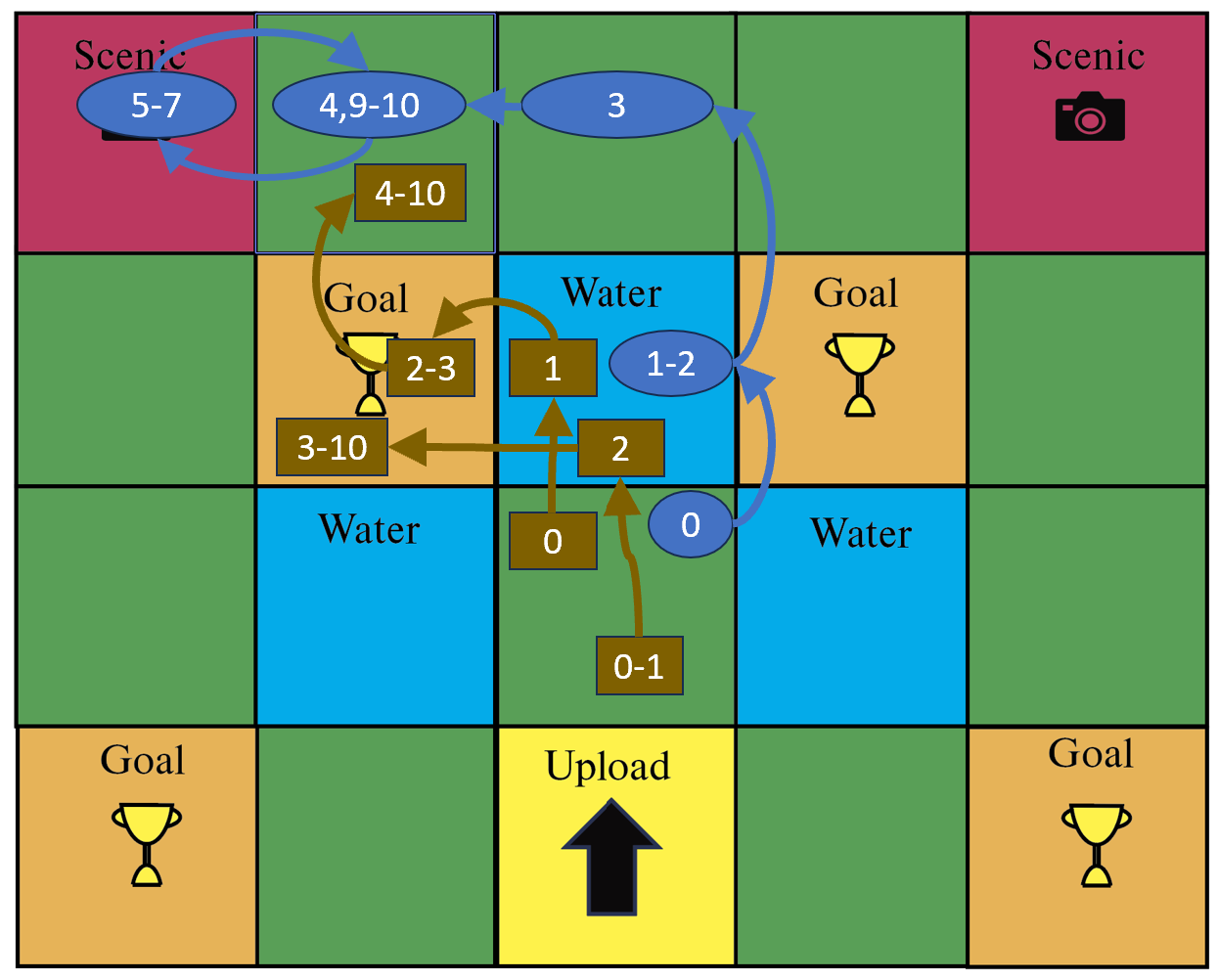
In our case study, we focus on the system with one aerial and two ground agents that we used as an example in the Problem Statement.We use this case study to demonstrate the benefit of using our encoding for capability-augmenting collaboration. Each agent starts in the same node near the environment’s center. The aerial agent has an index of and the ground robots have indices of and .
In this case study, we use an value of when solving (9). The initial node for each agent is the third row and third column of the environment shown in Figure 1. For the three-agent case, we found a solution to this problem in an average of for thirty trials. Each agent completed its task in every trial The average movement for all agents across all trials was transitions. This means that the average individual agent performance was . An example solution is shown in Figure 3. A solver not using CATs, i.e. task satisfaction is solely determined by the labels of the agents’ nodes, could only find solutions for two of the three agents. The motion cost of meaning the average individual agent performance was . The average runtime for the solver not using CATs was . This shows a clear improvement in agent performance when using CATs in this case. However, the runtime using CATs was higher.
Additionally, we increased the number of agents to 5 with 2 aerial agents and 3 ground agents. For this case, we experienced an average runtime of over thirty trials. Once again each agent finished its task in every trial when using CATs. We experience an average motion of transitions for each agent across all trials. This means that the average agent performance was . For the solver not using CATs, only three of the five agents satisfied their tasks and the average motion cost was . This means the average individual agent performance was . We experienced improvements in agent performance with the increased number of agents when using CATs.
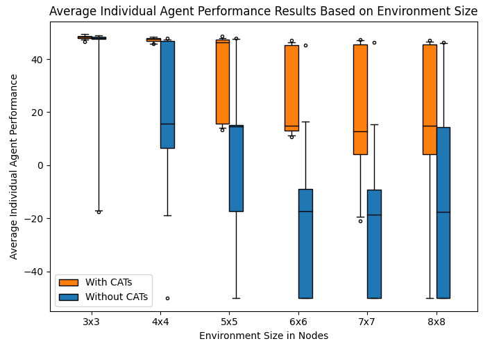
To further investigate the performance of our formulation, we use the tasks given in (10) and (11) and randomize our environment. We generate increasingly large environments to show the effects of CATs as the environment increases in size. We compare this to a system that does not use capability-augmenting collaboration when solving for a trajectory. The results for agent performance are shown in Figure 4. This figure shows the individual agent performance metric defined in (8). These results demonstrate that the use of CATs consistently results in improved individual agent performance. As the environment becomes larger, the desirable nodes (“Scenic”, “Upload”, and “Goal”) become more spread out, making tasks more difficult to satisfy. The use of capability-augmenting collaboration improved the ability of agents to satisfy their tasks in these trials by allowing them to use each other’s capabilities when the desirable nodes are harder to reach.
VI Conclusion
In this paper, we defined a method to encode capability-augmenting collaboration between agents into the language of MTL by introducing CATs. We formulated a mixed integer program to solve problems using CATs. We demonstrated the capabilities of this encoding to find trajectories using case studies.
In this case, we used CATs in individual tasks to show how heterogeneous agents could leverage each other’s capabilities to improve their agent performance. Future work may include creating a global specification formulation that allows individual agents to improve their agent performance using CATs. Additionally, we focus on the problem of generating high-level trajectories for the agents. Future work may focus on creating low-level controllers for agents that utilize these high-level trajectories.
References
- [1] S. S. O V, R. Parasuraman, and R. Pidaparti, “Impact of heterogeneity in multi-robot systems on collective behaviors studied using a search and rescue problem,” in 2020 IEEE International Symposium on Safety, Security, and Rescue Robotics (SSRR), pp. 290–297, 2020.
- [2] S. Kim and M. Egerstedt, “Heterogeneous coverage control with mobility-based operating regions,” in 2022 American Control Conference (ACC), pp. 2148–2153, 2022.
- [3] R. K. Ramachandran, J. A. Preiss, and G. S. Sukhatme, “Resilience by reconfiguration: Exploiting heterogeneity in robot teams,” in 2019 IEEE/RSJ International Conference on Intelligent Robots and Systems (IROS), pp. 6518–6525, 2019.
- [4] P. Twu, Y. Mostofi, and M. Egerstedt, “A measure of heterogeneity in multi-agent systems,” in 2014 American Control Conference, pp. 3972–3977, 2014.
- [5] A. Prorok, M. A. Hsieh, and V. Kumar, “The impact of diversity on optimal control policies for heterogeneous robot swarms,” IEEE Transactions on Robotics, vol. 33, no. 2, pp. 346–358, 2017.
- [6] G. Notomista, S. Mayya, Y. Emam, C. Kroninger, A. Bohannon, S. Hutchinson, and M. Egerstedt, “A resilient and energy-aware task allocation framework for heterogeneous multirobot systems,” IEEE Transactions on Robotics, vol. 38, no. 1, pp. 159–179, 2022.
- [7] T. Miyano, J. Romberg, and M. Egerstedt, “Globally optimal assignment algorithm for collective object transport using air–ground multirobot teams,” IEEE Transactions on Control Systems Technology, pp. 1–8, 2023.
- [8] T. Miyano, J. Romberg, and M. Egerstedt, “Distributed optimal assignment algorithm for collective foraging,” in 2022 American Control Conference (ACC), pp. 4713–4720, 2022.
- [9] X. Jia and M. Q.-H. Meng, “A survey and analysis of task allocation algorithms in multi-robot systems,” in 2013 IEEE International Conference on Robotics and Biomimetics (ROBIO), pp. 2280–2285, 2013.
- [10] M. Dias, R. Zlot, N. Kalra, and A. Stentz, “Market-based multirobot coordination: A survey and analysis,” Proceedings of the IEEE, vol. 94, no. 7, pp. 1257–1270, 2006.
- [11] S. Berman, A. Halasz, M. A. Hsieh, and V. Kumar, “Optimized stochastic policies for task allocation in swarms of robots,” IEEE Transactions on Robotics, vol. 25, no. 4, pp. 927–937, 2009.
- [12] N. Iijima, A. Sugiyama, M. Hayano, and T. Sugawara, “Adaptive task allocation based on social utility and individual preference in distributed environments,” Procedia Computer Science, vol. 112, pp. 91–98, 2017. Knowledge-Based and Intelligent Information & Engineering Systems: Proceedings of the 21st International Conference, KES-20176-8 September 2017, Marseille, France.
- [13] L. Antonyshyn, J. Silveira, S. Givigi, and J. Marshall, “Multiple mobile robot task and motion planning: A survey,” ACM Comput. Surv., vol. 55, feb 2023.
- [14] R. Koymans, “Specifying real-time properties with metric temporal logic,” Real-time systems, vol. 2, no. 4, pp. 255–299, 1990.
- [15] G. E. Fainekos and G. J. Pappas, “Robustness of temporal logic specifications for continuous-time signals,” Theoretical Computer Science, vol. 410, no. 42, pp. 4262–4291, 2009.
- [16] W. Liu, K. Leahy, Z. Serlin, and C. Belta, “Robust multi-agent coordination from catl+ specifications,” in 2023 American Control Conference (ACC), pp. 3529–3534, 2023.
- [17] G. A. Cardona, D. Saldaña, and C.-I. Vasile, “Planning for modular aerial robotic tools with temporal logic constraints,” in 2022 IEEE 61st Conference on Decision and Control (CDC), pp. 2878–2883, 2022.
- [18] K. Leahy, Z. Serlin, C.-I. Vasile, A. Schoer, A. M. Jones, R. Tron, and C. Belta, “Scalable and robust algorithms for task-based coordination from high-level specifications (scratches),” IEEE Transactions on Robotics, vol. 38, no. 4, pp. 2516–2535, 2022.
- [19] A. T. Buyukkocak, D. Aksaray, and Y. Yazıcıoğlu, “Planning of heterogeneous multi-agent systems under signal temporal logic specifications with integral predicates,” IEEE Robotics and Automation Letters, vol. 6, no. 2, pp. 1375–1382, 2021.
- [20] K. Leahy, A. Jones, and C.-I. Vasile, “Fast decomposition of temporal logic specifications for heterogeneous teams,” IEEE Robotics and Automation Letters, vol. 7, no. 2, pp. 2297–2304, 2022.
- [21] D. Sun, J. Chen, S. Mitra, and C. Fan, “Multi-agent motion planning from signal temporal logic specifications,” IEEE Robotics and Automation Letters, vol. 7, no. 2, pp. 3451–3458, 2022.
- [22] P. Schillinger, M. Bürger, and D. V. Dimarogonas, “Simultaneous task allocation and planning for temporal logic goals in heterogeneous multi-robot systems,” The International Journal of Robotics Research, vol. 37, no. 7, pp. 818–838, 2018.
- [23] M. Cai, K. Leahy, Z. Serlin, and C.-I. Vasile, “Probabilistic coordination of heterogeneous teams from capability temporal logic specifications,” IEEE Robotics and Automation Letters, vol. 7, no. 2, pp. 1190–1197, 2022.
- [24] X. Luo and M. M. Zavlanos, “Temporal logic task allocation in heterogeneous multirobot systems,” IEEE Transactions on Robotics, vol. 38, no. 6, pp. 3602–3621, 2022.
- [25] A. Ulusoy, S. L. Smith, X. C. Ding, and C. Belta, “Robust multi-robot optimal path planning with temporal logic constraints,” in 2012 IEEE International Conference on Robotics and Automation, pp. 4693–4698, 2012.
- [26] Y. Kantaros and M. M. Zavlanos, “Sampling-based optimal control synthesis for multirobot systems under global temporal tasks,” IEEE Transactions on Automatic Control, vol. 64, no. 5, pp. 1916–1931, 2019.
- [27] R. Bai, R. Zheng, Y. Xu, M. Liu, and S. Zhang, “Hierarchical multi-robot strategies synthesis and optimization under individual and collaborative temporal logic specifications,” Robotics and Autonomous Systems, vol. 153, p. 104085, 2022.