Can the solar p-modes contribute to the high-frequency transverse oscillations of spicules?
Abstract
Lateral motions of spicules serve as vital indicators of transverse waves in the solar atmosphere, and their study is crucial for understanding the wave heating process of the corona. Recent observations have focused on ”high-frequency” transverse waves (periods ), which have the potential to transport sufficient energy for coronal heating. These high-frequency spicule oscillations are distinct from granular motions, which have much longer time scales of –. Instead, it is proposed that they are generated through the mode conversion from high-frequency longitudinal waves that arise from a shock steepening process. Therefore, these oscillations may not solely be produced by the horizontal buffeting motions of granulation but also by the leakage of p-mode oscillations. To investigate the contribution of p-modes, our study employs a two-dimensional magneto-convection simulation spanning from the upper convection zone to the corona. During the course of the simulation, we introduce a p-mode-like driver at the bottom boundary. We reveal a notable increase in the mean velocity amplitude of the transverse oscillations in spicules, ranging from to , and attribute this to the energy transfer from longitudinal to transverse waves. This effect results in an enhancement of the estimated energy flux by –.
1 Introduction
The temperature of the solar corona surpasses K, exceeding the surface temperature by several hundredfold (Grotrian, 1939; Edlén, 1943). The underlying cause for the high-temperature corona is believed to reside within the solar magnetic field. However, the precise mechanisms responsible for this magnetically-driven heating continue to be a topic of active scientific debate, referred to as the “coronal heating problem” (Klimchuk, 2006, 2015; Reale, 2014; De Moortel & Browning, 2015; Cranmer & Winebarger, 2019; Van Doorsselaere et al., 2020; De Pontieu et al., 2022).
Solving the coronal heating problem involves three key steps (Klimchuk, 2006): understanding how mechanical energy is transferred to the corona, how energy dissipates within the corona, and how the corona thermally responds to heating events. This research aims to improve our understanding of the first step, energy transfer. Although energy transport by flux emergence possibly plays a significant role (Cranmer & van Ballegooijen, 2010; Wang, 2020, 2022), transverse fluctuations (or Alfvénic waves, Alfvén, 1942; McIntosh et al., 2011), have been considered a promising energy carrier due to their highly efficient nature of field-aligned energy transport. Various observations and simulations investigate the heating scenario by the transverse waves (see the recent reviews by Van Doorsselaere et al., 2020; Morton et al., 2023) but its quantitative contribution is still under investigation.
The observations by the Coronal Multi-channel Polarimeter (CoMP, Tomczyk et al., 2008) have revealed that the power spectra of coronal transverse waves exhibit a distinct peak around . This feature is globally present in terms of both spatial and temporal characteristics (Tomczyk et al., 2007; Tomczyk & McIntosh, 2009; Morton et al., 2015, 2019). The peak frequency corresponds to the typical time scale of the solar p-modes, which are acoustic eigen oscillations in the convection zone (Leighton et al., 1962; Ulrich, 1970; Deubner, 1975). These results suggest that the horizontal motion of magnetic flux tubes due to granular buffeting (Spruit, 1981; Steiner et al., 1998; Choudhuri et al., 1993; Musielak & Ulmschneider, 2002; Fujimura & Tsuneta, 2009) is not only a source of coronal transverse waves but also that the p-modes may contribute to their generation by transferring a fraction of longitudinal wave energy into transverse wave energy. The transfer mechanism is still under debate, with several proposed theories. These include the direct excitation process of transverse waves by the interaction between flux tubes and longitudinal waves below the equipartition layer (so called mode absorption, Bogdan et al., 1996; Hindman & Jain, 2008; Riedl et al., 2019; Skirvin et al., 2023b), as well as the mode conversion process from longitudinal to transverse waves at the equipartition layer where the local sound speed and Alfvén speed become equal (Schunker & Cally, 2006; Cally, 2007; Jess et al., 2012; Wang et al., 2021; Shimizu et al., 2022). Additionally, another mode conversion from fast to Alfvén waves around the refraction height of the fast waves, which is inherently a three-dimensional process unlike the mode conversion at the equipartition layer and the mode absorption (Cally & Goossens, 2008; Cally & Hansen, 2011; Hansen & Cally, 2012; Khomenko & Cally, 2012).
Transverse oscillations of plasmas in coronal loops without obvious damping, which are called decayless oscillations, are widely used for proxies of transverse waves in the corona (Wang et al., 2012; Tian et al., 2012; Nisticò et al., 2013). Recent high-cadence observations conducted by the Extreme Ultraviolet Imager (EUI, Rochus et al., 2020) aboard the Solar Orbiter (SolO, Müller et al., 2020) have identified the existence of high-frequency decayless oscillations (periods ) in both active regions and the quiet Sun regions (Zhong et al., 2022; Petrova et al., 2023; Mandal et al., 2022; Shrivastav et al., 2023). Furthermore, Lim et al. (2023) have analyzed the observed decayless oscillations and revealed that high-frequency transverse waves play a more dominant role in coronal heating than low-frequency (periods ) transverse waves.
Spicules, which are characterized as chromospheric jets embedded in the corona (see the reviews by, e.g., Beckers, 1968, 1972; Sterling, 2000; Tsiropoula et al., 2012; Skirvin et al., 2023a), frequently exhibit transverse oscillations, used as proxies for the transverse waves (see the recent review by Jess et al., 2023, and references therein). Several observations have provided evidence that high-frequency spicule oscillations, of which typical period ranging from to , carry substantial energy flux, contributing to both chromospheric and coronal heating (Okamoto & De Pontieu, 2011; Srivastava et al., 2017; Bate et al., 2022). These results support the significance of high-frequency transverse waves for coronal heating.
High-frequency spicule oscillations cannot be generated by horizontal granular motions due to their significantly longer time scale (-, Schrijver et al., 1997). Longitudinal waves are considered one of the potential mechanisms for generating these oscillations, as demonstrated in previous numerical studies through processes such as mode conversion (Shoda & Yokoyama, 2018) or mode absorption (Gao et al., 2023; Skirvin et al., 2023b). Therefore, p-modes may play a role in generating high-frequency spicule oscillations. However, the contribution of p-modes relative to granulations remains uncertain, because both p-modes and vertical granular motions generate longitudinal waves and observations cannot differentiate their contributions in terms of oscillation period. Hence, our study aims to explore the potential role of p-modes in generating high-frequency spicule oscillations using a two-dimensional magneto-convection simulation.
2 Methods
2.1 Simulation Setup
We perform a two-dimensional numerical simulation that seamlessly covers the upper part of the solar convection zone and the corona. To this end, we use RAMENS111RAdiation Magnetohydrodynamics Extensive Numerical Solver code (Iijima & Yokoyama, 2015; Iijima, 2016; Iijima & Yokoyama, 2017; Wang et al., 2021; Kuniyoshi et al., 2023), in which we solve the compressible magnetohydrodynamic equations with gravity, radiation, and thermal conduction. The basic equations are given in the conservation form as follows.
| (1) | ||||
| (2) | ||||
| (3) | ||||
| (4) | ||||
where is the mass density, is the gas velocity, is the magnetic field, is the total energy density, is the internal energy density, is the gas pressure, is the gravitational acceleration, and is unit tensor. and denote the heating by thermal conduction and radiation, respectively.
The radiation is determined through a combination of optically thick and thin components using a bridging law (Iijima, 2016). In calculating the optically-thick radiation, the frequency-averaged (i.e., grey-approximated) radiative transfer is directly solved under the local thermodynamic equilibrium (LTE) approximation, using the Rosseland mean opacity obtained from the OPAL opacity (Iglesias & Rogers, 1996). The optically-thin radiation is calculated from the loss function retrieved from the CHIANTI atomic database ver. 7.1, assuming the coronal abundance (Dere et al., 1997; Landi et al., 2012). Since the loss function from CHIANTI is defined in K, we employ the loss function from Goodman & Judge (2012) in the lower-temperature range ( K) and smoothly connect the two functions using a bridging law (see Iijima, 2016, for detail). The equation of state is calculated under the LTE assumption, taking into account the six most abundant elements in the solar atmosphere (H, He, C, N, O, Ne). For specific details regarding the abundance and states of each element, refer to Iijima (2016). A significant portion of the internal energy near the solar surface is derived from the latent heat generated by changes in the internal states of atoms and molecules. The balance between this latent heat and radiative transfer plays a crucial role in accurately reproducing the granulation (Stein & Nordlund, 1998). The field-aligned thermal conduction of a fully-ionized plasma (Spitzer & Härm, 1953) is employed to calculate . Although the assumption of full ionization is invalid in the chromosphere, it does not significantly influence the simulation because the thermal conduction in the chromosphere is minor. The detailed numerical procedure is found in Iijima (2016).
Letting -axis be horizontal and -axis be vertical, the simulation domain covers a spatial extent of in the direction and encompasses a vertical range from below the surface to above it, resulting in a total range of in the direction. is defined where the horizontally averaged optical depth is unity. The grid size is uniformly set to in direction and in direction. The periodic boundary conditions are applied in direction. We consider the loop-aligned simulation domain that extends from the upper convection zone to the top of the coronal loop, corresponding to one half of a symmetric closed loop. It consists of multiple flux tubes, associated with the network magnetic fields (Gabriel, 1976). Following Matsumoto (2016), we assume a half circle loop model for the gravitational acceleration as follows:
| (5) |
where , , , , , and is the unit vector in the -direction.
The bottom boundary condition is open for flow, mimicking the convective energy transport from the deep convection zone (see Iijima (2016) for detail). To ensure complete reflection of the Poynting flux at the top boundary (top of the coronal loop), we apply a reflective boundary that sets and to zero, while the other variables take on the same values as those one grid below. The reflected Poynting flux corresponds to the one injected from the other side of the loop. To sustain the coronal temperature, we impose artificial heating at the top boundary so that the temperature is fixed to K at the top. This artificial heating does not violate the scope of this work because our interest is in the transverse dynamics of spicules, not the amount of heating in the corona.
We conduct the simulation in two stages: the first stage is performed without considering p-modes (without p-mode stage), and the second stage incorporates the p-modes (with p-mode stage). In the without p-mode stage, the initial () condition in the convection zone is given by Model S (Christensen-Dalsgaard et al., 1996). Above the surface, the initial condition is calculated by the isothermal stratification. A uniform vertical magnetic field with a strength of is initially imposed. After of integration, the convection is relaxed to a quasi-steady state, in which the enthalpy flux injected from the bottom boundary nearly equals the radiative flux. Following this, we perform an additional one hour of integration and utilize the numerical data obtained during this period .
We use the snapshot of the without p-mode stage at as the initial condition for the with p-mode stage. In this stage, we modify the bottom boundary condition to account for the influence of the p-modes because the depth of the convection zone in our simulation is not sufficient for the p-modes to develop (Finley et al., 2022). We introduce longitudinal waves into the simulation by adding vertical velocity (), density (), and pressure perturbations () to the local values of , , and in addition to the convection motions. They are defined as follows:
| (6) | ||||
| (7) | ||||
| (8) |
where is the sound speed and corresponds to the specific heat ratio of adiabatic gas. and , which are the typical values for the period and horizontal wavelength of p-modes obtained by previous observations (Leighton et al., 1962; Christensen-Dalsgaard, 2002; Oba et al., 2017; McClure et al., 2019). The longitudinal waves produced by the p-mode-like driver propagate upward and reach the photosphere. Following the observation of p-modes by Oba et al. (2017), in Equation (6) is a constant value () designed so that the power of at in the without and the with p-mode stage correlate as
| (9) |
where the operator denotes the temporal and horizontal averaging. While Oba et al. (2017) did not observe the horizontal velocity field, for reference, we present the ratio of the power of at as follows,
| (10) |
It is worth noting that is amplified due to the p-mode-like driver despite the driver not being applied to because the longitudinal waves generated by the driver propagate isotropically through the convection zone to the photosphere. The simulation was run for , with the last hour specifically dedicated to analyzing the numerical data. It is worth noting that the temporal averages of Equation (9) and (10) are calculated over the duration .
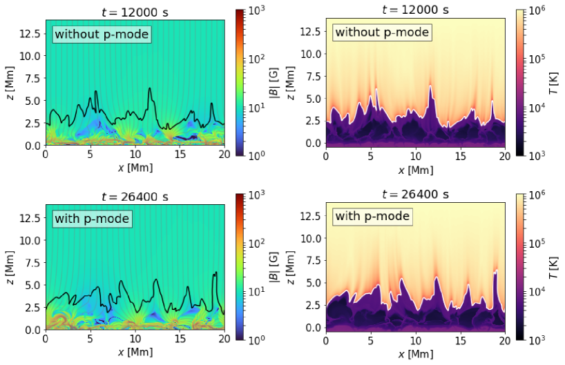
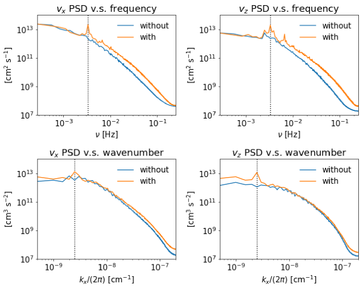
Figure 1 illustrates the velocity power spectra, denoted as and , as a function of frequency and wavenumber at . Here, , and these quantities are defined as follows:
| (11) | ||||
| (12) |
where the indices for the time () and horizontal () directions are denoted as and , respectively, with lengths and . We sampled frequencies () and horizontal wavenumbers () in increments of and , where represents the grid size in the direction (which is ), and is equal to . The power spectra exhibit sensitivity to the bottom boundary condition (i.e., with or without p-mode stages). The power spectra for the with p-mode stage exhibit distinct peaks at locations that correspond to the typical values of the p-modes, and .
2.2 Spicule Oscillation Analysis Method
Figure 2 displays the snapshots of the magnetic field and temperature distribution in both the without and with p-mode stages. After the relaxation of the convection, expanding magnetic flux tubes are formed of which footpoints are concentrated into kilogauss magnetic fields. In addition, Figure 2 reveals several spicule-like structures consisting of plasmas with chromospheric temperatures (). We utilize a fully automatic method with three steps to detect spicules and measure the period and velocity amplitude of the transverse oscillations in them. The method consists of the following steps:
-
1.
Identifying the spicules within the simulated data.
-
2.
Tracking the transverse oscillations of the identified spicules at a specific height.
-
3.
Deriving periods and velocity amplitudes of the spicule oscillations.
In constructing our three-step method, we draw upon the NUWT222Northumbria University Wave Tracking code as a reference (Morton et al., 2013; Thurgood et al., 2014; Weberg et al., 2018).
Step 1: We utilize an automated approach to identify spicules, considering them as local minima of temperature below across both temporal () and horizontal () dimensions at a specific height. Note that only local minima with widths in the -direction less than are categorized as spicules. This criterion aligns with the maximum spicule width observed in the quiet Sun atmosphere (Pasachoff et al., 2009). The lifetime of each spicule is determined by identifying the start and end times of the local minimum. In the left panel of Figure 3, a temperature map is displayed, emphasizing the edges of the spicule by white lines.
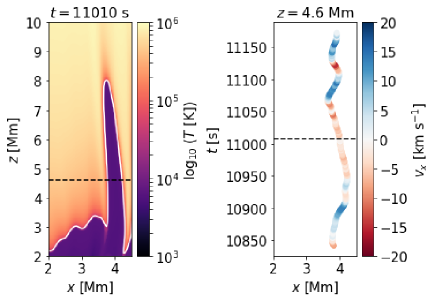
Step 2: At the given height and time, we calculate the mean horizontal () and perpendicular velocities (to the local magnetic field, ) between the right and left edges of the spicules. We then proceed to record the temporal evolution of them. In the right panel of Figure 3, we present an example of the recorded along the displacement, demonstrating an oscillatory pattern.
Step 3: To get the oscillation period, we utilize the fast Fourier transform (FFT) on the recorded temporal variation and generate the power spectra, denoted as , with respect to frequency defined as,
| (13) |
where , denotes the recorded velocity of the spicule during its lifetime, represents the sample size of for each spicule. We select the frequency to be that of the significant wave component, fulfilling the following condition:
| (14) |
Note that the frequency components which show at least of an oscillatory cycle are chosen. This approach leads to the selective detection of the high-frequency oscillations because it cannot identify oscillations with periods longer than the typical lifetime of spicules, which is on the order of a few minutes. The individual oscillation often exhibits multiple significant frequency components. We fit the time evolution of the horizontal velocity oscillations with a sinusoidal and linear function as
| (15) |
where the subscript expresses the individual wave component of the superposition, represents the number of oscillation modes chosen according to Equation (15), is the velocity amplitude, is the period (inverse of the selected frequency). We obtain , , , and through the fitting procedure.
3 Analysis and Results
3.1 Energy Transfer between Waves
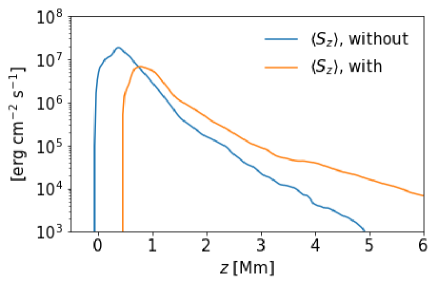
Figure 4 illustrates the distributions of the for the stages without and with p-modes, where
| (16) |
in the with p-mode stage is enhanced above compared to that in the without p-mode stage. In contrast, the increase in energy flux transported by longitudinal waves in the with p-mode stage initiates below as a consequence of the p-mode-like driver. (see Section 2.1). Therefore, the increase in signifies the transfer of energy from the longitudinal waves triggered by the driver to the transverse waves. It’s worth noting that in the with p-mode stage below z=0.5 Mm is negative because of the greater amplification of compared to . Due to the temporal and horizontal averaging applied to the energy fluxes, the amplification of likely involves multiple mechanisms, such as the mode conversion or mode absorption, which are local phenomena.
3.2 Statistical Properties of Spicule Oscillations
. without (mean standard error) with (mean standard error) height
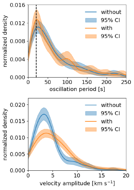
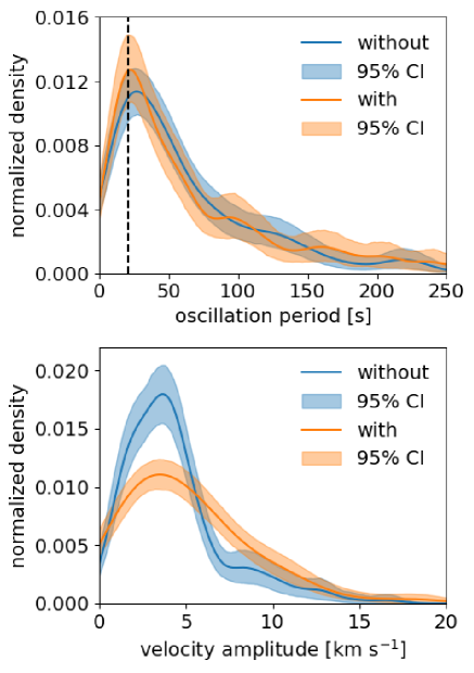
In this section, we investigate whether high-frequency spicule oscillations exhibit any signatures of energy transfer resulting from the longitudinal waves initiated by the p-mode-like driver, as shown in Section 3.1. We have applied our spicule oscillation analysis method at various heights, focusing on regions where the number of oscillations () is at least 100. This analysis encompasses heights up to , where in both the without and with stages, and the lowest height considered corresponds to the lower limit of spicule height observed in the quiet Sun (, Pasachoff et al., 2009). As an illustrative example, Figure 5 displays the density distributions of velocity amplitudes and oscillation periods at obtained from within the spicules. These distributions are estimated using kernel density estimation (KDE) with a Gaussian kernel. The bandwidth parameter is selected through cross-validation333Conducted using Scikit-learn (Pedregosa et al., 2011), following the same method as in Morton et al. (2021). The distributions of reveal a dominance of high-frequency (periods ) components in both stages with a peak around . Moreover, the distributions of demonstrate minimal difference between the two stages, while that of indicates an enhancement in the with p-mode stage compared to the without p-mode stage. These are common characteristics across all considered heights. The distributions of and obtained from and within the spicules exhibit a striking degree of similarity (see the distributions derived from as depicted in Figure 6 in the Appendix). This consistency arises primarily because a lot of spicules in our simulation are vertical due to our top boundary condition, which enforces a vertical magnetic field, i.e., , although some of them do exhibit clear inclinations.
At each of the heights investigated, we have computed the mean values of the oscillation period and velocity amplitude . Table 1 summarizes the oscillation parameters (, , and ) derived from perpendicular velocities within the detected spicules. Across different altitudes, there is no significant variation in mean parameters, and this remains within the range of standard errors. It is worth noting that the mean parameters derived from closely resemble those obtained from (refer to Table 3 in the Appendix). Furthermore, to assess the impact of the p-mode-like driver on the mean velocity amplitude, we have calculated the ratio of the mean velocity amplitude between the with and without p-mode stage, denoted as . The presence of the driver leads to an intensification of the mean velocity amplitudes by – (i.e., –) when using from and – (i.e., –) when using from . When we assess the increase in the power of velocity amplitude , we obtain – when using and – when using . This intensification exceeds the power of horizontal velocity at (, see Equation (10)). Hence, this result is unlikely to be solely attributed to the increase in horizontal velocity caused by the p-mode-like driver. Instead, it is more likely due to the energy transfer from the longitudinal wave energy generated by the driver to transverse wave energy, as explained in Section 3.1.
4 Discussion
The velocity amplitude of high-frequency spicule oscillations is enhanced by the presence of the p-mode-like driver. Therefore, despite accounting for the refraction of transverse (fast magnetic) waves, p-modes still have the potential to contribute to the production of high-frequency spicule oscillations, although the exact mechanism of the energy transfer cannot be definitively determined.
The distributions of oscillation periods for both stages exhibit a peak around . This value is consistent with the mean crossing time of acoustic waves across the equipartition layer, denoted as , which is expressed as follows (Shoda & Yokoyama, 2018):
| (17) |
in the without and with p-mode stage, as indicated by the dashed lines in the top panels of Figure 5. This result can be explained as follows: pulse-like amplifications in the velocity amplitude, lasting for approximately , are generated through the mode conversion at the equipartition layer (Schunker & Cally, 2006; Cally, 2007), as shown in Shoda & Yokoyama (2018). This finding is a consistent quantitative feature across all the heights we examined. However, it is important to note that this factor does not conclusively rule out the presence of other energy transfer systems, such as the mode absorption (Bogdan et al., 1996; Hindman & Jain, 2008; Riedl et al., 2019; Skirvin et al., 2023b).
Many observations employ the velocity amplitude of spicule oscillations to estimate the carried energy flux (Van Doorsselaere et al., 2014; Jess et al., 2023), using the following formula:
| (18) |
is obtained from the mean velocity amplitude of spicule transverse oscillations observed, while and are derived from various models (e.g., a bright network chromospheric model by Vernazza et al., 1981). Therefore, the squared value of the velocity amplitude serves as a primary indicator of the energy flux propagating within spicules. When we assume that all the obtained values of and represent the velocity amplitudes of propagating waves, the energy flux carried by them through spicules is amplified by – (i.e., –).
To analyze the nature of the detected oscillations, i.e., whether they are propagating or standing waves, we calculate their phase velocity as follows:
| (19) |
where represents the phase lag of the individual waves at two different heights ( and ), as obtained from Equation (15), and represents the height difference, i.e., . and are derived from within the spicules. To detect features of the same wave at different heights, we derive the properties of individual waves at a specific height and search for similar ones at an adjacent height, following the criteria of Bate et al. (2022). The considered properties (and criteria) include: (i) the -position of the spicule averaged over its lifetime (with a difference not exceeding , i.e., grids), (ii) the lifetime of the spicule (ensuring the duration of its existence between the considered heights overlaps), (iii) the duration of the oscillation (with a difference not exceeding ), and (iv) the oscillation period (with a difference not exceeding ). Based on these criteria, we have identified 13 upwardly propagating, 7 downwardly propagating, and 6 standing waves in the without p-mode stage. In the with p-mode stage, we have identified 6 upwardly propagating, 2 downwardly propagating, and 10 standing waves. Waves with a phase speed are classified as standing waves, following the same criteria applied by Okamoto & De Pontieu (2011). It should be noted that the number of the identified waves is much smaller than the total number of the detected oscillations . This is because the transverse waves in our two-dimensional simulation are fast mode waves, which propagate not only along but also across the magnetic field lines inside the spicules. Considering the obtained values of and in our simulation (averaged between those at and ) presented in Table 2, the energy flux propagating through spicules is intensified by around () for the upward waves and for the downward waves (). On the other hand, there is no clear increase for standing waves (i.e., ). Thus, propagating waves within spicules are significantly enhanced by the p-mode-like driver, while standing waves are not affected. However, care must be taken in the classification of the standing waves. Upwardly and downwardly propagating waves are superposed in the temporal evolutions of the spicule oscillations obtained by our method, potentially leading to misidentification of standing waves. The more sophisticated classification, achieved by filtering upwardly and downwardly propagating waves using spatiotemporal Fourier analysis (Tomczyk & McIntosh, 2009), may change the result.
| upward | downward | standing | |
|---|---|---|---|
| driver | |||
| without | |||
| with |
The oscillation periods obtained from horizontal velocities in simulated spicules (Figure 5) fall within the observed range of high-frequency spicule oscillations, as indicated by previous studies (Okamoto & De Pontieu, 2011; Bate et al., 2022). The velocity amplitudes of the simulated spicule oscillations (Table 1) are smaller than many observed values (median , Okamoto & De Pontieu, 2011; Pereira et al., 2012; Bate et al., 2022), while a few studies show good correspondence (Jafarzadeh et al., 2017; Yoshida et al., 2019). This discrepancy is likely to come from the top boundary condition in our simulation. In our simulation, the top boundary condition is implemented such that the magnetic field becomes vertical, i.e., , which consequently suppresses the transverse velocities of spicules.
The top boundary condition () also results in the reflection of transverse waves. To compare the energy flux carried by the reflected wave at the top boundary and the incident wave at the transition region, we have estimated them by using Equation (18). We verify that at the upper boundary is of that at the transition region in the absence of the p-mode-like driver, and in the presence of the driver. Hence, we can disregard the influence of the top boundary on the transverse spicule oscillations (i.e., below the transition region). However, the wave modulation in the corona arising from this reflection is not to be disregarded. Consequently, our numerical model does not have the capacity to investigate the generation of the peak observed in the coronal power spectra, as demonstrated in CoMP (Tomczyk et al., 2007; Tomczyk & McIntosh, 2009; Morton et al., 2015, 2019).
It is important to note that our two-dimensional simulation does not account for the three-dimensional effects such as the other mode conversion, responsible for generating Alfvén waves from fast waves (Cally & Goossens, 2008; Cally & Hansen, 2011; Hansen & Cally, 2012; Khomenko & Cally, 2012). In addition, spicules display three-dimensional motions, encompassing not only bulk transverse (kink-mode-like) oscillations but also rotational and cross-sectional oscillations (Sharma et al., 2017, 2018). These additional factors may indeed have an impact on the properties of high-frequency spicule oscillations produced by the p-modes. Further investigations using three-dimensional simulations are necessary to explore these effects in detail.
5 Conclusion
Our study focuses on examining the potential role of solar p-modes in generating high-frequency transverse spicule oscillations. To investigate this, we utilize a two-dimensional magneto-convection simulation that encompasses the upper convection zone to the corona. We introduce a driver in the middle of our simulation duration to generate longitudinal waves with periods and wavelengths resembling the typical values of p-modes.
We then proceed to analyze and compare the spicule oscillation characteristics between the stages without and with the p-mode-like driver. We find that the mean velocity amplitude increases by – by the driver, leading to the estimated enhancement of the energy flux in the spicules by –. This result implies that both p-modes and granulations play a substantial role in generating high-frequency spicule oscillations. Further investigations utilizing three-dimensional simulations are necessary to explore the contribution of p-modes to producing three-dimensional spicule transverse oscillations.
We would like to convey our sincere appreciation to the anonymous referee for providing valuable feedback. Numerical computations were carried out on the Cray XC50 at the Center for Computational Astrophysics (CfCA), National Astronomical Observatory of Japan. M.S. is supported by JSPS KAKENHI Grant Number JP22K14077. R.J.M. is supported by a UKRI Future Leader Fellowship (RiPSAW MR/T019891/1). H. K. is also grateful for travel support provided by the UKRI Future Leader Fellowship (RiPSAW MR/T019891/1). T.Y. is supported by the JSPS KAKENHI Grant Number JP21H01124, JP20KK0072, and JP21H04492. This work was supported by NAOJ Research Coordination Committee, NINS, Grant Number NAOJ-RCC-2301-0301.
Appendix A Additional Figures and Tables
Figure 6 shows the density distributions of velocity amplitudes and oscillation period of spicules similar to those shown in Figure 5, but obtained from horizontal velocities within the detected spicules. Table 3 presents the spicule oscillation parameters (, and ) derived from horizontal velocities.
| without (mean standard error) | with (mean standard error) | |||||
| height | ||||||
References
- Alfvén (1942) Alfvén, H. 1942, Nature, 150, 405, doi: 10.1038/150405d0
- Bate et al. (2022) Bate, W., Jess, D. B., Nakariakov, V. M., et al. 2022, ApJ, 930, 129, doi: 10.3847/1538-4357/ac5c53
- Beckers (1968) Beckers, J. M. 1968, Sol. Phys., 3, 367, doi: 10.1007/BF00171614
- Beckers (1972) —. 1972, ARA&A, 10, 73, doi: 10.1146/annurev.aa.10.090172.000445
- Bogdan et al. (1996) Bogdan, T. J., Hindman, B. W., Cally, P. S., & Charbonneau, P. 1996, ApJ, 465, 406, doi: 10.1086/177429
- Cally (2007) Cally, P. S. 2007, Astronomische Nachrichten, 328, 286, doi: 10.1002/asna.200610731
- Cally & Goossens (2008) Cally, P. S., & Goossens, M. 2008, Sol. Phys., 251, 251, doi: 10.1007/s11207-007-9086-3
- Cally & Hansen (2011) Cally, P. S., & Hansen, S. C. 2011, ApJ, 738, 119, doi: 10.1088/0004-637X/738/2/119
- Choudhuri et al. (1993) Choudhuri, A. R., Auffret, H., & Priest, E. R. 1993, Sol. Phys., 143, 49, doi: 10.1007/BF00619096
- Christensen-Dalsgaard (2002) Christensen-Dalsgaard, J. 2002, Reviews of Modern Physics, 74, 1073, doi: 10.1103/RevModPhys.74.1073
- Christensen-Dalsgaard et al. (1996) Christensen-Dalsgaard, J., Dappen, W., Ajukov, S. V., et al. 1996, Science, 272, 1286, doi: 10.1126/science.272.5266.1286
- Cranmer & van Ballegooijen (2010) Cranmer, S. R., & van Ballegooijen, A. A. 2010, ApJ, 720, 824, doi: 10.1088/0004-637X/720/1/824
- Cranmer & Winebarger (2019) Cranmer, S. R., & Winebarger, A. R. 2019, ARA&A, 57, 157, doi: 10.1146/annurev-astro-091918-104416
- De Moortel & Browning (2015) De Moortel, I., & Browning, P. 2015, Philosophical Transactions of the Royal Society of London Series A, 373, 20140269, doi: 10.1098/rsta.2014.0269
- De Pontieu et al. (2022) De Pontieu, B., Testa, P., Martínez-Sykora, J., et al. 2022, ApJ, 926, 52, doi: 10.3847/1538-4357/ac4222
- Dere et al. (1997) Dere, K. P., Landi, E., Mason, H. E., Monsignori Fossi, B. C., & Young, P. R. 1997, A&AS, 125, 149, doi: 10.1051/aas:1997368
- Deubner (1975) Deubner, F. L. 1975, A&A, 44, 371
- Edlén (1943) Edlén, B. 1943, ZAp, 22, 30
- Finley et al. (2022) Finley, A. J., Brun, A. S., Carlsson, M., et al. 2022, A&A, 665, A118, doi: 10.1051/0004-6361/202243947
- Fujimura & Tsuneta (2009) Fujimura, D., & Tsuneta, S. 2009, ApJ, 702, 1443, doi: 10.1088/0004-637X/702/2/1443
- Gabriel (1976) Gabriel, A. H. 1976, Philosophical Transactions of the Royal Society of London Series A, 281, 339, doi: 10.1098/rsta.1976.0031
- Gao et al. (2023) Gao, Y., Guo, M., Van Doorsselaere, T., Tian, H., & Skirvin, S. J. 2023, ApJ, 955, 73, doi: 10.3847/1538-4357/acf454
- Goodman & Judge (2012) Goodman, M. L., & Judge, P. G. 2012, ApJ, 751, 75, doi: 10.1088/0004-637X/751/1/75
- Grotrian (1939) Grotrian, W. 1939, Naturwissenschaften, 27, 214, doi: 10.1007/BF01488890
- Hansen & Cally (2012) Hansen, S. C., & Cally, P. S. 2012, ApJ, 751, 31, doi: 10.1088/0004-637X/751/1/31
- Hindman & Jain (2008) Hindman, B. W., & Jain, R. 2008, ApJ, 677, 769, doi: 10.1086/528956
- Iglesias & Rogers (1996) Iglesias, C. A., & Rogers, F. J. 1996, ApJ, 464, 943, doi: 10.1086/177381
- Iijima (2016) Iijima, H. 2016, PhD thesis, University of Tokyo, Department of Earth and Planetary Environmental Science
- Iijima & Yokoyama (2015) Iijima, H., & Yokoyama, T. 2015, ApJ, 812, L30, doi: 10.1088/2041-8205/812/2/L30
- Iijima & Yokoyama (2017) —. 2017, ApJ, 848, 38, doi: 10.3847/1538-4357/aa8ad1
- Jafarzadeh et al. (2017) Jafarzadeh, S., Solanki, S. K., Gafeira, R., et al. 2017, ApJS, 229, 9, doi: 10.3847/1538-4365/229/1/9
- Jess et al. (2023) Jess, D. B., Jafarzadeh, S., Keys, P. H., et al. 2023, Living Reviews in Solar Physics, 20, 1, doi: 10.1007/s41116-022-00035-6
- Jess et al. (2012) Jess, D. B., Pascoe, D. J., Christian, D. J., et al. 2012, ApJ, 744, L5, doi: 10.1088/2041-8205/744/1/L5
- Khomenko & Cally (2012) Khomenko, E., & Cally, P. S. 2012, ApJ, 746, 68, doi: 10.1088/0004-637X/746/1/68
- Klimchuk (2006) Klimchuk, J. A. 2006, Sol. Phys., 234, 41, doi: 10.1007/s11207-006-0055-z
- Klimchuk (2015) —. 2015, Philosophical Transactions of the Royal Society of London Series A, 373, 20140256, doi: 10.1098/rsta.2014.0256
- Kuniyoshi et al. (2023) Kuniyoshi, H., Shoda, M., Iijima, H., & Yokoyama, T. 2023, ApJ, 949, 8, doi: 10.3847/1538-4357/accbb8
- Landi et al. (2012) Landi, E., Del Zanna, G., Young, P. R., Dere, K. P., & Mason, H. E. 2012, ApJ, 744, 99, doi: 10.1088/0004-637X/744/2/99
- Leighton et al. (1962) Leighton, R. B., Noyes, R. W., & Simon, G. W. 1962, ApJ, 135, 474, doi: 10.1086/147285
- Lim et al. (2023) Lim, D., Van Doorsselaere, T., Berghmans, D., et al. 2023, ApJ, 952, L15, doi: 10.3847/2041-8213/ace423
- Mandal et al. (2022) Mandal, S., Chitta, L. P., Antolin, P., et al. 2022, A&A, 666, L2, doi: 10.1051/0004-6361/202244403
- Matsumoto (2016) Matsumoto, T. 2016, MNRAS, 463, 502, doi: 10.1093/mnras/stw2032
- McClure et al. (2019) McClure, R. L., Rast, M. P., & Martínez Pillet, V. 2019, Sol. Phys., 294, 18, doi: 10.1007/s11207-019-1395-9
- McIntosh et al. (2011) McIntosh, S. W., de Pontieu, B., Carlsson, M., et al. 2011, Nature, 475, 477, doi: 10.1038/nature10235
- Morton et al. (2023) Morton, R. J., Sharma, R., Tajfirouze, E., & Miriyala, H. 2023, Reviews of Modern Plasma Physics, 7, 17, doi: 10.1007/s41614-023-00118-3
- Morton et al. (2021) Morton, R. J., Tiwari, A. K., Van Doorsselaere, T., & McLaughlin, J. A. 2021, ApJ, 923, 225, doi: 10.3847/1538-4357/ac324d
- Morton et al. (2015) Morton, R. J., Tomczyk, S., & Pinto, R. 2015, Nature Communications, 6, 7813, doi: 10.1038/ncomms8813
- Morton et al. (2013) Morton, R. J., Verth, G., Fedun, V., Shelyag, S., & Erdélyi, R. 2013, ApJ, 768, 17, doi: 10.1088/0004-637X/768/1/17
- Morton et al. (2019) Morton, R. J., Weberg, M. J., & McLaughlin, J. A. 2019, Nature Astronomy, 3, 223, doi: 10.1038/s41550-018-0668-9
- Müller et al. (2020) Müller, D., St. Cyr, O. C., Zouganelis, I., et al. 2020, A&A, 642, A1, doi: 10.1051/0004-6361/202038467
- Musielak & Ulmschneider (2002) Musielak, Z. E., & Ulmschneider, P. 2002, A&A, 386, 606, doi: 10.1051/0004-6361:20011834
- Nisticò et al. (2013) Nisticò, G., Nakariakov, V. M., & Verwichte, E. 2013, A&A, 552, A57, doi: 10.1051/0004-6361/201220676
- Oba et al. (2017) Oba, T., Iida, Y., & Shimizu, T. 2017, ApJ, 836, 40, doi: 10.3847/1538-4357/836/1/40
- Okamoto & De Pontieu (2011) Okamoto, T. J., & De Pontieu, B. 2011, ApJ, 736, L24, doi: 10.1088/2041-8205/736/2/L24
- Pasachoff et al. (2009) Pasachoff, J. M., Jacobson, W. A., & Sterling, A. C. 2009, Sol. Phys., 260, 59, doi: 10.1007/s11207-009-9430-x
- Pedregosa et al. (2011) Pedregosa, F., Varoquaux, G., Gramfort, A., et al. 2011, Journal of Machine Learning Research, 12, 2825, doi: 10.48550/arXiv.1201.0490
- Pereira et al. (2012) Pereira, T. M. D., De Pontieu, B., & Carlsson, M. 2012, ApJ, 759, 18, doi: 10.1088/0004-637X/759/1/18
- Petrova et al. (2023) Petrova, E., Magyar, N., Van Doorsselaere, T., & Berghmans, D. 2023, ApJ, 946, 36, doi: 10.3847/1538-4357/acb26a
- Reale (2014) Reale, F. 2014, Living Reviews in Solar Physics, 11, 4, doi: 10.12942/lrsp-2014-4
- Riedl et al. (2019) Riedl, J. M., Van Doorsselaere, T., & Santamaria, I. C. 2019, A&A, 625, A144, doi: 10.1051/0004-6361/201935393
- Rochus et al. (2020) Rochus, P., Auchère, F., Berghmans, D., et al. 2020, A&A, 642, A8, doi: 10.1051/0004-6361/201936663
- Schrijver et al. (1997) Schrijver, C. J., Hagenaar, H. J., & Title, A. M. 1997, ApJ, 475, 328, doi: 10.1086/303528
- Schunker & Cally (2006) Schunker, H., & Cally, P. S. 2006, MNRAS, 372, 551, doi: 10.1111/j.1365-2966.2006.10855.x
- Sharma et al. (2017) Sharma, R., Verth, G., & Erdélyi, R. 2017, ApJ, 840, 96, doi: 10.3847/1538-4357/aa6d57
- Sharma et al. (2018) —. 2018, ApJ, 853, 61, doi: 10.3847/1538-4357/aaa07f
- Shimizu et al. (2022) Shimizu, K., Shoda, M., & Suzuki, T. K. 2022, ApJ, 931, 37, doi: 10.3847/1538-4357/ac66d7
- Shoda & Yokoyama (2018) Shoda, M., & Yokoyama, T. 2018, ApJ, 854, 9, doi: 10.3847/1538-4357/aaa54f
- Shrivastav et al. (2023) Shrivastav, A. K., Pant, V., Berghmans, D., et al. 2023, arXiv e-prints, arXiv:2304.13554, doi: 10.48550/arXiv.2304.13554
- Skirvin et al. (2023a) Skirvin, S., Verth, G., González-Avilés, J. J., et al. 2023a, Advances in Space Research, 71, 1866, doi: 10.1016/j.asr.2022.05.033
- Skirvin et al. (2023b) Skirvin, S. J., Gao, Y., & Van Doorsselaere, T. 2023b, ApJ, 949, 38, doi: 10.3847/1538-4357/acca7d
- Spitzer & Härm (1953) Spitzer, L., & Härm, R. 1953, Physical Review, 89, 977, doi: 10.1103/PhysRev.89.977
- Spruit (1981) Spruit, H. C. 1981, A&A, 98, 155
- Srivastava et al. (2017) Srivastava, A. K., Shetye, J., Murawski, K., et al. 2017, Scientific Reports, 7, 43147, doi: 10.1038/srep43147
- Stein & Nordlund (1998) Stein, R. F., & Nordlund, Å. 1998, ApJ, 499, 914, doi: 10.1086/305678
- Steiner et al. (1998) Steiner, O., Grossmann-Doerth, U., Knölker, M., & Schüssler, M. 1998, ApJ, 495, 468, doi: 10.1086/305255
- Sterling (2000) Sterling, A. C. 2000, Sol. Phys., 196, 79, doi: 10.1023/A:1005213923962
- Thurgood et al. (2014) Thurgood, J. O., Morton, R. J., & McLaughlin, J. A. 2014, ApJ, 790, L2, doi: 10.1088/2041-8205/790/1/L2
- Tian et al. (2012) Tian, H., McIntosh, S. W., Wang, T., et al. 2012, ApJ, 759, 144, doi: 10.1088/0004-637X/759/2/144
- Tomczyk & McIntosh (2009) Tomczyk, S., & McIntosh, S. W. 2009, ApJ, 697, 1384, doi: 10.1088/0004-637X/697/2/1384
- Tomczyk et al. (2007) Tomczyk, S., McIntosh, S. W., Keil, S. L., et al. 2007, Science, 317, 1192, doi: 10.1126/science.1143304
- Tomczyk et al. (2008) Tomczyk, S., Card, G. L., Darnell, T., et al. 2008, Sol. Phys., 247, 411, doi: 10.1007/s11207-007-9103-6
- Tsiropoula et al. (2012) Tsiropoula, G., Tziotziou, K., Kontogiannis, I., et al. 2012, Space Sci. Rev., 169, 181, doi: 10.1007/s11214-012-9920-2
- Ulrich (1970) Ulrich, R. K. 1970, ApJ, 162, 993, doi: 10.1086/150731
- Van Doorsselaere et al. (2014) Van Doorsselaere, T., Gijsen, S. E., Andries, J., & Verth, G. 2014, ApJ, 795, 18, doi: 10.1088/0004-637X/795/1/18
- Van Doorsselaere et al. (2020) Van Doorsselaere, T., Srivastava, A. K., Antolin, P., et al. 2020, Space Sci. Rev., 216, 140, doi: 10.1007/s11214-020-00770-y
- Vernazza et al. (1981) Vernazza, J. E., Avrett, E. H., & Loeser, R. 1981, ApJS, 45, 635, doi: 10.1086/190731
- Wang et al. (2012) Wang, T., Ofman, L., Davila, J. M., & Su, Y. 2012, ApJ, 751, L27, doi: 10.1088/2041-8205/751/2/L27
- Wang et al. (2021) Wang, Y., Yokoyama, T., & Iijima, H. 2021, ApJ, 916, L10, doi: 10.3847/2041-8213/ac10c7
- Wang (2020) Wang, Y. M. 2020, ApJ, 904, 199, doi: 10.3847/1538-4357/abbda6
- Wang (2022) —. 2022, Sol. Phys., 297, 129, doi: 10.1007/s11207-022-02060-y
- Weberg et al. (2018) Weberg, M. J., Morton, R. J., & McLaughlin, J. A. 2018, ApJ, 852, 57, doi: 10.3847/1538-4357/aa9e4a
- Yoshida et al. (2019) Yoshida, M., Suematsu, Y., Ishikawa, R., et al. 2019, ApJ, 887, 2, doi: 10.3847/1538-4357/ab4ce7
- Zhong et al. (2022) Zhong, S., Nakariakov, V. M., Kolotkov, D. Y., Verbeeck, C., & Berghmans, D. 2022, MNRAS, 516, 5989, doi: 10.1093/mnras/stac2545