Calibrated Multivariate Regression with Localized PIT Mappings
Abstract
Calibration ensures that predicted uncertainties align with observed uncertainties. While there is an extensive literature on recalibration methods for univariate probabilistic forecasts, work on calibration for multivariate forecasts is much more limited. This paper introduces a novel post-hoc recalibration approach that addresses multivariate calibration for potentially misspecified models. Our method involves constructing local mappings between vectors of marginal probability integral transform values and the space of observations, providing a flexible and model free solution applicable to continuous, discrete, and mixed responses. We present two versions of our approach: one uses K-nearest neighbors, and the other uses normalizing flows. Each method has its own strengths in different situations. We demonstrate the effectiveness of our approach on two real data applications: recalibrating a deep neural network’s currency exchange rate forecast and improving a regression model for childhood malnutrition in India for which the multivariate response has both discrete and continuous components.
Keywords: nearest neighbours, normalizing flows, probabilistic forecasting, regression calibration, uncertainty quantification
Acknowledgments: David Nott’s research was supported by the Ministry of Education, Singapore, under the Academic Research Fund Tier 2 (MOE-T2EP20123-0009), and he is affiliated with the Institute of Operations Research and Analytics at the National University of Singapore. Nadja Klein was supported by the Deutsche Forschungsgemeinschaft (DFG, German Research Foundation) through the Emmy Noether grant KL 3037/1-1.
1 Department of Statistics and Data Science, National University of Singapore, Singapore
2 Department of Statistics, University of Brasília, Brazil
3 School of Mathematics and Statistics, University of New South Wales, Australia
4 Scientific Computing Center, Karlsruhe Institute of Technology, Germany
∗ Correspondence should be directed to [email protected]
1 Introduction
Historically notions of calibration have their roots in probabilistic forecasting with applications in many fields. There are different types of calibration (e.g., Gneiting et al.; 2007), but heuristically a model is considered to be calibrated if its predicted uncertainty matches the observed uncertainty in the data in some sense. For example, a forecast might be considered useful for decision making if an event with a certain forecast probability occurs with the corresponding relative frequency. Calibration of probabilistic models is considered desirable in many scenarios, and has been studied for many types of models and applications, such as neural networks (Dheur and Ben Taieb; 2023; Lakshminarayanan et al.; 2017), regression (Klein et al.; 2021), simulator based inference (Rodrigues et al.; 2018), and clustering (Guo et al.; 2017). In many situations probabilistic forecasts can be multivariate, involving a vector of random variables . However, ensuring multivariate calibration is a challenging task. In this paper, we introduce a novel approach to recalibrating uncertainties obtained from multivariate probabilistic forecasts, based on models which are possibly misspecified. Our approach can be applied post hoc to arbitrary and already fully fitted models ensuring approximate multivariate calibration while simultaneously keeping other properties such as the interpretability of the base model intact. While we focus on recalibrating an existing base model, it is possible to use a very flexible model at the outset, and there is an extensive literature on flexible regression beyond the mean (Kneib; 2013; Henzi et al.; 2021).
To explain our contribution, it is necessary to discuss different types of calibration. For univariate responses, a common choice is probability calibration (Gneiting et al.; 2007), which can be assessed by checking uniformity of the probability integral transform (PIT) values (Dawid; 1984). A PIT value is the evaluation of the cumulative distribution function (CDF) of the model at an observed data point. Uniformity of the PIT values implies that prediction intervals derived from the probabilistic model have the correct coverage in a frequentist sense. When extending probability calibration from the univariate to the multivariate setting, it is not enough to check uniformity of PIT values for each marginal separately.
Smith (1985) considers joint uniformity of the univariate PIT values under a Rosenblatt transformation (Rosenblatt; 1952) summarizing the joint distribution. Diebold et al. (1998) suggest to check this graphically using histograms and correlograms, and formal tests have been developed in the context of economic forecasting (Corradi and Swanson; 2006; Ko and Park; 2013; Dovern and Manner; 2020). However, this approach is limited, as a Rosenblatt transformation is not readily available for many complex models.
In the context of ensemble forecasts, Gneiting et al. (2008) introduce multivariate rank histograms as a simple graphical check for multivariate calibration. Multivariate rank histograms are extended to copula PIT (CopPIT) values by Ziegel and Gneiting (2014). If all univariate marginals of the prediction model are probability calibrated, the CopPIT values depend only on the copula of the forecast. A formal description of this is given in Section 2. An alternative to PIT and CopPIT values are proper scoring rules (Gneiting and Raftery; 2007), which jointly quantify calibration and sharpness of a probabilistic prediction model. Formal tests for multivariate calibration based on scoring rules complementing PIT-based calibration can be derived (Knüppel et al.; 2023).
Even when useful in practice, many models suffer from miscalibration induced by model misspecification. For example, computer based simulators idealise and simplify complex real world phenomena and thus suffer from model misspecification (Ward et al.; 2022); in regression, highly structured, but therefore misspecified models can be preferable when the focus is on interpretation and not on prediction; modern deep neural networks suffer from several sources of uncertainty that can be challenging to track through their complex structures (Gawlikowski et al.; 2023). These observations motivate recalibration techniques, which allow to adjust a fitted model post hoc.
When it comes to recalibration of already estimated models, a rich literature exists in the univariate context. The approaches are often tailored to a specific subclass of statistical models. In the context of parameter estimation, Menéndez et al. (2014) consider recalibration of confidence intervals using bootstrap style samples generated from a predictive distribution under the estimated model. In classification, Platt-scaling (Platt; 1999), which extends a trained classifier with a logistic regression model to return class probabilities, is a popular approach. Platt-scaling has been extended in various directions within the machine learning literature (e.g., Guo et al.; 2017; Kull et al.; 2017). For univariate regression, Kuleshov et al. (2018) suggest learning a transformation of the PIT values to achieve probability calibration. They use isotonic regression and their approach is extended by Dheur and Ben Taieb (2023), who use a kernel density estimator (KDE) of the PIT distribution instead. Our approach can be considered as a multivariate extension to this idea and we review it in more detail in Section 2.1. Our approach is also closely linked to the local recalibration technique for artificial neural networks proposed by Torres et al. (2024). They use non-parametric PIT transformations on a local neighbourhood learned with K-nearest neighbours (KNN), which can be applied to any layer of a deep neural architecture.
Despite the clear need, there is still a lack of general multivariate recalibration techniques that consider a vector of quantities of interest jointly in the literature. Heinrich et al. (2021) discuss post-processing methods for multivariate spatio-temporal forecasting models. However, calibration is only one of their many objectives and the approach does not easily generalize to other model classes. Recently, Wehenkel et al. (2024) considered recalibration for simulation-based inference under model misspecification. Their approach involves learning an optimal transport map between real world observations and the output of the misspecified simulator.
The main contributions of this paper are as follows. (i) We introduce a novel method to achieve multivariate calibration post hoc. The main idea is to construct local mappings between vectors of marginal PIT values and the observation space. Our method thus complements established methods for univariate calibration. (ii) Our approach is general. We are not restricted to continuous data, but can consider discrete and even mixed responses. Therefore the approach can be applied beyond regression to tasks such as clustering, classification, and generalized parameter inference. (iii) Our approach is model-free as we do not assume a particular structure of the underlying base model. Even though it is helpful if the CDFs of the univariate marginals are available in closed form, our method can be applied as long as samples from the base model can be readily generated. (iv) Our method is simple to use. We introduce two versions of our approach. First, a KNN-based approach similar to Torres et al. (2024), which is then extended to a normalizing flow based approach, where the PIT maps are explicitly learned. Both versions of our approach come with different advantages and we discuss which method is best suited to which scenario.
We apply our method to two real data examples. First, we recalibrate a one-day ahead forecast for currency exchange rates based on a deep neural network. Multivariate calibration, where all currencies are considered jointly, is desirable due to the complex dependence structure across currencies. Secondly, we consider a regression task concerning childhood malnutrition in India. The bivariate response vector is mixed, containing a continuous and a discrete response. Multivariate recalibration can be used to combine univariate regression models into one joint predictor. Specifying separate regression models for the predictors can be easier then constructing a joint model, especially when working with mixed data.
The rest of this paper is organized as follows. First, we give some background on different definitions of calibration and existing recalibration techniques in Section 2. Then, we present our novel recalibration method in Section 3. Section 4 illustrates the good performance of our approach for simulated data in a number of scenarios and Section 5 considers the aforementioned real data examples. Section 6 gives a concluding discussion.
2 Background on Calibration
Let denote the joint distribution of a response and feature vector . In practice, is unknown and the conditional distribution is estimated by some probabilistic model from a training set . Heuristically, the model is said to be calibrated if it correctly specifies the uncertainty in it’s own predictions. Since is not available in practice, calibration can only be assessed based on a validation set of observations from , which is potentially disjoint from . In this section, we will give some background on the notion of calibration by first reviewing univariate calibration in Section 2.1, which will be then extended to the multivariate setting in Section 2.2.
2.1 Univariate Calibration
In the univariate case, where , several notions of calibration exist within the literature (e.g., Gneiting and Resin; 2023). Here, we focus on marginal calibration and probability calibration, which are two choices commonly considered in practice.
is said to be marginally calibrated (Gneiting et al.; 2007) if
That is, the average predictive CDF matches with the empirical CDF of the observations asymptotically for all . Hence, Gneiting et al. (2007) suggest plotting the average predictive CDF versus the empirical CDF to graphically assess marginal calibration.
The random variable
| (1) |
where and is the left-handed limit of as approaches from below, is the randomized PIT value (Czado et al.; 2009). Note that depends both on and the model . If is continuous, is not randomized
is said to be probability calibrated if . For let be independent uniform random variables on and write
| (2) |
is an empirical evaluation of (1) across the validation set. Thus, probability calibration can be graphically checked by plotting a histogram of . Formal tests for uniformity of the PIT values based on the Wasserstein distance (Zhou et al.; 2021; Zhao et al.; 2020) and the Cramér-von Mises distance (Kuleshov et al.; 2018) are popular alternatives to graphical checks. Gneiting et al. (2007) show that probability calibration is under mild conditions equivalent to quantile calibration (Kuleshov et al.; 2018), which requires
where denotes the generalized inverse of . This perspective has the nice interpretation that prediction intervals derived from have the correct coverage.
Histograms of the PIT values can also be used for model criticism as they indicate the type of miscalibration at hand. For example, U-shaped histograms indicate overconfidence, while triangular shapes indicate a biased model (Gneiting et al.; 2007).
Several techniques to recalibrate a potentially miscalibrated model in a post-hoc step exist in the literature. Here, we describe a simple method for doing this due to Kuleshov et al. (2018). Write for the distribution function of the PIT values (1), where dependence on and is left implicit in the notation. It is easy to check that is a distribution function for every and probability calibrated with respect to . In practice, the distribution function is not known, and it must be estimated from . Kuleshov et al. (2018) suggest using a method based on isotonic regression. Dheur and Ben Taieb (2023) extend this idea and consider KDEs. Among other choices, they propose to use
which is the empirical CDF from the PIT values over the validation set . An alternative approach to recalibration for regression models is given by Song et al. (2019). Recently, Torres et al. (2024) proposed nonparametric local recalibration for neural networks. Their approach uses a fast KNN algorithm to localize the recalibration and can be used in any layer of the neural network scaling to potentially high-dimensional feature spaces .
2.2 Multivariate Calibration
Extending the different notions of calibration from the univariate to the multivariate case, , is not straightforward. One reason for this is that the multivariate integral transformation
is, in contrast to the univariate case, generally not uniformly distributed (e.g., Genest and Rivest; 2001), but follows the so-called Kendall distribution of . The Kendall distribution depends only on the copula of the multivariate probability measure, and thus summarizes the dependence structure of . Based on this observation, Ziegel and Gneiting (2014) introduce copula probability integral transform (CopPIT) values as analogous to the univariate PIT values described in (1). The CopPIT values are given as
| (3) |
where , , and denotes the Kendall distribution of . is said to be copula calibrated if the CopPIT values are uniformly distributed on the unit interval (Ziegel and Gneiting; 2014). In this way, copula calibration can be seen as a multivariate extension to probability calibration. In particular for , is the uniform distribution on , so that (3) is equal to . As in the univariate case, let
denote the empirical CopPIT values from the validation set, , where are independent uniform variates on . Again, copula calibration can be assessed by checking uniformity of . However, interpretation of the CopPIT histograms is more challenging than in the univariate case, as they not only summarize potential miscalibration of the dependence structure, but also of the marginal distributions. However, in the special case that all margins of are uniformly probability calibrated, the CopPIT values summarize miscalibration of the copula of only (Ziegel and Gneiting; 2014). Thus, in practice it is sensible to assess multivariate calibration by checking for univariate calibration of each marginal in terms of the marginal PIT values (1) and copula calibration in terms of the CopPIT values (3).
Ziegel and Gneiting (2014) also introduce Kendall calibration
| (4) |
as the multivariate analogue to marginal calibration. Kendall calibration can be assessed by a so called Kendall diagram, which is a scatter plot of the empirical left hand side versus the empirical right hand side of (4) for different values of .
Both copula calibration and Kendall calibration necessitate the derivation of the Kendall distributions . The Kendall distribution can be calculated in closed form only for a few special cases (e.g., Genest and Rivest; 2001). So, in practice, in (3) and (4) is replaced by an approximation given as the empirical CDF of the pseudo observations (Barbe et al.; 1996)
where if for all and is a large sample from .
3 Multivariate Calibration via PIT mapping
This section describes our approach to recalibrate arbitrary probabilistic prediction models . We consider a simple KNN approach, which can be thought of as a multivariate extension to the recalibration methods by Torres et al. (2024) and Rodrigues et al. (2018) first in Section 3.1, and then the novel normalizing flow based method in Section 3.2.
3.1 Nearest neighbour recalibration
Suppose that we have a mapping on the feature space, . The purpose of the function is to reduce the dimension of and we use to measure the similarity of the feature vectors and . Let
If is a sufficiently small neighbourhood around , approximates a sample from , where is the PIT value for the -th response of as given in (1). Let denote the joint distribution of given with marginal distributions , . Theoretical properties of were studied in Rodrigues et al. (2018). In particular, has probability calibrated marginals following the same arguments as for the univariate recalibration techniques described in Section 2.1. Note that the use of instead of the global unconditional distribution as considered in Kuleshov et al. (2018) and Dheur and Ben Taieb (2023) gives a stronger form of calibration, as the resulting model is locally, that is conditional on , probability calibrated. In addition to the marginal information, also matches the dependence structure of under . For a given and continuous marginals , is a non-random transformation of and, in particular, is an invertible transformation of . The Kendall distribution is invariant under such transformations and thus the CopPIT value could be calculated purely on , without access to . Also, has copula , which is the copula of and, from the arguments above, has probability calibrated marginals. Following Ziegel and Gneiting (2014) this implies copula calibration.
Thus, for a given , a sample of size from an approximately calibrated predictive distribution can be generated as
| (5) |
Here, with the empirical PIT value for the -th marginal distribution evaluated on the -th entry of the validation set. If is not available in closed form it can be easily approximated using a sample from making our approach model free.
3.2 Recalibration with normalizing flows
We can think of the nearest neighbour approach introduced in Section 3.1 as obtaining an approximate sample from for a target feature vector , and then transforming back to the original space of the responses to obtain approximate samples of . In the nearest neighbour approach, no explicit expression for is constructed, and the number of potential draws from is restricted by heavily depending on . However, some applications require calculating complex summary statistics from the potentially intricate distribution , which necessitates the ability to draw arbitrary large samples from the recalibrated model. Thus, we propose a similar method to the KNN approach using normalizing flows to draw approximate samples from .
The basic idea is as follows. Let be a reference density with respect to the Lebesgue measure on , which we take to be the standard normal density. We consider a bijective transformation , and transform to a random vector , where is a set of learnable parameters. The density of is thus approximated as
where is the inverse of , and is its Jacobian matrix. Based on this, the parameter is learned using observations , where denotes the vector of PIT values for the marginal distributions evaluated on the validation set. To avoid boundary effects, we consider normalized PIT values , where is the CDF of the standard Gaussian distribution, instead of the usual PIT values on . As for the KNN approach, can be replaced with a lower dimensional representation in the construction of . Having learned as , samples from can be generated by sampling and setting . These samples can be then used similar to (5) to generate samples from the approximately recalibrated predictive distribution . Pseudo code for the full approach is given in Appendix A.
There are many ways to construct suitable transformations in the literature on transport maps (e.g., Marzouk et al.; 2016) and normalizing flows (e.g., Rippel and Adams; 2013; Yao et al.; 2023) as well as standard software for conditional density estimation. Here, we consider the real-valued non-volume preserving (real-NVP) approach by Dinh et al. (2017), where is given as a stack of affine coupling layers. We found this to be a satisfactory choice in all examples considered, but alternative approaches might be better suited depending on the structure of the recalibration task at hand.
The normalizing flow can be interpreted as a conditional density estimate for . If , our approach can therefore be considered a localized version of the KDE based method by Dheur and Ben Taieb (2023).
4 Simulations
We illustrate the performance of both the KNN based approach labeled KNN, and the normalizing flow approach labeled NF on a number of simulated examples. First, we reanalyze the illustrative example from Ziegel and Gneiting (2014) to consider forecasts suffering different kinds of miscalibration. Both KNN and NF achieve probability calibration of the marginals, copula calibration and Kendall calibration across all scenarios. Secondly, we consider a regression task, where is degenerate and we investigate the local calibration properties of our approaches. For a given , both NF and KNN allow to generate samples from the recalibrated predictive distribution . KNN can generate only a small sample of size much smaller then , while NF is computational more complex, but allows to draw an arbitrarily large sample from the recalibrated model. In our simulations, samples from both methods are close to the true distribution even for a grossly misspecified base model. More details on the simulation studies can be found in Appendix B.
5 Applications
5.1 Currency exchange rates
Foreign currencies constitute a popular class of assets among investors. In so-called Forex trading, traders exchange currencies with the goal of making a profit. The ability to make reliable predictions for currency exchange rates is crucial for a successful trading strategy. To this end, we analyze five time series of daily exchange rates for five currencies relative to the US dollar: the Australian Dollar (AUD), the Chinese Yuan (CNY), the Euro (EUR), the Pound Sterling (GBP), and the Singapore Dollar (SGD). These data span five years from August 01, 2019, to August 01, 2024, and were sourced from Yahoo Finance. Given the high correlation among currency exchange rates, multivariate calibration is a desirable feature for any currency exchange forecasting model.
Baseline model
We consider a one-day ahead forecast based on a Long Short-Term Memory (LSTM) Neural Network with a distributional layer, so that the resulting forecast distribution is multivariate Gaussian with diagonal covariance structure. Even though the resulting probabilistic forecast cannot express correlation, dependencies between the currencies are exploited through the deep LSTM network modelling the -dimensional time-series jointly. LSTMs have been successfully implemented for time-series prediction (e.g., Hua et al.; 2019) and the resulting model recovers the general structure of the data well. Note however that our main focus is to illustrate the merits of multivariate calibration and not on the construction of the forecasting model.
Recalibration in online learning
Every day, as a new data point becomes available, the baseline LSTM model is updated accordingly. The recalibration model follows a similar iterative process. After an initial period (here 100 days), the process is as follows. The LSTM model generates a predictive distribution for the one-day-ahead forecast. This forecast is then recalibrated using the recalibration model. Once the actual data for the next day is obtained, the LSTM model is updated on the now extended dataset. Simultaneously, the new data point yields an updated vector of marginal PIT values, prompting an update to the recalibration model. In each step only one additional data point becomes available, and both the base and the recalibration model can be updated using a warm-start avoiding the need to retrain the models from scratch. This drastically reduces the computational resources needed for training. We do not use a separate validation set, but reuse the training data for recalibration of the forecast.
In time series forecasting, a natural assumption is that the more recent an observation was made, the more information it contains on future values. Hence, here we consider the KNN approach, where we use the most recent 100 PIT values for recalibration at each time step. This way, the recalibration is carried out on a rolling window of PIT values. The KNN approach is preferable to NF here as it allows us to gradually control the information available to the recalibration method.
Results
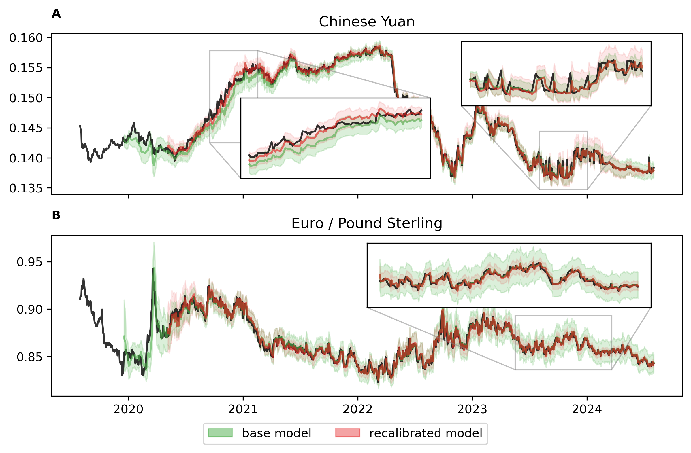
Histograms of the univariate PIT values (Appendix C) indicate that none of the margins of the base model are probability calibrated, and the kind of miscalibration differs drastically between currencies. For example, the marginal PIT values for CNY and SGD are skewed indicating a biased forecast, while the histograms for AUD and EUR are U shaped indicating underdispersion (Gneiting et al.; 2007). The recalibration through KNN drastically improves the overall calibration of the base model. Figure 1A shows the base, and the recalibrated forecast together with the realized values for CNY. The base model underestimates the exchange rate for CNY in 2020 and 2021. This bias is corrected by the recalibration. In the third and fourth quarter of 2023, the base model underestimates the uncertainty of the forecast, resulting in an accumulation of realised values outside of the credible band during this time period. Our KNN approach detects this local miscalibration and widens the credible band in this time period. Multivariate calibration is especially helpful when estimating functions over multiple margins, as done for example when assessing the risk of a portfolio. To illustrate this, we consider the time-series EUR/GBP, which gives the direct exchange rate for EUR relative to GBP. Both the base and the recalibrated forecast model describe an implicit forecast for EUR/GBP. EUR and GBP are strongly correlated with an estimated Kendall’s of . Since the base model does not account for this dependence structure, the estimated credible intervals are wider than necessary. Even though KNN does not recalibrate EUR/GBP directly, this is corrected by the multivariate recalibration as shown in Figure 1B.
5.2 Childhood malnutrition
Ending all forms of malnutrition is one of the sustainable development goals of the United Nations (United Nations; 2015). Here, we consider a sample from the Demographic and Health surveys (www.measuredhs.com) containing observations on several factors of undernutrition in India. Following previous analyses of the data (Klein et al.; 2020; Briseño Sanchez et al.; 2024) we consider two responses. The continuous indicator wasting reports weight for height as a z-score and the binary response fever indicates fever within the two weeks prior to the interview. Following Klein et al. (2020) we consider the covariables csex indicating the sex of the child, cage the age of the child in months, breastfeeding the duration of breastfeeding in months, mbmi the body mass index of the mother, and dist the district in India the child lives in.
Baseline model
We fit separate regression models for the two responses. wasting is modelled through a heteroscedastic Gaussian distribution, where both the mean and the variance parameter are linked to an additive predictor, and we use logistic regression for fever. Non-linear effects for the continuous covariates cage, breastfeeding, and mbmi are modelled with Bayesian P-splines (Eilers and Marx; 1996). We use a linear effect for csex, and a spatial effect with a Gaussian Markov random field prior for dist (Rue and Held; 2005). This results in two highly interpretable distributional regression models.
Multivariate calibration
Figure 2A shows a scatter plot of the normalized PIT values for the independent baseline regression models. While the PIT values for fever under the logistic regression model are close to the uniform distribution, the PIT values for wasting show clear deviations from uniformity especially in the upper tail. Since both fever and wasting are indicators of the child’s health, a complex dependence structure between the two response variables that is not sufficiently accounted for by the baseline model is expected. Multivariate calibration is used to combine the two univariate distributional regression models into a single multivariate regression model. Since we want to investigate how the recalibration affects the interpretable effects of the univariate regression models, we need to be able to generate large samples from , which is not possible with the basic KNN approach. We will thus consider the NF approach as described in Section 3. We condition the NF on the continuous covariables cage, and mbmi as they are predominant factors in the marginal regression models.
Results
The NF improves both the probabilistic calibration of the marginals and the copula calibration of the bivariate regression model as described by the PIT and CopPIT values respectively (Appendix C). The World Health Organization defines a child suffering from wasting if . Figure 2B shows the left tail for the predictive density of wasting conditional on the median values for all covariables for both the baseline and the recalibrated model. The baseline model overestimates the risk of the median child suffering wasting compared to the recalibrated model.
The joint regression model allows us to study the risk of a child having fever and simultaneously suffering from wasting . Figures 2C and D show the main effects of cage and dist on this risk respectively. The main effects are calculated by varying the covariable of interest, while keeping the other covariables fixed to their median values. The risk increases for children younger than a year and decreases for older children. The likelihood for fever is increasing for according to the baseline logistic regression model. Both the baseline and the recalibrated model find similar shapes for the main effect for cage, but in terms of magnitude the recalibrated model estimates a lower risk. Similarly, the estimated main effect for dist is lower for the recalibrated model than for the baseline model in all 438 districts (Appendix C). According to this analysis the risk of a child suffering simultaneously from wasting and fever is higher in the mid-eastern districts of India. This is consistent with the findings in Briseño Sanchez et al. (2024). Even though the recalibrated model is nonparametric, the interpretability of the baseline regression models can be maintained, making the multivariate recalibration approach a valuable tool for the development of complex multivariate distributional regression models.

6 Conclusion and Discussion
In this paper, we have introduced a novel approach for recalibrating multivariate models, addressing a critical gap in the calibration literature. Our method involves local mappings between marginal PIT values and the space of the observations and extends established univariate recalibration techniques to the multivariate case. We discuss two different versions of our approach. The KNN-based method provides simplicity and ease of implementation, but is limited as it only allows the generation of a small sample from the recalibrated model. While being computationally more challenging, the NF-based method overcomes this limitation. The merits of our approach are illustrated on a number of simulated and real data examples. We consider forecasting of a multivariate time series and regression for mixed data, further illustrating the versatility of our approach. However, theoretical properties of the PIT-based mappings are not well investigated. A better theoretical understanding could potentially lead to improved recalibration techniques. We use transformations of the PIT values from the marginal distributions. However, depending on the structure of the underlying predictor model, other univariate distributions that summarize the joint distribution could be considered. Future research could investigate the application of our recalibration technique to additional model types, including more intricate dependence structures and larger datasets. Additionally, our method focuses purely on calibration, and integrating it with other aspects of model evaluation and improvement, such as sharpness and robustness checks, could enhance its utility. Calibration is also an important tool for model criticism. The local nature of our approach could potentially allow to detect areas of model misspecification and thus our approach could be developed further into model specification and model selection pipelines.
References
- (1)
- Barbe et al. (1996) Barbe, P., Genest, C., Ghoudi, K. and Rémillard, B. (1996). On Kendall’s process, Journal of multivariate analysis 58(2): 197–229.
- Briseño Sanchez et al. (2024) Briseño Sanchez, G., Klein, N., Klinkhammer, H. and Mayr, A. (2024). Boosting distributional copula regression for bivariate binary, discrete and mixed responses, arXiv preprint arXiv:2403.02194 .
- Corradi and Swanson (2006) Corradi, V. and Swanson, N. R. (2006). Predictive density evaluation, Handbook of Economic Forecasting 1: 197–284.
- Czado et al. (2009) Czado, C., Gneiting, T. and Held, L. (2009). Predictive model assessment for count data, Biometrics 65(4): 1254–1261.
- Dawid (1984) Dawid, A. P. (1984). Statistical theory: The prequential approach (with discussion and rejoinder), Journal of the Royal Statistical Society, Series A 147: 278–292.
- Dheur and Ben Taieb (2023) Dheur, V. and Ben Taieb, S. (2023). A large-scale study of probabilistic calibration in neural network regression, in A. Krause, E. Brunskill, K. Cho, B. Engelhardt, S. Sabato and J. Scarlett (eds), Proceedings of the 40th International Conference on Machine Learning, Vol. 202 of Proceedings of Machine Learning Research, PMLR, pp. 7813–7836.
- Diebold et al. (1998) Diebold, F., Gunther, T. A. and Tay, A. S. (1998). Evaluating density forecasts with applications to financial risk management, International Economic Review 39(4): 863–83.
-
Dinh et al. (2017)
Dinh, L., Sohl-Dickstein, J. and Bengio, S. (2017).
Density estimation using real NVP, 5th International
Conference on Learning Representations, ICLR 2017, Toulon, France, April
24-26, 2017, Conference Track Proceedings, OpenReview.net.
https://openreview.net/forum?id=HkpbnH9lx - Dovern and Manner (2020) Dovern, J. and Manner, H. (2020). Order-invariant tests for proper calibration of multivariate density forecasts, Journal of Applied Econometrics 35(4): 440–456.
- Eilers and Marx (1996) Eilers, P. H. and Marx, B. D. (1996). Flexible smoothing with B-splines and penalties, Statistical Science 11(2): 89–121.
- Gawlikowski et al. (2023) Gawlikowski, J., Tassi, C. R. N., Ali, M., Lee, J., Humt, M., Feng, J., Kruspe, A., Triebel, R., Jung, P., Roscher, R. et al. (2023). A survey of uncertainty in deep neural networks, Artificial Intelligence Review 56(Suppl 1): 1513–1589.
- Genest and Rivest (2001) Genest, C. and Rivest, L.-P. (2001). On the multivariate probability integral transformation, Statistics & probability letters 53(4): 391–399.
- Gneiting et al. (2007) Gneiting, T., Balabdaoui, F. and Raftery, A. E. (2007). Probabilistic forecasts, calibration and sharpness, Journal of the Royal Statistical Society Series B: Statistical Methodology 69(2): 243–268.
- Gneiting and Raftery (2007) Gneiting, T. and Raftery, A. E. (2007). Strictly proper scoring rules, prediction, and estimation, Journal of the American statistical Association 102(477): 359–378.
- Gneiting and Resin (2023) Gneiting, T. and Resin, J. (2023). Regression diagnostics meets forecast evaluation: Conditional calibration, reliability diagrams, and coefficient of determination, Electronic Journal of Statistics 17(2): 3226–3286.
- Gneiting et al. (2008) Gneiting, T., Stanberry, L. I., Grimit, E. P., Held, L. and Johnson, N. A. (2008). Assessing probabilistic forecasts of multivariate quantities, with an application to ensemble predictions of surface winds, Test 17: 211–235.
- Guo et al. (2017) Guo, C., Pleiss, G., Sun, Y. and Weinberger, K. Q. (2017). On calibration of modern neural networks, in D. Precup and Y. W. Teh (eds), Proceedings of the 34th International Conference on Machine Learning, Vol. 70 of Proceedings of Machine Learning Research, PMLR, pp. 1321–1330.
- Heinrich et al. (2021) Heinrich, C., Hellton, K. H., Lenkoski, A. and Thorarinsdottir, T. L. (2021). Multivariate postprocessing methods for high-dimensional seasonal weather forecasts, Journal of the American Statistical Association 116(535): 1048–1059.
- Henzi et al. (2021) Henzi, A., Ziegel, J. F. and Gneiting, T. (2021). Isotonic Distributional Regression, Journal of the Royal Statistical Society Series B: Statistical Methodology 83(5): 963–993.
- Hua et al. (2019) Hua, Y., Zhao, Z., Li, R., Chen, X., Liu, Z. and Zhang, H. (2019). Deep learning with long short-term memory for time series prediction, IEEE Communications Magazine 57(6): 114–119.
- Klein et al. (2020) Klein, N., Kneib, T., Marra, G. and Radice, R. (2020). Bayesian mixed binary-continuous copula regression with an application to childhood undernutrition, Flexible Bayesian Regression Modelling, Elsevier, pp. 121–152.
- Klein et al. (2021) Klein, N., Nott, D. J. and Smith, M. S. (2021). Marginally calibrated deep distributional regression, Journal of Computational and Graphical Statistics 30(2): 467–483.
- Kneib (2013) Kneib, T. (2013). Beyond mean regression, Statistical Modelling 13(4): 275–303.
- Knüppel et al. (2023) Knüppel, M., Krüger, F. and Pohle, M.-O. (2023). Score-based calibration testing for multivariate forecast distributions, arXiv preprint arXiv:2211.16362 .
- Ko and Park (2013) Ko, S. I. and Park, S. Y. (2013). Multivariate density forecast evaluation: a modified approach, International Journal of Forecasting 29(3): 431–441.
- Kuleshov et al. (2018) Kuleshov, V., Fenner, N. and Ermon, S. (2018). Accurate uncertainties for deep learning using calibrated regression, in J. Dy and A. Krause (eds), Proceedings of the 35th International Conference on Machine Learning, Vol. 80 of Proceedings of Machine Learning Research, PMLR, pp. 2796–2804.
- Kull et al. (2017) Kull, M., Filho, T. S. and Flach, P. (2017). Beta calibration: a well-founded and easily implemented improvement on logistic calibration for binary classifiers, in A. Singh and J. Zhu (eds), Proceedings of the 20th International Conference on Artificial Intelligence and Statistics, Vol. 54 of Proceedings of Machine Learning Research, PMLR, pp. 623–631.
- Lakshminarayanan et al. (2017) Lakshminarayanan, B., Pritzel, A. and Blundell, C. (2017). Simple and scalable predictive uncertainty estimation using deep ensembles, in I. Guyon, U. V. Luxburg, S. Bengio, H. Wallach, R. Fergus, S. Vishwanathan and R. Garnett (eds), Advances in Neural Information Processing Systems, Vol. 30, Curran Associates, Inc.
- Marzouk et al. (2016) Marzouk, Y., Moselhy, T., Parno, M. and Spantini, A. (2016). Sampling via measure transport: An introduction, in R. Ghanem, D. Higdon and H. Owhadi (eds), Handbook of Uncertainty Quantification, Springer International Publishing, pp. 1–41.
- Menéndez et al. (2014) Menéndez, P., Fan, Y., Garthwaite, P. H. and Sisson, S. A. (2014). Simultaneous adjustment of bias and coverage probabilities for confidence intervals, Computational Statistics & Data Analysis 70: 35–44.
- Platt (1999) Platt, J. C. (1999). Probabilistic outputs for support vector machines and comparisons to regularized likelihood methods, Advances in large margin classifiers 10(3): 61–74.
- Rippel and Adams (2013) Rippel, O. and Adams, R. P. (2013). High-dimensional probability estimation with deep density models, arXiv preprint arXiv:1302.5125 .
- Rodrigues et al. (2018) Rodrigues, G., Prangle, D. and Sisson, S. A. (2018). Recalibration: A post-processing method for approximate Bayesian computation, Computational Statistics & Data Analysis 126: 53–66.
- Rosenblatt (1952) Rosenblatt, M. (1952). Remarks on a multivariate transformation, The Annals of Mathematical Statistics 23(3): 470–472.
- Rue and Held (2005) Rue, H. and Held, L. (2005). Gaussian Markov Random Fields: Theory and Applications, Chapman and Hall/CRC.
- Smith (1985) Smith, J. (1985). Diagnostic checks of non-standard time series models, Journal of Forecasting 4(3): 283–291.
- Song et al. (2019) Song, H., Diethe, T., Kull, M. and Flach, P. (2019). Distribution calibration for regression, in K. Chaudhuri and R. Salakhutdinov (eds), Proceedings of the 36th International Conference on Machine Learning, Vol. 97 of Proceedings of Machine Learning Research, PMLR, pp. 5897–5906.
- Torres et al. (2024) Torres, R., Nott, D. J., Sisson, S. A., Rodrigues, T., Reis, J. and Rodrigues, G. (2024). Model-free local recalibration of neural networks, arXiv preprint arXiv:2403.05756 .
-
United Nations (2015)
United Nations (2015).
Transforming our world: the 2030 agenda for sustainable development.
https://sdgs.un.org/2030agenda - Ward et al. (2022) Ward, D., Cannon, P., Beaumont, M., Fasiolo, M. and Schmon, S. (2022). Robust neural posterior estimation and statistical model criticism, in S. Koyejo, S. Mohamed, A. Agarwal, D. Belgrave, K. Cho and A. Oh (eds), Advances in Neural Information Processing Systems, Vol. 35, Curran Associates, Inc., pp. 33845–33859.
- Wehenkel et al. (2024) Wehenkel, A., Gamella, J. L., Sener, O., Behrmann, J., Sapiro, G., Cuturi, M. and Jacobsen, J.-H. (2024). Addressing misspecification in simulation-based inference through data-driven calibration, arXiv preprint arXiv:2405.08719 .
- Yao et al. (2023) Yao, J.-E., Tsao, L.-Y., Lo, Y.-C., Tseng, R., Chang, C.-C. and Lee, C.-Y. (2023). Local implicit normalizing flow for arbitrary-scale image super-resolution, Proceedings of the IEEE/CVF Conference on Computer Vision and Pattern Recognition, pp. 1776–1785.
- Zhao et al. (2020) Zhao, S., Ma, T. and Ermon, S. (2020). Individual calibration with randomized forecasting, in H. D. III and A. Singh (eds), Proceedings of the 37th International Conference on Machine Learning, Vol. 119 of Proceedings of Machine Learning Research, PMLR, pp. 11387–11397.
- Zhou et al. (2021) Zhou, T., Li, Y., Wu, Y. and Carlson, D. (2021). Estimating uncertainty intervals from collaborating networks, Journal of Machine Learning Research 22(257): 1–47.
- Ziegel and Gneiting (2014) Ziegel, J. F. and Gneiting, T. (2014). Copula calibration, Electronic Journal of Statistics 8: 2619–2638.
Appendix
Appendix A Pseudo Code
Pseudo code for the NF approach is given in Algorithm 1.
Appendix B Simulations
This section contains detailed results for the simulation studies.
B.1 Bivariate copula model
To illustrate how our proposed approach handles different miscalibrated forecasts, we reanalyze the illustrative example from Ziegel and Gneiting (2014). The true data generating process (DGP) is a bivariate distribution with normal margins and a Gumbel copula with parameters , where is the mean and the variance for the -th marginal, , and is Kendall’s parameterizing the Gumbel copula. , are fixed and the remaining parameters depend on a bivariate vector of covariates following independent beta distributions , . Under the true DGP, , and . All forecasts considered specify a Gumbel copula with Gaussian marginals, but potentially misspecify the parameter vector . We consider all possible combinations of the following three fallacies.
-
•
The forecast distribution for the first marginal is either correctly specified (T) or biased (F).
-
•
The forecast distribution for the second marginal is either correctly specified (T) or underdispersed (F).
-
•
Kendall’s is either correctly specified (T) or underestimated (F).
As in Ziegel and Gneiting (2014), we denote each of the forecasts by a combination of three letters, where the first letter denotes if the first margin is misspecified, the second letter denotes if the second margin is misspecified and the last letter denotes if the copula is misspecified. For example, FFT denotes the forecast with misspecified margins, but correctly specified dependence structure.
We consider a validation set with samples and evaluate the performance on a hold-out test set of samples. Due to the fixed structure of the forecasting models there is no training set used here. We compare both the KNN approach and the NF approach. For KNN we use the nearest samples according to the Euclidean norm in covariate space.
Figure B.3 summarises the results. KNN and NF perform very similar. Both approaches achieve probability calibration of the marginals as summarized through histograms of the univariate PIT values (Columns 1+2 of Figure B.3), copula calibration (Column 3 of Figure B.3) and Kendall calibration as indicated by the Kendall plot (Column 4 of Figure B.3). The forecast TTT is optimal in the sense that the forecast matches the true DGP exactly and neither NF nor KNN seem to deteriorate the forecast.

B.2 Twisted Gaussians
We consider the following DGP inspired by a related example in Rodrigues et al. (2018):
with , from which we draw samples to train the base model, and samples as the validation set. The base model consists of two univariate, Gaussian, linear, homoscedastic models , . Hence, the marginal of the base model is approximately probability calibrated, while the second marginal and the dependence structure are miscalibrated.

Figure B.4A and Figure B.4B show marginal PIT values for and CopPIT values for respectively indicating that both the KNN and the NF approach result in multivariate calibrated models calculated on hold-out samples from the true DGP. However, our approach results not only in global calibration, but in local calibration in the following sense. Conditional on the base model for is grossly misspecified as it assumes a Gaussian distribution while the true predictive distribution is heavily skewed and bounded by from below (dashed black line in Figure B.4C) and the recalibrated models match the shape of the true distribution. Under the NF approach an arbitrary large sample from the calibrated model can be generated, while the KNN approach is restricted to a fixed sample size depending on . Figure B.4E shows PIT values for calculated from samples which are close to uniformity for both NF and KNN. The bivariate distribution is degenerate as all samples from the true model fulfill . Figure B.4E shows samples from the calibrated models for , which are virtually indistinguishable for NF and KNN and very close to the true distribution drastically improving the base model with independent marginals. Finally, Figure B.4F shows how the joint marginal PIT values from the base model under the validation set (shown in grey) encapsulate the complex dependence structure of the true model. The PIT values used by KNN and NF to generate the samples shown in panel E are marked by color. Note again that KNN is restricted by selecting PIT values from the validation set, which are sufficiently close to , while NF generates samples from an approximation to , meaning that the approach could potentially hallucinate information not supported by the data, but allowing to draw an arbitrarily large sample from the recalibrated model.
Appendix C Additional Results for the Applications
C.1 Currency exchange rates
Figure C.5 shows histograms of the univariate PIT values for the five currencies. Under the base model none of the margins is probability calibrated and the kind of miscalibration differs across currencies. Under the recalibrated model all margins are probability calibrated.

C.2 Childhood malnutrition
Figure C.6 shows histograms for the PIT and CopPIT values for the base and the recalibrated model indicating that NF improves the calibration of the regression model. Figure C.7 shows how the main effect for dist differs between the base and the recalibrated model.

