CADIS: Handling Cluster-skewed Non-IID Data in Federated Learning with Clustered Aggregation and Knowledge DIStilled Regularization
Abstract
Federated learning enables edge devices to train a global model collaboratively without exposing their data. Despite achieving outstanding advantages in computing efficiency and privacy protection, federated learning faces a significant challenge when dealing with non-IID data, i.e., data generated by clients that are typically not independent and identically distributed. In this paper, we tackle a new type of Non-IID data, called cluster-skewed non-IID, discovered in actual data sets. The cluster-skewed non-IID is a phenomenon in which clients can be grouped into clusters with similar data distributions. By performing an in-depth analysis of the behavior of a classification model’s penultimate layer, we introduce a metric that quantifies the similarity between two clients’ data distributions without violating their privacy. We then propose an aggregation scheme that guarantees equality between clusters. In addition, we offer a novel local training regularization based on the knowledge-distillation technique that reduces the overfitting problem at clients and dramatically boosts the training scheme’s performance. We theoretically prove the superiority of the proposed aggregation over the benchmark FedAvg. Extensive experimental results on both standard public datasets and our in-house real-world dataset demonstrate that the proposed approach improves accuracy by up to 16% compared to the FedAvg algorithm.
Index Terms:
Federated learning, non-IID data, clustering, knowledge distillation, regularization, aggregation.I Introduction
With the rise in popularity of mobile phones, wearable devices, and autonomous vehicles, the amount of data generated by edge devices is exploding [1]. With the emergence of Deep Learning (DL), edge devices bring endless possibilities for various tasks in modern society, such as traffic congestion prediction and environmental monitoring [2, 3]. In the conventional cloud-centric approach, the data from edge devices is gathered and processed at a centralized server [4]. This strategy, however, encounters several computational, communication, and storage-related constraints. Critically, the centralization strategy reveals unprecedented challenges in guaranteeing privacy, security, and regulatory compliance [5, 6, 7]. In such a context, Federated Learning (FL), a novel distributed learning paradigm, emerged as a viable solution, enabling distributed devices (clients) to train DL models cooperatively without disclosing their raw data [8]. FL prevents user data leakage and decreases server-side computation load. Each communication round in a standard FL starts with the server transmitting a global model to the clients. Each client then utilizes its own data to train the model locally and uploads the model parameters (or changes), rather than the raw data, to the FL server for aggregation. The server then combines local models to generate an updated version, which is subsequently transmitted to all clients for the next round. This training process terminates once the server receives a desirable model.


Despite having notable benefits in terms of computing performance and privacy conservation, FL suffers from a significant challenge in dealing with heterogeneous data. In FL, data is generated independently at every device, resulting in highly skewed, non-independent-and-identically-distributed (non-IID) data across clients [11, 12]. Additionally, the data distribution of each client might not represent the global data distribution. In 2017, McMahan proposed a pioneer FL model named FedAvg [8], which employs SGD for training local models and averaging aggregation at the server-side. In this work, the authors also mentioned the non-IID issue and argued that FedAvg is compatible with non-IID data. However, later on, other studies [13, 14]showed that non-IID data substantially impact the performance of FL models (including FedAvg). In particular, non-IID data may slow down the model convergence, destabilize local training at clients, and degrade model accuracy in consequence [15, 16, 17, 18, 19]. Numerous efforts have been devoted to overcoming the non-IID issue, which may be classified into two primary categories: (i) reduce the impact of non-IID data by optimizing the aggregation [10, 20, 21] or by optimizing the method to select the client each round [22, 23, 24] on the server-side, and (ii) enhancing training on the client side [9, 25, 26, 27, 28, 29]. However, current research on non-IID faces the two critical issues as follows.

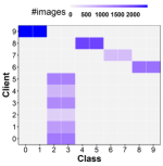
First, most previous studies have focused only on the non-identical distribution aspect, ignoring the non-independent feature of the clients’ data. In reality, the data collected from clients exhibit a substantial degree of clustering, with many clients having similar labels. For example, consider a pill-recognition FL system in which clients use their taken pill images to train the model (as illustrated in Figure 1). Users with the same disease usually have data belonging to identical classes. In other words, clients will be separated into disease-specific categories. In addition, common disease clusters will be considerably larger than other clusters. For example, the users are classified into three groups in Figure 1: diabetic patients, disorder, and others, with the cardinality of the diabetic group being much greater than the disorder group. To fill in this gap, in this work, besides considering common types of non-IID data as existing studies, we focus on a new non-IID data that exhibits non-independent property of data across clients in this work. Specifically, we tackle non-IID data having inter-client correlation, i.e., clients sharing a common feature can have correlated data. We consider that the global distribution of data labels is not uniform, and data labels frequently are partitioned into clusters. The number of clients per group is varied (identified as cluster-skewed non-IID [30, 31]). For cluster-skewed data, utilizing the conventional aggregation strategies, which consider the roles of clients by assigning each client ’s local model a weight depend on the intra-client properties 111 FedAvg [8] and its variance methods assign the weighted based on the number of samples in each clients , i.e., . Methods that enhances training on client side such as FedProx [9] give all the clients a same role with . The approaches optimizing the aggregation adaptively assigned the weights, e.g., based on the client training accuracy and training frequency as in FedFA [10]., will lead to clusters with large numbers of clients dominating the others. To confirm this hypothesis, we have performed a case-study experiment using cluster-skewed data and discovered that in the aggregation process, if we weight clients inversely with the cardinality of the cluster containing them, we can dramatically increase performance compared to vanilla FedAvg (as shown in Figure 2). However, it is crucial to determine how to cluster clients whose dataset is not publicly available. In light of this, we have an important observation that the penultimate layer might provide considerable insights into the training data distribution. Motivated by this fact, we design a novel mechanism to cluster clients based on the data extracted from the penultimate layer of their local models.
Second, the majority of existing approaches either optimize server-side aggregation [10, 20, 21] or enhance client-side training efficiency[9, 25], which results in sub-optimal performance. Therefore, it is crucial to investigate a total solution that simultaneously solves the problem at both the client and server sides. We observe that, in reality, the quantity of data possessed by each client is rather small. In addition, due to the non-IID nature, the data distribution of each client does not correspond to the overall data distribution. Therefore, one of the critical dilemmas is that local model trained on the client side quickly over-fits after several epochs [32, 33]. To tackle this issue, we leverage the Knowledge Distillation paradigm and design a regularization term that aims to narrow the gap between the local and global models, thereby preventing the local model from falling into the local minimum.
Figure 3 depicts the overview of our proposed approach named CADIS (Clustered Aggregation and Knowledge DIStilled Regularization), which consists of four steps: (1) Local training with the aid of KD-based regularization term; (2) Calculating the similarity of clients by utilizing the penultimate layer; (3) Clustering clients into groups; and (4) Aggregating local models using weighted averaging, with the weights determined based on clients’ data size and clusters’ cardinality. Our main contributions are as follows.
-
1.
We perform a theoretical analysis of the penultimate layer to identify its relationship with the training data. Based on the insights retrieved from the penultimate layer, we offer an approach to quantify the similarity between clients, thereby grouping them into clusters.
-
2.
We propose a server-side aggregation approach that adequately handles the cluster-skewed non-IID data. The proposed method is applicable to a wide range of non-IID data problems.
-
3.
We provide a knowledge distillation-based regularization term that overcomes the overfitting in the local training process on the client-side.
-
4.
To demonstrate the superiority of the proposed approach over the state-of-the-art, we conduct comprehensive experiments on the common datasets and our collected real dataset. The results show that our proposal improves the accuracy by up to 16% compared to the FedAvg.
II CADIS - Federated Learning with Clustered Aggregation and Knowledge DIStilled Regularization
The proposed CADIS framework consists of two main components: Cluster-based aggregation on the server and knowledge distillation-based regularization on the client side. Figure 3 shows the overview of our proposed approach named CADIS. In CADIS, the clients utilize SGD to train the model locally using a loss function composed of the cross-entropy loss and a knowledge distillation-based regularization term. Upon receiving the trained models from the clients, the server leverages information collected from the penultimate layer to assess the similarity between the clients. Specifically, the server maintains a so-called Q-matrix that records the clients’ similarities, which are cumulatively updated over communication rounds. Given the similarity of the clients, the server groups them into clusters. Finally, it combines clients’ local models using weighted averaging, where each client’s weight is determined depending on the quantity of its data and the cardinality of its cluster.
In the following, we first give the details of the aggregation process in Section III. We then present the regularization term in Section IV. Section V evaluates the performance of CADIS and compares it to the-state-of-the-art, while the Section VI presents the related works for dealing with different type of non-IID distributions and different approach of cluster-based federated learning. Finally, Section VII concludes the paper.
III Clustered Aggregation

In the following, we first present our proposed cluster-based aggregation formula in Section III-A and then go into the details of our clustering algorithm in Section III-B. Specifically, we introduce an analysis of what the penultimate layer may tell us about the training data distribution in III-B1. Motivated by this finding, we then propose a clustering algorithm based on the improvement of the penultimate layer as shown in Fig. 4. The main idea is to estimate the clients’ data distribution similarity using the improvement of the penultimate layer ( III-B2) and then partition them according to their similarities (III-B3). Moreover, to speed up the convergence of the similarity matrix, we propose a transitive learning mechanism in Section III-C. Finally, we provide an analysis on the rate of our clustered aggregation compared to those of the FedAvg in Section III-D.
III-A Aggregation Formula
Let be the clients. Suppose that () are the clients participating in the training process at the communication round . Upon completion of the local training process, these clients transmit to the server the information of trained local models, denoted by . The server will partition clients into clusters using the algorithm provided in Section III-B. For each client , let be the number of elements of the cluster containing at round . The server then performs weighted aggregation, where client ’s weight, denoted by , is defined as
| (1) |
where is the number of samples owned by client , and is the total samples of all clients. The intuition of this aggregation weight is as follows.
Clients in the same cluster are supposed to have similar training datasets, resulting in similar locally trained models. Let’s consider the following scenario. Suppose cluster has a large number of clients, say fifty, whereas cluster has a small number of clients, say five. Due to the data similarity, the local training at clients in cluster produces fifty similar models, and so do the clients in cluster . To facilitate the understanding, we refer to and as the ones representing the models of clients in cluster and cluster , respectively. If we simply treat all clients equally and aggregate them, then model will have a tenfold greater impact on the global model than model . To equalize the contribution across the clusters, we employ the first term in (1), which is inversely proportional to cluster cardinality. The second term in (1), inherited from FedAvg, is proportional to the number of samples of each client. This term enables clients with more data to contribute more to the global model since clients with more data will, in general, possess more knowledge. Finally, is normalized and applied to the client models’ weights as follows
| (2) |
III-B Penultimate Layer-assisted Clustering Algorithm
III-B1 Insights of the Penultimate Layer
Let us consider a typical deep neural network for a classification task, consisting of a feature extractor and a classifier that is trained using the cross entropy loss by SGD method. We assume that the classifier comprises of a dense layer, represented by , followed by a softmax layer. Here, we give the mathematical supports for the non-bias case because the maths can be easily extended by append a constant to the sample vector . Suppose there are classes, denoted by . We have the following observations.
Proposition III.1.
Suppose , where is the -th row of . Let be a sample with the groundtruth label of , , and be the one-hot vector representing . After training the model with sample , the values of all items in increase while that of the other rows decrease.


Figure 5(a) illustrates an intuition for Proposition III.1. In the upper sub-figure, we trained the model with a sample belonging to class 8 and measured the change of the penultimate layer. It can be observed that the 8-th exhibits positive growth, whereas the remaining rows have negative values.
Sketch Proof. Let denote the representation of . For the sake of the arguments, we assume that all items of are non-negative (attainable with the most popular Sigmoid or ReLU activation functions). Let us denote by the logits of , then is defined as follows
| (3) |
Let be the prediction result which is the output of the softmax layer, then the probability of sample being classified into class , i.e., , is determined by the following formula
| (4) |
The cross entropy loss concerning sample is given by
| (5) |
Let be the item at row and column of , then the gradient of the loss with respect to is
| (6) |
We have
| (7) |
| (8) | ||||
| (9) |
From (7, 8) and (9), we deduce that
| (10) |
As , and (), when applying the gradient descent, the values of the -th row of increase while those on all other rows decrease.
Proposition III.1 can be generalized (with slightly more work) to the case where multiple labels being trained during the training process. Figure 5(a) depicts an illustration for the general case. In the lower sub-figure, we trained the model with samples belonging to classes and . As seen, only the rows may contain positive values, while values of the remaining rows are strictly negative. From this proposition we come up to the following observation.
Observation III.2.
By analyzing the improvement of the penultimate layer, we may identify whether the training data comprises samples from a particular class. Specifically, the training data consists of class ’s samples if and only if the improvement of the -th row of the penultimate layer’s matrix is not negative (i.e., at least one item in the -th row gets higher after training).
Figure 5(b) depicts our observation III.2 in the context of the real-world scenario. Specifically, we train three local models using three pill datasets, two of which contain images of pills taken by diabetic patients and the other by a normal user. The figure demonstrates that the improvement of the penultimate layers of the two diabetic patients is comparable, whereas that of the normal user is clearly different.
III-B2 Similarity Estimation
Let , and be two models locally trained by client and using their respective datasets and . We seek to estimate the similarities of the distributions of and by using the information obtained from the penultimate layers of and . To ease the presentation, in the following, we use the term similarity of client and to indicate the similarity between and ’s data distributions. We encounter the following two significant challenges. First, in the FL training methodology, only a portion of clients engage in the training process during each communication round. Consequently, it is impossible to gather information on the penultimate layers of all clients concurrently. Second, we observe that the change in the penultimate layer throughout each communication round is negligible. It is thus impossible to determine similarity using the raw improvement of the penultimate layer.
To address the first issue, the server will maintain a so-called similarity matrix whose each item depicts the estimated similarity between client and . In each communication round , for each pair of clients participating in that round, the server estimates the instance similarity of and , which depicts the similarity of the training data of and at round . is defined by the following formula
| (11) |
where and are the penultimate layers of and at round , while is the penultimate layer of the global model that the server delivered to the clients at the beginning of round . Note that, and are the improvements of and ’s local models’ penultimate layers after training at round , respectively. Therefore, indicates the cosine similarity between the penultimate layers’ improvements.
As the instance similarity may not accurately reflect the actual similarity between clients, we utilize to update the cumulative similarity in the similarity matrix to achieve accurate estimates. Specifically, is updated as
| (12) |
where represents the total times and have participated in the same communication round up to round .
The second issue, namely the incremental improvement of the penultimate layer, results in the similarity value of all client pairs rapidly converging to .
To this end, our solution is to use the min-max rescaling on the similarity matrix to obtain a so-called -matrix.
III-B3 Client Clustering
Given the -matrix at a communication round , the server uses a binary indicator to determine whether clients and belong to the same cluster as in Equation 13, where is updated upward after every communication round. Note that as is adjusted every round, is also updated over communication rounds, but it will converge after some rounds
| (13) |
III-C Enhancing the Similarity Matrix with Transitive Learning
In the FL training methodology, in each round, there is only a portion of clients participating in the training process. Therefore, it requires significant time for the similarity matrix to converge.
To speedup the convergence, we propose an algorithm to estimate the similarity of two arbitrary clients and via their similarities with other clients.
We notice that cosine similarity possess a transitive characteristic which is reflected by the following theorem [34].
Theorem III.3.
Let denote the cosine similarity of two vectors and . Given three arbitrary vectors and , then their cosine similarities satisfy the following inequality
Motivated by this theorem, we utilize the Gaussian distribution with the mean of and deviation of , denoted as , to estimate the value of . Accordingly, for every client pair which does not co-occurence in a communication round , the server will find all clients such that the deviation of is less than a threshold , i.e., (∗). For each such a client , we denote by a random number following the distribution . The final estimated value for is the average of for all satisfying condition (∗).
Theorem III.4.
Let be the total number of clients and be the number of clients participating in a communication round. Let be the expected number of communication rounds needed to estimate the similarity of all client pairs. Then, .
Sketch Proof. We denote as a random variable representing the number of communication rounds needed for all clients participate in the training at least one time, given clients have already participated in training so far. Then, equals the expected value of , i.e., . can be determined recursively as follows
| (14) |
where is the transitioning probability from state to defined by . We have , and (). Moreover, when , we have (). Therefore, . Accordingly,
It can be deduced that
III-D Convergence Analysis
Finally, we have the following finding on the convergence rate of proposed clustered aggregation compared to FedAvg.
Proposition III.5.
Once converged, the inference loss of the global model achieved by CADIS’s aggregation process is smaller than those generated by FedAvg
| (15) |
where and indicate, respectively, the losses of the converged global models derived by FedAvg and CADIS. Due to space constraints, in the following, we provide a sketch proof when there are clusters among the clients.
Sketch Proof. To simplify, we consider a FL with three clients , in which and belong to a cluster and does not. As loss functions are usually convex ones and have at least one minimum, we consider the simple loss functions for as . Let be the dataset owned by . As and belong to the same cluster, we assume that and are similar. Let be the dataset whose distribution is identical with our targeted data, then can be form by taking a half of , and all of . Accordingly, we can prove that, the optimal loss function when we train a global model with the single set of is given by
| (16) |
Let ( is the number of training epochs) be the trained model that sends to the server at the end of communication round , given the initial model . Then we have
| (17) |
where is the learning rate at the client-side in round .
Aggregation by FegAvg. By aggregaring local models using FegAvg, we obtain the global model as
Aggregation by CADIS. When using CADIS to aggregate the local models, we obtain the following global model
where . When the models converge, we have
By substituting the results above into (16) we obtain
where and ; . By proving and , we deduce that .
IV Knowledge Distillation-based Regularization


We have proposed a clustering strategy to balance the bias on the inter-client level. However, when there are no clusters amongst the clients, the performance of CADIS returns to that of FedAvg, which is sensitive toward intra-client heterogeneity. Therefore, as an extension to our proposal, we integrate a subtle regularization into the local training process to diminish the effect of data heterogeneity. To this end, we design a regularization term inspired by the feature-based knowledge distillation technique [35]. This regularization term intuitively helps the clients to gain new knowledge from their local data without overwriting the previously learnt knowledge in the global model. As a result, the knowledge of the global model is accumulated throughout the federated training process.
We observe that the global model is an aggregation of multiple local models; as a result, it possesses more information and a higher generalizability. Therefore, we use the global model delivered by the server at the beginning of each round as a teacher, while the clients’ local models serve as students. A client’s regularization term is then defined by the Kullback-Leibler (KL) divergence between the representations generated by the client’s local model and those obtained from the global model. Figure 7 illustrates the flow for a client calculate the regularization term. The details are as follows. Consider a client with the training dataset of , let be the representations generated by the locally trained model, and be the representation produced by global model delivered by the server. Instead of model the distribution of and directly, we try to model the pairwise interactions between their data samples, because as helps to describe the geometry of their respective feature spaces [36]. To accomplish this, we employ the joint probability density, which represents the likelihood that two data points are close together. These joint density probability functions can be easily estimated using Kernel Density Estimation (KDE) [37]. Let and be the joint density probability functions corresponding to and . Suppose denote the joint probability of and then can be estimated using KDE as , where is a Gaussian kernel, with is the bandwidth of the Gaussian bell. However, as stated in [38], it is often impossible to learn a model that can accurately reproduce the entire geometry of a complex teacher model. Therefore, the conditional probability distribution of the samples can be used instead of the joint probability density function as follows
| (18) |
The similar process is applied to estimate the probability distribution of the global model. Finally, we use Kullback-Leibler (KL) divergence to calculate the difference between the two distributions and by using the following formula
| (19) |
where is the batch size. Consequently, the final loss function for training at client in round is defined as
| (20) |
Here is the cardinality of ’s dataset, is the number of training epochs; is training dataset of the -th batch, where depicts the image set, and denotes the corresponding labels; is the weighting factor of the regularization term.
V Experiments and Results
This section evaluates the performance of the proposed FL method, i.e., CADIS, against competing approaches for various FL scenarios. We show that CADIS is able to achieve higher performance and more stable convergence compared with state-of-the-art FL methods including FedAvg [8], FedProx [9], FedDyn [25], and FedFA [39], on various datasets and non-IID settings. In the following, we first introduce four image classification datasets used in our experiments including both standard conventional datasets and real-world medical imaging datasets. We also describe the setup for the experiments in Section V-A. We then report and compare the performance of the CADIS with state-of-the-art methods using the top-1 accuracy on the test datasets. (Section V-B). In all experiments, the SingleSet setting (centralized training at the server or training in the system of only one client)222Because Singleset trained on a single client (or server), it may be equivalent to training with an IID dataset. is used as the reference. Finally, in Section V-C, we conduct ablation studies to highlight some key properties of CADIS.
V-A Datasets and Experimental Settings
To evaluate the robustness of the proposed method in a real-world setting, we collect a large-scale real-world pill image classification dataset (due to the double-blind policy, we name our dataset as PILL). The dataset consists in total of images from patients, diagnoses and pills (classes). However, in our experiments, we use a subset of clients constituted clients diagnosed with diabetes and clients from other diseases. We then annotate the data of selected clients to be our evaluated sub-dataset 333We have to evaluate on sub-dataset because of the lack of manpower to annotate the whole dataset at the time of submission.. The sub-dataset consists of classes, e.g., the pill name, and images. The dataset is then divided into two disjoint parts, where % of images are used for training and the rest % are used for testing.
To further evaluate the effectiveness of CADIS on bigger datasets, we use three benchmark imaging datasets with the same train/test sets as in previous work [8, 9, 25, 39], which are MNIST [40], CIFAR-10 [41], and CIFAR-100 [41]. We simulate data heterogeneity scenarios, i.e., cluster-skewed non-IID, by partitioning datasets and distributing the training samples among clients. In this work, we target the sample-unbalanced multi-cluster (denoted as MC) non-IID, in which clients have the same label distribution belonging to the same cluster. We choose clusters with the ratio of clients in the clusters are . The number of samples per client is unbalanced and each client has approximately of labels (classes), e.g., 2 classes for CIFAR-10. We also further consider different data partition methods in SectionV-C. Figure 7 illustrates the class distribution of the PILL subset and CIFAR-10 dataset across clients with MC partition methods.
We train simple convolutional neural networks (CNNs) on MNIST as mentioned in [8]. Specifically, we train ResNet-9 [42] network on CIFAR-10, and CIFAR-100 dataset, and ResNet-18 [42] on PILL dataset. For all the experiments, we use SGD (stochastic gradient descent) as the local optimizer. We also set the local epochs , a learning rate of , and a local batch size . We evaluate with the system of 100 clients like prior work in FL [8, 9]. The number of participating clients at each communication round is for PILL and for other datasets. We also used the default hyper-parameters suggested by the original paper of each FL benchmark. Specifically, we set the proximal term for the FedProx method. For FedFA, we set and as suggested in [39]. For FedDyn, we use [25].
V-B Experimental Results
| Dataset | #Clients | Top-1 Accuracy (%) | Impr. (%) | ||||||
| SingeSet | FedAvg | FedProx | FedFA | FedDyn | CADIS | (a) | (b) | ||
| PILL | 3/10 | 92.32 | 73.36 | 70.04 | 6.67 | 22.17 | 79.71 | 8.7 | 8.7 |
| CIFAR-10 | 10/100 | 82.11 | 48.74 | 48.43 | 10.00 | 19.62 | 50.09 | 2.8 | 2.8 |
| CIFAR-100 | 10/100 | 52.36 | 33.42 | 33.21 | 36.49 | 5.39 | 38.09 | 14.0 | 4.4 |
| 20/100 | 52.36 | 32.70 | 32.13 | 35.28 | 3.68 | 38.16 | 16.7 | 8.2 | |
| 30/100 | 52.36 | 32.07 | 32.37 | 35.42 | 5.73 | 38.55 | 20.2 | 8.8 | |
| 40/100 | 52.36 | 31.65 | 31.48 | 35.20 | 6.30 | 36.35 | 14.8 | 3.3 | |
| 50/100 | 52.36 | 31.11 | 31.27 | 35.12 | 6.59 | 36.23 | 16.5 | 3.2 | |
| MNIST | 10/100 | 99.15 | 93.04 | 92.91 | 93.33 | 88.04 | 93.45 | 0.4 | 0.1 |
| 20/100 | 99.15 | 95.12 | 95.12 | 95.55 | 93.58 | 95.71 | 0.6 | 0.2 | |
| 30/100 | 99.15 | 95.06 | 95.02 | 95.50 | 93.92 | 96.00 | 1.0 | 0.5 | |
| 40/100 | 99.13 | 94.10 | 94.05 | 94.50 | 88.04 | 95.60 | 1.6 | 1.2 | |
| 50/100 | 99.15 | 94.83 | 94.86 | 95.27 | 93.55 | 96.20 | 1.4 | 1.0 | |
-
•
(*) The best and second best results are highlighted in the bold-red and bold-blue.
(**) impr.(a) and impr.(b) are the relative accuracy improvement of CADIS compared with FedAvg and the best benchmark FL method (in percentage), respectively.
V-B1 Top-1 accuracy
Table I presents the results of the classification accuracy when comparing our proposed CADIS to the baseline methods on all the datasets with cluster-skewed non-IID. We report the best accuracy that each FL method reaches within communication rounds. Specifically, CADIS achieves better accuracy than all other FL methods. For example, CADIS achieves an accuracy of % on the PILL dataset. This result significantly outperforms the best benchmark FL methods, e.g., FedAvg, by %. Compared to the second-best benchmark (marked in bold-blue text), our CADIS surpasses it by %, %, and % top-1 accuracy in CIFAR-10, CIFAR-100, and MNIST datasets, respectively ( clients participating in each round). It is worth noting that the image classification tasks in MNIST dataset are simple such as the accuracy of all the methods is asymptotic to that of the SingleSet, leading no room for optimizing. As a result, CADIS is only slightly better than the baseline methods. This result emphasizes that our cluster-based weighted aggregation method can engage the clients from the ‘smaller’ clusters (i.e., groups with a smaller cardinality) more effectively than the sample-quantity-based aggregation of FedAvg and the training-frequency-based aggregation of FedFA. It demonstrates our theoretical finding mentioned in Proposition III.5.
We next conduct a sensitivity study to quantify the impact of the number of participating clients per communication round on accuracy. As shown in Table I, we change from up to when training on the CIFAR-100 and MNIST datasets. We observe that varying the number of participating clients would slightly affect the top-1 accuracy but would not impact the relative result between CADIS and the baseline methods. As the result, the improvement in accuracy of CADIS over the other two baseline methods is consistently maintained.
V-B2 Convergence analysis


To demonstrate the effectiveness of CADIS in reducing local computation at clients, we provide the number of communication rounds to reach a target top-1 accuracy and speedup relative to the FedAvg (Table II. Overall, the convergence rate of CADIS is fastest in most of the evaluated cases except for the CIFAR-100 dataset. Specifically, to reach an accuracy of % for the PILL dataset, CADIS requires only communication rounds. FedAvg and FedProx spend longer than CADIS. In addition, CADIS is equivalent to FedFA in the case of MNIST dataset, while it is slower than FedFA in the case of CIFAR-100. It is because CADIS requires some first communication rounds for the similarity matrix coverage (Theorem III.4), which leads to an incorrect clustering and slow down its coveragence rate. However, it is worth noting that CADIS achieves higher top-1 accuracy than FedFA when converged.
| Dataset | Acc. | FedAvg | FedProx | FedFA | FedDyn | CADIS |
|---|---|---|---|---|---|---|
| PILL | 60% | 74 | 74 (1.0) | N/A | N/A | 45 (1.6) |
| 70% | 159 | 338 (0.5) | N/A | N/A | 136 (1.2) | |
| MNIST | 80% | 94 | 94 (1.0) | 94 (1.0) | 279 (0.3) | 94 (1.0) |
| 90% | 341 | 341 (1.0) | 281 (1.2) | N/A | 281 (1.2) | |
| CIFAR-10 | 48% | 960 | 960 (1.0) | N/A | N/A | 537 (1.8) |
| CIFAR-100 | 35% | N/A | N/A | 281 | N/A | 644 |
-
•
(*) The symbol N/A means the method is not able to reach the target test accuracy.
V-C Ablation studies
V-C1 Robustness to the client datasets
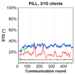
In the previous subsection, we focus on the top-1 testing accuracy on an IID test dataset to estimate the goodness of the trained model over the global distribution. Because only a small portion of clients participate in the training process at each communication round, the aggregated global model at the server overly fits the sub-dataset of some clients, e.g., most-recently trained clients, or clients in the same cluster. To estimate the robustness of an FL method against clients, we consider the trend of top-1 accuracy by estimating the average accuracy obtained in the last communication rounds (named -round averaging accuracy for short). As shown in Figure 8(a) (Left), the difference in the top-1 accuracy between two communication rounds of FedAvg and FedProx is non-trivial. The top-1 accuracy of CADIS oscillates with a smaller amplitude than those of FedAvg and FedProx. As the result, there is a clear gap of -round averaging accuracy between CADIS and the FedAvg as shown in Figure 8(a) (Middle). Another interesting point is that although CADIS is equivalent to another baseline method for the MNIST dataset in terms of top-1 accuracy, the -round averaging accuracy of CADIS outperforms those of the baseline significantly, e.g., % as in CADIS versus around % of FedAvg (Figure 8(a) (Right). We also test the global model on the local sub-dataset of all the participating clients at the beginning of each communication round, i.e., do the inference pass at clients. The result in Figure 8(b) shows that CADIS has consistently higher average inference accuracy across clients with smaller variances than the baselines.
The results imply that the aggregated global model obtained by CADIS is more stable than the others and does not overfit clients’ sub-datasets. It is expected because CADIS is designed with Knowledge Distillation-based Regularization for clients to avoid the local overfitting issue. Thus, we state that our CADIS could learn a well-balanced model between clients.
V-C2 Impact of the non-IID type
| Partitioning method | MNIST | CIFAR-10 | CIFAR-100 | ||||||
|---|---|---|---|---|---|---|---|---|---|
| PA | BC | UC | PA | BC | UC | PA | BC | UC | |
| SingeSet | 99.22 | 99.24 | 99.18 | 81.37 | 39.20 | 84.75 | 80.85 | 52.66 | 52.62 |
| FedAvg | 96.89 | 96.69 | 96.02 | 62.26 | 20.22 | 43.45 | 21.01 | 34.96 | 34.16 |
| FedProx | 96.73 | 96.66 | 96.01 | 62.63 | 20.18 | 43.86 | 20.76 | 34.61 | 34.06 |
| FedFA | 96.50 | 96.67 | 96.29 | 66.41 | 10.00 | 10.00 | 1.00 | 37.18 | 37.38 |
| FedDyn | 92.79 | 93.36 | 91.72 | 18.79 | 19.34 | 19.28 | 2.14 | 9.69 | 13.75 |
| CADIS | 96.89 | 96.74 | 96.58 | 62.93 | 34.83 | 47.42 | 21.52 | 34.96 | 34.62 |
-
•
(*) The best and second best results are highlighted in the red and blue.
We study the robustness of our method with the different types of non-IID by considering both conventional label distribution skew (Pareto), and other patterns of cluster skew [31] ( and ).
- •
-
•
Sample-balanced single cluster (denoted as BC): a simple case of cluster skew with only one cluster and the number of samples per client does not change among clients. To measure the bias of the proposed model toward the cluster, we choose the number of clients inside the cluster significantly higher than the others, e.g, 60%.
-
•
Sample-unbalanced single cluster (denoted as UC): Similar to the BC but the number of samples per client is unbalanced.
In Section V-B, we showed numerical data regarding the MC distribution, in which CADIS demonstrated an improvement in accuracy compared to other methods. A similar observation was observed in the PA, BC, and UC data distribution (Table III). CADIS achieves the best top-1 accuracy in most of the experiments (the second-best top-1 in the remaining). For example, CADIS improves the top-1 accuracy by and in the case of the CIFAR-10 dataset, BC and UC, respectively. The result implies that CADIS has a good performance with different types of cluster-skewed non-IID while achieving acceptable performance with label distribution non-IID (equivalent to FedAvg).
V-D Discussion
V-D1 Impact of the transitive learning


We introduced transitive learning in Section III-C to speed up the convergence of the similarity matrix. We confirm that CADIS with transitive learning (Transitive) and without transitive learning (Standard) could reach the same accuracy in our experiment. However, transitive learning clusters the clients into groups faster than Standard. Figure 10 shows the MSE distance of the similarity matrix built up by two methods with the correct similarity matrix (ideal one). Transitive could coverage after communication rounds while Standard needs approximate rounds.
V-D2 Impact of hyper-parameters
In the experiments shown in Section V-B, we tune the similarity threshold and the factor and report the best result obtained. In this section, we discuss how the hyper-parameters impact the top-1 accuracy. Figure 10 show the results when we change both hyper-parameters of CADIS on the CIFAR-100 dataset, MC distribution. The result shows that both two hyper-parameter could lead to a change in accuracy. However, CADIS is much more sensitive to the similarity threshold . For example, CADIS[, ] achieve % while CADIS[, ] reaches %. In our experiment, the best similarity threshold also changes when we change the dataset, e.g., for MNIST and for CIFAR-10 and CIFAR-100.
V-D3 The generalization of proposition III.1
It is worth noting that the proof of proposition III.1 can be used regardless of the condition . In the case where the values of are not confined to the non-negative domain, one may deduce that the updates among rows of the penultimate layer will exhibit an inverse trend, depending on the label being trained. However, since our objective is to discover the labels underlying the training dataset, we only analyze the scenario in which the representation vector is monotonically non-negative.
V-D4 Computational Overhead
We now estimate the computational overhead of the aggregation at the server of CADIS in comparison with FedAvg and the other methods. The result in Fig. 11 (Left) shows that the computation overhead at the server of the CADIS’s clustering module is trivial, i.e., the time of CADIS is approximate those of FedAvg and FedProx. This is an expected result because CADIS clusters the clients based on the information of the penultimate layer whose size is quite small, e.g., in the case of the ResNet-9 model and CIFAR-100 dataset.
For the computation overhead of local training at client, we estimate the relative performance (on average) of CADIS over those one of FedAvg using the same device setting, e.g., the GPU Force-GTX 3090. The result in Fig. 11 (Right) shows CADIS require more computation at local than FedAvg (for performing the knowledge distillation regularization).

VI Related Works
To tackle the statistical heterogeneity, i.e., non-IID, problem, many efforts focused on designing weighting strategies for aggregation at server [10, 20, 21]. The authors in [10] developed a weighed aggregation mechanism, in which the weight of a client’s local model is the sum of the information entropy calculated from the accuracy of the local model and the number of the client has participated in the training. In [20], Wang et al., focused on the internal and externa conflict between the clients. The former indicates the unfairness among clients selected in the same round, whereas the latter represents a conflict between the assumed gradient of a client who has not been chosen and the global update. In order to accomplish this, they proposed a mechanism to eliminate conflicts before averaging the gradients. Alternatively, many studies improve the training algorithm at client side [9, 25, 26, 27]. In [9], the authors addressed data heterogeneity by adding a so-called proximal term to the loss function, which restricts local updates to be closer to the initial (global) model. The authors in [25] used an adaptive regularization term leveraging the cumulative gradients when training the local models. In [26], the authors investigated how to remedy the client drift induced by the heterogeneous data among clients in their local updates.
However, previous studies specifically take into account the label skew non-IID when each client has a fixed number of classes (label size imbalance [8, 9, 43, 28, 44, 45]) or when the number of samples of a certain class is distributed to clients using the power-law or Dirichlet distribution (label distribution imbalance [13, 46, 39, 27]). Recently, some works consider the non-IID scenario which is more close to the real-world data such as the numbers of classes are often highly imbalanced [29], or following the cluster-skew non-IID distribution [30, 31]. Especially, cluster-skew is firstly introduced by [30] where there exists a data correlation between clients. Authors in [31] tackle this data distribution by adaptively assigning the weights for clients at aggregation by using Deep Reinforcement Learning. This work also focuses on cluster-skew. Unlike [31], we combine both the aggregation optimization approach (clustered aggregation) at the server side and the training enhancement approach at clients (knowledge distillation-based regularization) in this work.
Cluster-based Federated Learning: Recent works cluster the clients into groups where different groups of clients have different learning tasks [47, 48], or different computation/network resource [43, 49]. Other methods have been proposed to identify adversarial clients and remove them from the aggregation [50, 48] based on their cosine similarities. Recently [51, 52] proposed to use clustering to address the non-IID issue. It is worth noting that most of the previous cluster-based Federated Learning methods assume that all clients will participate in the clustering process or use the whole model for clustering which is unpractical in a real Federated Learning system. Our proposed CADIS can effectively cluster clients by using the information of the penultimate layer only.
VII Conclusion
In this paper, we introduced for the first time a new type of non-IID data called cluster-skewed non-IID, in which clients can be grouped into distinct clusters with similar data distributions. We then provided a metric that quantifies the similarity between two clients’ data distributions without violating their privacy, and then employed a novel aggregation scheme that guarantees equality between clusters. Moreover, we designed a local training regularization based on the knowledge-distillation technique that reduces the impact of overfitting on the clients’ training process and dramatically boosts the trained model’s performance. We performed the theoretical analysis to give the basis of our proposal and proved its superiority against a benchmark. Extensive experimental results on both standard public datasets and our own collected real pill image dataset demonstrated that our proposed method, CADIS, outperforms state-of-the-art. Notably, in the cluster-skewed scenario, our proposed FL framework, CADIS, improved top-1 accuracy by % compared to FegAvg and by up to % concerning other state-of-the-art approaches.
VIII Acknowledgments
This work was funded by Vingroup Joint Stock Company (Vingroup JSC),Vingroup, and supported by Vingroup Innovation Foundation (VINIF) under project code VINIF.2021.DA00128. This work was supported by JSPS KAKENHI under Grant Number JP21K17751 and is based on results obtained from a project, JPNP20006, commissioned by the New Energy and Industrial Technology Development Organization (NEDO).
References
- [1] M. Chiang and T. Zhang, “Fog and iot: An overview of research opportunities,” IEEE Internet of Things Journal, vol. 3, no. 6, pp. 854–864, 2016.
- [2] N. Abbas, Y. Zhang, A. Taherkordi, and T. Skeie, “Mobile edge computing: A survey,” IEEE Internet of Things Journal, vol. 5, no. 1, pp. 450–465, 2018.
- [3] H. Li, K. Ota, and M. Dong, “Learning iot in edge: Deep learning for the internet of things with edge computing,” IEEE Network, vol. 32, no. 1, pp. 96–101, 2018.
- [4] Y. Wei and M. B. Blake, “Service-oriented computing and cloud computing: Challenges and opportunities,” IEEE Internet Computing, vol. 14, no. 6, pp. 72–75, 2010.
- [5] H. Takabi, J. B. Joshi, and G.-J. Ahn, “Security and privacy challenges in cloud computing environments,” IEEE Security and Privacy, vol. 8, no. 6, pp. 24–31, 2010.
- [6] J. Domingo-Ferrer, O. Farràs, J. Ribes-González, and D. Sánchez, “Privacy-preserving cloud computing on sensitive data: A survey of methods, products and challenges,” Computer Communications, vol. 140-141, pp. 38–60, 2019.
- [7] M. B. Mollah, M. A. K. Azad, and A. Vasilakos, “Security and privacy challenges in mobile cloud computing: Survey and way ahead,” Journal of Network and Computer Applications, vol. 84, pp. 38–54, 2017.
- [8] B. McMahan, E. Moore et al., “Communication-efficient learning of deep networks from decentralized data,” in Artificial Intelligence and Statistics. PMLR, 2017, pp. 1273–1282.
- [9] T. Li, A. K. Sahu et al., “Federated optimization in heterogeneous networks,” Proceedings of Machine Learning and Systems, vol. 2, pp. 429–450, 2020.
- [10] W. Huang, T. Li, D. Wang, S. Du, J. Zhang, and T. Huang, “Fairness and accuracy in horizontal federated learning,” Information Sciences, vol. 589, pp. 170–185, 2022.
- [11] X. Ma, J. Zhu, Z. Lin, S. Chen, and Y. Qin, “A state-of-the-art survey on solving non-iid data in federated learning,” Future Generation Computer Systems, vol. 135, pp. 244–258, 2022.
- [12] H. Zhu, J. Xu et al., “Federated learning on Non-IID data: A survey,” arXiv preprint arXiv:2106.06843, 2021.
- [13] X. Li, K. Huang, W. Yang, S. Wang, and Z. Zhang, “On the convergence of FedAvg on Non-IID data,” in 8th International Conference on Learning Representations, ICLR 2020, Addis Ababa, Ethiopia, April 26-30, 2020, 2020.
- [14] T. Li, A. K. Sahu, A. Talwalkar, and V. Smith, “Federated learning: Challenges, methods, and future directions,” IEEE Signal Processing Magazine, vol. 37, no. 3, pp. 50–60, 2020.
- [15] H. Wang, Z. Kaplan, D. Niu, and B. Li, “Optimizing federated learning on non-iid data with reinforcement learning,” in IEEE INFOCOM 2020 - IEEE Conference on Computer Communications, 2020, pp. 1698–1707.
- [16] J. Zhang, S. Guo, Z. Qu, D. Zeng, Y. Zhan, Q. Liu, and R. Akerkar, “Adaptive federated learning on non-iid data with resource constraint,” IEEE Transactions on Computers, vol. 71, no. 7, pp. 1655–1667, 2022.
- [17] F. Hu, W. Zhou, K. Liao, and H. Li, “Contribution- and participation-based federated learning on non-iid data,” IEEE Intelligent Systems, pp. 1–1, 2022.
- [18] M. Jiang, Z. Wang, and Q. Dou, “Harmofl: Harmonizing local and global drifts in federated learning on heterogeneous medical images,” in Proceedings of the AAAI Conference on Artificial Intelligence, vol. 36, no. 1, 2022, pp. 1087–1095.
- [19] J. Zhang, S. Guo, Z. Qu, D. Zeng, Y. Zhan, Q. Liu, and R. Akerkar, “Adaptive federated learning on non-iid data with resource constraint,” IEEE Transactions on Computers, vol. 71, no. 7, pp. 1655–1667, 2021.
- [20] Z. Wang, X. Fan, J. Qi, C. Wen, C. Wang, and R. Yu, “Federated learning with fair averaging,” 2021 International Joint Conference on Artificial Intelligence (IJCAI), 2021.
- [21] H. Wu and P. Wang, “Fast-convergent federated learning with adaptive weighting,” IEEE Transactions on Cognitive Communications and Networking, vol. 7, no. 4, pp. 1078–1088, 2021.
- [22] Y. J. Cho, J. Wang et al., “Client selection in federated learning: Convergence analysis and power-of-choice selection strategies,” arXiv preprint arXiv:2010.01243, 2020.
- [23] H. Wang, Z. Kaplan et al., “Optimizing federated learning on non-IID data with reinforcement learning,” in IEEE Conference on Computer Communications (INFOCOM), 2020, pp. 1698–1707.
- [24] D. Y. Zhang, Z. Kou, and D. Wang, “FedSens: A federated learning approach for smart health sensing with class imbalance in resource constrained edge computing,” in IEEE Conference on Computer Communications (INFOCOM 2021), 2021, pp. 1–10.
- [25] D. A. E. Acar, Y. Zhao, R. Matas, M. Mattina, P. Whatmough, and V. Saligrama, “Federated learning based on dynamic regularization,” in International Conference on Learning Representations, 2021. [Online]. Available: https://openreview.net/forum?id=B7v4QMR6Z9w
- [26] S. P. Karimireddy, S. Kale, M. Mohri, S. Reddi, S. Stich, and A. T. Suresh, “Scaffold: Stochastic controlled averaging for federated learning,” in International Conference on Machine Learning. PMLR, 2020, pp. 5132–5143.
- [27] J. Wang, Q. Liu et al., “A novel framework for the analysis and design of heterogeneous federated learning,” IEEE Transactions on Signal Processing, vol. 69, pp. 5234–5249, 2021.
- [28] H. Zeng, T. Zhou, Y. Guo, Z. Cai, and F. Liu, FedCav: Contribution-aware model aggregation on distributed heterogeneous data in federated learning. New York, NY, USA: Association for Computing Machinery, 2021.
- [29] X. Shuai, Y. Shen, S. Jiang, Z. Zhao, Z. Yan, and G. Xing, “Balancefl: Addressing class imbalance in long-tail federated learning,” in 2022 21st ACM/IEEE International Conference on Information Processing in Sensor Networks (IPSN), 2022, pp. 271–284.
- [30] K. Hsieh, A. Phanishayee et al., “The non-IID data quagmire of decentralized machine learning,” in Proceedings of the 37th International Conference on Machine Learning (ICML), vol. 119. PMLR, 13–18 Jul 2020, pp. 4387–4398.
- [31] N. H. Nguyen, P. L. Nguyen, D. L. Nguyen, T. T. Nguyen, T. D. Nguyen, H. H. Pham, and T. T. Nguyen, “FedDRL: Deep Reinforcement Learning-based Adaptive Aggregation for Non-IID Data in Federated Learning,” 2022. [Online]. Available: https://arxiv.org/abs/2208.02442
- [32] S. Ji, T. Saravirta, S. Pan, G. Long, and A. Walid, “Emerging trends in federated learning: From model fusion to federated x learning,” 2021. [Online]. Available: https://arxiv.org/abs/2102.12920
- [33] M. Mohri, G. Sivek, and A. T. Suresh, “Agnostic federated learning,” in Proceedings of the 36th International Conference on Machine Learning, ser. Proceedings of Machine Learning Research, K. Chaudhuri and R. Salakhutdinov, Eds., vol. 97. PMLR, 09–15 Jun 2019, pp. 4615–4625.
- [34] E. Schubert, “A triangle inequality for cosine similarity,” in International Conference on Similarity Search and Applications. Springer, 2021, pp. 32–44.
- [35] N. Passalis and A. Tefas, “Learning deep representations with probabilistic knowledge transfer,” in Proceedings of the European Conference on Computer Vision (ECCV), September 2018.
- [36] L. Van der Maaten and G. Hinton, “Visualizing data using t-sne.” Journal of machine learning research, vol. 9, no. 11, 2008.
- [37] D. W. Scott, Multivariate density estimation: theory, practice, and visualization. John Wiley & Sons, 2015.
- [38] N. Passalis and A. Tefas, “Learning deep representations with probabilistic knowledge transfer,” in Proceedings of the European Conference on Computer Vision (ECCV), 2018, pp. 268–284.
- [39] W. Huang, T. Li et al., “Fairness and accuracy in federated learning,” arXiv preprint arXiv:2012.10069, 2020.
- [40] Y. Lecun, L. Bottou et al., “Gradient-based learning applied to document recognition,” Proceedings of the IEEE, vol. 86, no. 11, pp. 2278–2324, 1998.
- [41] A. Krizhevsky and G. Hinton, “Learning multiple layers of features from tiny images,” Master’s thesis, Dep. of Comp. Sci. Univ. of Toronto, 2009.
- [42] K. He, X. Zhang, S. Ren, and J. Sun, “Deep residual learning for image recognition,” in CVPR, 2016, pp. 770–778.
- [43] Z. Chai, Y. Chen et al., “FedAT: A high-performance and communication-efficient federated learning system with asynchronous tiers,” in Proceedings of the International Conference for High Performance Computing, Networking, Storage and Analysis, ser. SC ’21, 2021.
- [44] Z. Wang, X. Fan et al., “Federated learning with fair averaging,” in Proceedings of the Thirtieth International Joint Conference on Artificial Intelligence, IJCAI-21, Z.-H. Zhou, Ed. International Joint Conferences on Artificial Intelligence Organization, 8 2021, pp. 1615–1623.
- [45] P. Xiao, S. Cheng et al., “Averaging is probably not the optimum way of aggregating parameters in federated learning,” Entropy, vol. 22, no. 3, p. 314, 2020.
- [46] Z. Wang, Y. Zhu et al., “FedACS: Federated skewness analytics in heterogeneous decentralized data environments,” in IEEE/ACM 29th International Symposium on Quality of Service (IWQOS), 2021, pp. 1–10.
- [47] A. Ghosh, J. Chung, D. Yin, and K. Ramchandran, “An efficient framework for clustered federated learning,” in Advances in Neural Information Processing Systems, H. Larochelle, M. Ranzato, R. Hadsell, M. Balcan, and H. Lin, Eds., vol. 33. Curran Associates, Inc., 2020, pp. 19 586–19 597.
- [48] F. Sattler, K.-R. Müller, and W. Samek, “Clustered federated learning: Model-agnostic distributed multitask optimization under privacy constraints,” IEEE Transactions on Neural Networks and Learning Systems, vol. 32, no. 8, pp. 3710–3722, 2021.
- [49] K. Muhammad, Q. Wang, D. O’Reilly-Morgan, E. Tragos, B. Smyth, N. Hurley, J. Geraci, and A. Lawlor, “Fedfast: Going beyond average for faster training of federated recommender systems,” in Proceedings of the 26th ACM SIGKDD International Conference on Knowledge Discovery and Data Mining, ser. KDD ’20. New York, NY, USA: Association for Computing Machinery, 2020, p. 1234–1242.
- [50] F. Sattler, K.-R. Müller, T. Wiegand, and W. Samek, “On the byzantine robustness of clustered federated learning,” in ICASSP 2020 - 2020 IEEE International Conference on Acoustics, Speech and Signal Processing (ICASSP), 2020, pp. 8861–8865.
- [51] C. Chen, Z. Chen, Y. Zhou, and B. Kailkhura, “Fedcluster: Boosting the convergence of federated learning via cluster-cycling,” in 2020 IEEE International Conference on Big Data (Big Data), 2020, pp. 5017–5026.
- [52] C. Briggs, Z. Fan, and P. Andras, “Federated learning with hierarchical clustering of local updates to improve training on non-iid data,” in 2020 International Joint Conference on Neural Networks (IJCNN). IEEE, 2020, pp. 1–9.
- [53] Z. Wang, X. Fan, J. Qi, C. Wen, C. Wang, and R. Yu, “Federated learning with fair averaging,” arXiv preprint arXiv:2104.14937, 2021.
Appendix A Artifact Description
BADGE APPLICATION: Open Research Objects (ORO)
A-A SUMMARY OF EXPERIMENTAL SETTINGS
Our codes has been published at Artifact 1, which is a modified framework for federated learning introduced in [53]. The original framework can be accessed at Artifact 2. To reproduce our experiments, simply follow the instructions shown in the Readme file. Below are detailed experimental and hyperparameter settings.
At clients, we apply Stochastic Gradient Descent (SGD) as the optimizer with the learning rate , batch size and local epochs if not explicitly say otherwise. The knowledge distillation-based loss is scaled with the factor , which is set during experiments, if not explicitly say otherwise. The number of total clients varies from to whereas the participation ratio every round increases from to . Regarding the server, the similarity-based clustering threshold is varied regarding different datasets. In details, we found that worked best for MNIST, for CIFAR10 and CIFAR100.
A-B HARDWARE
Most of experiments were conducted on a computer that consists of 2 Intel Xeon Gold CPUs, and 4 NVIDIA V100 GPUs. We deploy only one experiment on an entire GPU. For the computation overhead of local training at client, we estimate the relative performance (on average) of CADIS over those one of FedAvg using the same device setting, e.g., the GPU Force-GTX 3090.
Note that some of our experiments are intensive. With aforementioned system, an experiment takes up to 36 hours to complete. Therefore, low-resource systems might take few days. We highly recommend a system that is equal to or better than aforementioned settings for experimental reproducibility.
A-C SOFTWARE
We use a pytorch-implemented framework for experimental evaluation. Whilst the full requirement can be viewed in the README.md in Artifact 1, below are some prerequisites:
-
•
Compilers: Python 3.8.12
-
•
Frameworks: Pytorch - py3.8_cuda11.3_cudnn8.2.0_0
-
•
Support libraries: wandb 0.13.5
-
•
Core libraries: please check README.md
-
•
Datasets: CIAFR-10, MNIST, CIFAR-100.
A-D ARTIFACTS
Artifact 1
Github: ORO-CCGRID2023-CADIS
Artifact name: ORO-CCGRID2023-CADIS
Artifact 2
Github: easyFL
Artifact name: easyFL