BézierFormer: A Unified Architecture for 2D and 3D Lane Detection
Abstract
Lane detection have made significant progress in recent years, but there is not a unified architecture for its two sub-tasks: 2D lane detection and 3D lane detection. To fill this gap, we introduce BézierFormer, a unified 2D and 3D lane detection architecture based on Bézier curve lane representation. BézierFormer formulate queries as Bézier control points and incorporate a novel Bézier curve attention mechanism. This attention mechanism enables comprehensive and accurate feature extraction for slender lane curves via sampling and fusing multiple reference points on each curve. In addition, we propose a novel Chamfer IoU-based loss which is more suitable for the Bézier control points regression. The state-of-the-art performance of BézierFormer on widely-used 2D and 3D lane detection benchmarks verifies its effectiveness and suggests the worthiness of further exploration.
Index Terms:
2D Lane Detection, 3D Lane Detection, Autonomous Driving, Bézier CurveI Introduction
Lane detection based on RGB images is a critical foundational perception task in various applications such as autonomous driving, lane-level AR navigation, and HD map construction. This task is specifically divided into 2D lane detection and 3D lane detection. Both of them are challenging due to the inherent difficulties, including obscured or worn lane markers, and variations in lighting and weather conditions. With the advent of deep learning, both 2D and 3D lane detection have made significant progress [1, 2, 3, 4, 5, 6, 7, 8]. However, there is not a unified architecture for these two subtasks, although they share many similarities. It usually takes a lot of efforts to adapt a state-of-the-art 2D lane detection model to 3D lane detection(or vice versa), and this hinders further development of lane detection. In this paper, we aim to answer the question of whether it is possible to build a unified state-of-the-art architecture for both 2D and 3D lane detection.
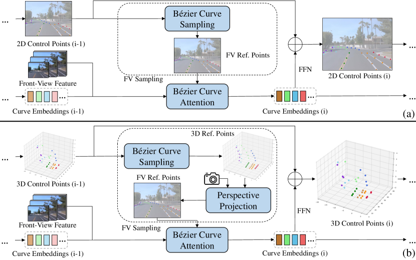
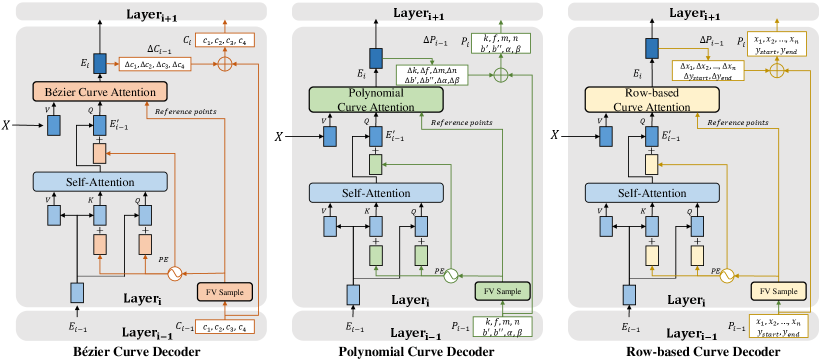
First of all, we utilize the Bézier curve to represent lane curves in our method, because Bézier curve can uniformly and efficiently represent both 2D and 3D curves via a few control points. Inspired by the DEtection TRansformers [9, 10], we introduce BézierFormer, which aims to query lane features from the input monocular image and output 2D or 3D control points of lanes. As shown in Figure 1, our method formulates queries as dynamic Bézier control points, uses a Bézier curve attention mechanism to extract lane features. Besides we propose a Chamfer IoU-based loss compatible with 2D and 3D Bézier control points regression.
Specifically, initial control point queries, learnable curve embeddings, and image features are fed into the decoder. With the aid of Bézier curve attention, each decoder layer extracts lane features accurately and comprehensively to refine curve embeddings and control points from the previous layer. To implement Bézier curve attention mechanism, the front-view (FV) sampling module first samples a few sparse reference points along the curve based on control points, ensuring that the attention’s receptive field fully covers the entire lane curve. Then we use the Bézier curve attention operation, a multi-reference-points variant of deformable attention [11], to extract and fuse the features around these reference points on the curve. Finally, extracted lane features enhance curve embeddings for lane regression and recognition. For lane regression, we present a loss derived from Chamfer Distance. It facilitates a more effective learning process by fitting the overall shape of the target curve. To make our method compatible with 2D and 3D lane detection, there is an optional perspective projection operation in the FV sampling module as depicted in Figure 1(b). When performing 3D lane detection, the perspective projection operation uses intrinsic and extrinsic parameters of the camera to project 3D reference points, sampled based on 3D control points, onto the corresponding 2D positions on FV features for Bézier curve attention. Then we can reapply the whole structure in Figure 1(a) and directly detect 3D lane curves from FV features.
We conduct experiments on two widely-used 2D and 3D lane detection benchmarks. The experiments show that BézierFormer is effective in both 2D and 3D lane detection, achieving state-of-the-art 90.72% F1 score on CurveLanes and 58.1% F1 score on OpenLane.
Our main contributions are summarized as follows. (1) We propose a unified 2D/3D lane detection architecture named BézierFormer. It formulates queries as dynamic Bézier control points, introduces a novel Bézier curve attention mechanism to extract lane features accurately and comprehensively, and effectively regresses Bézier control points using a novel Chamfer IoU-based loss. (2) BézierFormer achieves state-of-the-art performance on popular 2D and 3D lane detection benchmarks and suggests the worthiness of exploration in the future.
II Related Work
2D lane detection: Early methods use semantic segmentation or keypoint detection to find pixels or keypoints of lane markers, then associate them to get curve instances. These works focus on achieving better segmentation [12, 13] and designing better association method [14, 4] to improve the overall lane detection performance. These methods are intuitive but inefficient, and their detection results lack a holistic nature. Recently, top-down methods get more and more attention for their ability to detect lanes holistically and deal with visually challenging situations. They usually represent lanes as row-based coordinates [15, 1, 5, 2, 3], polynomials [16] or parametric curves [17], and then detect lanes in a similar way to object detection.
3D lane detection: Most methods transform image features from FV to bird-eye-view(BEV) for 3D lane detection. 3D-LaneNet [18] and Gen-LaneNet [19] apply inverse perspective mapping (IPM) to transform features and utilize row-based lane anchors. PersFormer [6] applies deformable attention for the transformation. Recent works have tried to skip the feature transformation through DETR-like architecture [8] or 3D lane anchors [7]. BézierFormer also avoids feature transformation and is a unified framework for 2D and 3D lane detection. It should be noted that BézierFormer is totally different with PersFormer [6], which just integrates distinct 2D and 3D lane detection components into a single network, instead of designing a general network for these two tasks.
III Method
III-A Lane Representation
In BézierFormer, we represent lane curves as Bézier Curves. Bézier curve of order uses control points to represent a curve and is defined by:
| (1) |
Variable ranges from 0 to 1, representing the Bézier curve being sampled from the start to the end. Coefficient is the Bernstein basis polynomial of degree given by:
| (2) |
We adopt the classic cubic Bézier curve, which uses four control points to represent a curve. For 2D lane detection, are all 2D vectors representing the coordinates of control points. For 3D lane detection, they are 3D vectors representing coordinates. The Bézier curve’s ability to represent lane curves without relying on variables , or allows for a unified representation of 2D and 3D lanes of any orientation.
III-B Network Architecture
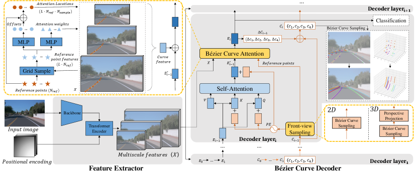
As shown in Figure 2, BézierFormer consists of a feature extractor and Bézier curve decoder. The feature extractor extracts multi-scale features of input images through a backbone network and a transformer encoder containing multi-scale deformable self-attention. The generated features are denoted as , where represents the number of feature map scales. The decoder consists of homogeneous layers indexed starting from 1. Decoder layeri receives features , Bézier control point queries and corresponding curve embeddings coming from Decoder layeri-1 as inputs. The Bézier control point queries model the shapes and positions of lane curves and are denoted as . is the number of queries, which means the maximum number of lane curves that BézierFormer can detect. Curve embeddings contain lane features and are denoted as . Decoder layeri outputs more precise control points and better embeddings for the next layer. For the first decoder layer, initial embeddings are randomly initialized learnable parameters. Initial control points could be initialized by . Because is related to the input image, this way brings a good generalization ability.
III-C Bézier Curve Decoder
Bézier curve decoder consists of layers with the same structure. It iteratively refines curve embeddings and control point queries. We employ a classification head for category recognition and use Bézier curve sampling defined by Eq.(1) to produce dense lane curve points for detection results.
Taking Decoder layeri as an example, the inputs are , , and . To leverage the geometric information of lane curves in self-attention and Bézier curve attention, the FV sampling module first sample points for each query. Then, using sine positional encoding and a MLP, we fuse the positions of these points and obtain the query’s positional encoding. The formula is:
| (3) |
After positional encoding, the relationships among lanes are modeled via multi-head self-attention, which enhances to better curve embeddings with global context:
| (4) |
and are single embeddings in and . is the index of the attention head. and are learnable parameters, where and are the feature dimensions of the embedding and the key in attention respectively. The attention weights are normalized to , and are learnable parameters.
Subsequent Bézier curve attention employs the points produced by FV sampling module as reference points. It collects curve features of each query from and updates to better embeddings for the next layer. A classification head calculates the category vectors from . A simple FFN predicts the offset , then the control points are refined as . To achieve layer-by-layer refinement, and of each layer need to be supervised.
III-D Bézier Curve Attention Mechanism
Bézier curve attention mechanism aims to better capture features of the slender lane curves represented by Bézier curves. We refrain from directly using vanilla deformable attention due to two primary reasons that render it suboptimal for extracting slender lane features. Firstly, deformable attention originates from object detection and generates only one reference point per object, but one reference point is insufficient to describe a slender lane curve comprehensively. Secondly, the reference points of deformable attention are adaptively generated, which causes slow convergence and less accurate lane feature extraction. To overcome these shortcomings, Bézier curve attention mechanism leverages Bézier curve sampling and Bézier curve attention operation to sample and fuse multiple reference points along the curve for accurate and comprehensive lane features.
The Bézier curve attention operation does not involve any interaction among , so we simplify the explanation of this operation by considering the update of a single . Let be the reference points. As shown in the left-top part of Figure 2, the features of the reference points at different scales of are sampled, then two MLPs calculate to obtain attention location offsets and attention weights for at scale . are added to to get the attention locations . To update , the formula is:
| (5) |
For simplicity, and represent and , respectively. , and have the same meanings as they have in Eq.(4). The dynamically generated attention weights are normalized to . Bézier curve attention operation extracts lane curve features from FV features and updates curve embeddings via Eq.(5). Enhanced curve embeddings are subsequently used for control points refinement and category recognition.
III-E Loss Function and Label Assignment
We present a lane regression loss derived from Chamfer Distance (CD) to better regress Bézier curve and use Focal Loss [20] for classification. [17] shows that regressing the sampled points can achieve better results than directly regressing Bézier control points. However, this method may sometimes be limited to optimizing the distance between local points, while ignoring the overall shape and location fit between two curves. We give an intuitive explanation of this limitation in the Appendix. We propose calculating CD between curves, as it considers each curve a whole entity to get the shortest distance from a point to the curve. As CD is calculated between point sets instead of continuous curves, points and on curve and are sampled. Inspired by [3], we give the lane curve a width and normalize CD to IoU, which we call Chamfer IoU, or CIoU for short. It is defined by:
| (6) |
The regression loss between a pair of predicted curve and ground truth curve can be formulated as:
| (7) |
However, the computation of CIoU ignores the order among the sampled points. To ensure the correct order of the sampled points, we add two simple geometric constraints.
| (8) |
| (9) |
means calculating the curve length. represent the normalized endpoints of the curve. Then, we get regression loss as and total loss is the sum of the losses of all decoder layers. The formula is:
| (10) |
To match predictions with ground truth, we adopt SimOTA [21] to dynamically assign predictions to each ground truth with the matching cost . Specifically, we set for an NMS-free pipeline.
IV Experiments
Datasets: We conduct experiments on two widely-used 2D and 3D lane detection benchmarks. CurveLanes [1] is a large-scale 2D lane dataset with complex lane topologies. It comprises 150,000 images for training, validation, and testing. In CurveLanes, curved lanes account for over 90%, encompassing challenging cases such as dense, forked, merged, and nearly horizontal lanes. OpenLane [6] is a recently released large-scale real-world 3D lane dataset, with a total of 200,000 images and over 880,000 3D annotations.
Evaluation Metric: To keep consistent with [1], we use F1 score for 2D lane detection evaluation. For OpenLane, we follow [6] to report the F1 score and category accuracy.
Implementation Details: We choose ResNet18 [22] and Swin-Tiny [23] as pre-trained backbones. Input images are resized to on CurveLanes, and on OpenLane. We set for CurveLanes and OpenLane to 16 and 32, respectively. We train 24 epochs with batch size 16, using an AdamW optimizer with a learning rate of 1e-4. We set to 0, 0.25, 0.5, 0.75, and 1 to obtain reference points, and . To calculate , we set and lane width for CurveLanes, for OpenLane. More details are in the Appendix.
IV-A Comparisons with the State-of-the-Art Methods
IV-A1 2D lane detection
Table I shows BézierFormer achieves top-tier performance on CurveLanes. Even based on ResNet18, BézierFormer achieves a better F1 score of 89.06% than CLRNet’s 86.48% based on ResNet101. With Swin-Tiny as the backbone, BézierFormer achieves a state-of-the-art F1 score of 91.06%, which is 4.58% higher than that of CLRNet. Compared to the best bottom-up method RCLane, BézierFormer achieves a comparable performance but a much higher inference efficiency. The results on CurveLanes indicate that BézierFormer is effective and effecient in 2D lane detection. We give more qualitative visualized results in the Appendix.
| Method | Backbone | F1 (%) | P (%) | R (%) | FPS |
| SCNN[12]† | VGG16 | 65.02 | 76.13 | 56.74 | 8 |
| PointLaneNet[15]† | ResNet101 | 78.47 | 86.33 | 72.91 | - |
| CurveLane-L[1]† | - | 82.29 | 81.11 | 75.03 | - |
| CondLaneNet[2]‡ | ResNet101 | 86.1 | 88.98 | 83.41 | 48 |
| UFLDv2[5]‡ | ResNet34 | 81.34 | 81.93 | 80.76 | 86 |
| CLRNet[3]§ | ResNet101 | 86.48 | 91.77 | 81.76 | 74 |
| RCLane[4]‡ | SegFormer | 91.43 | 93.96 | 89.03 | 25 |
| BézierFormer | ResNet18 | 89.06 | 93.57 | 84.96 | 133 |
| BézierFormer | Swin-Tiny | 91.31 | 93.81 | 88.94 | 84 |
IV-A2 3D lane detection
Table II shows that BézierFormer achieves state-of-the-art performance on OpenLane. With the input resolution of , BézierFormer achieves an F1 score of 56.43% and a category accuracy of 94.1%, which are 2.73% and 3.2% higher than those of the second-best Anchor3DLane, and has a higher FPS. It is worth noting that NMS-free BézierFormer only uses 32 queries, while Anchor3Dlane needs over 4,000 3D lane anchors. CurveFormer is also a DETR-like method but represents lane curves as 3D point sets. BézierFormer outperforms CurveFormer by 5.93% F1 score and is superior in all scenarios and X/Z errors, indicating that Bézier curve is a better representation of 3D lane curves than 3D point sets. With a larger input resolution of , BézierFormer achieves a higher F1 score of 58.6% and a category accuracy of 94.2%. Tabele II demonstrates BézierFormer’s effectiveness and efficiency in 3D lane detection. More qualitative results of BézierFormer are in the Appendix.
| Method | Backbone | F1(%) | Cate Acc(%) | FPS |
| 3D-LaneNet[18]† | VGG16 | 44.1 | - | - |
| Gen-LaneNet[19]† | ERFNet | 32.3 | - | - |
| PersFormer[6]‡ | EfficientNet | 50.5 | 92.3 | 15 |
| CurveFormer[8]‡ | EfficientNet | 50.5 | - | - |
| Anchor3DLane[7]‡ | ResNet18 | 53.7 | 90.9 | 74 |
| BézierFormer | ResNet18 | 53.84 | 92.02 | 151 |
| BézierFormer | Swin-Tiny | 56.43 | 94.1 | 90 |
| BézierFormer | Swin-Tiny | 58.6 | 94.2 | 42 |
IV-B Ablation Studies
In this section, we conduct all the studies with ResNet18.
IV-B1 Lane Representation
To demonstrate the superiority of Bézier curve in lane detection, we compare it with polynomial and row-based representations. The polynomial and row-based representations are referenced to LSTR[24] and CurveFormer[8], respectively. For fairness, we adapt these representations into an architecture akin to BézierFormer, detailed in the Appendix, and use advanced LineIoU loss [3] for better performance. Table III reveals that Bézier curve yields much better results.
| Method | Poly | Row-based | Bézier Curve |
| (%) | 80.90 | 83.10 | 89.06 |
| (%) | 50.30 | 51.27 | 53.84 |
IV-B2 Attention mechanism
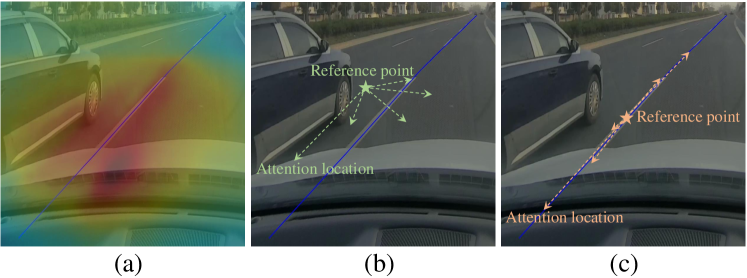
To validate the superiority of our Bézier curve attention mechanism in lane detection, we compare it with ordinary attention [25] and vanilla deformable attention. Vanilla deformable attention only adaptively generates one reference point, so Bézier curve attention uses to sample one reference point for fairness. As shown in Table IV, Bézier curve attention mechanism obviously brings better performance through explicitly sampling reference points. Figure 3 also illustrates that Bézier curve attention has more precise attention locations than the other two attention mechanisms.
| Method | Ordinary | Deformable | Bézier Curve |
| (%) | 82.76 | 85.81 | 87.60 |
| (%) | 46.53 | 49.08 | 52.13 |
IV-B3 Loss Function
On CurveLanes, we compare our Chamfer IoU-based regression loss with the sampling loss [17] for Bézier curve fitting. For fairness, we normalize the sampling distance between curves’ points to IoU and get sampling IoU loss. Table V indicates that our regression loss performs better because Chamfer IoU measures overall shape and location similarity between curves better.
| Method | Sampling | Sampling IoU | Ours |
| (%) | 78.78 | 81.86 | 89.06 |
| (%) | 47.11 | 48.32 | 53.84 |
V Conclusion
In this work, we introduce BézierFormer, a novel unified 2D/3D lane detection architecture. It employs Bézier control point queries to represent lane curves and uses a novel Bézier curve attention mechanism to accurately and comprehensively extract lane features. Besides, we propose the Chamfer IoU-based regression loss to improve the performance. Finally, its state-of-the-art performance on widely-used 2D and 3D lane detection benchmarks attests to BézierFormer’s effectiveness in both 2D and 3D lane detection and suggests that further exploration would be valuable.
VI Appendix
VI-A Implementation Details
We implement BézierFormer based on MMDetection [26]. For reproducibility, we give the detailed experimental settings, including hyperparameters of the training and testing process, data augmentation strategies, and network settings of BézierFormer in Table VI.
| Dataset | CULane | CurveLanes | OpenLane |
| Input resolution | |||
| Epochs | 24 | 24 | 24 |
| Batch size | 16 | 16 | 16 |
| Optimizer | AdamW | AdamW | AdamW |
| LR | 0.0001 | 0.0001 | 0.0001 |
| LR of backbone | 0.00001 | 0.00001 | 0.00001 |
| LR decay | Poly | Poly | Poly |
| LR decay setting | power=2,min=1e-5 | power=2,min=1e-5 | power=2,min=1e-5 |
| Weight decay | 0.0001 | 0.0001 | 0.0001 |
| Warmup epochs | None | None | None |
| Horizontal flip | yes | yes | no |
| RandomAffine | yes | yes | no |
| Color jitter | yes | yes | no |
| Blur | yes | yes | no |
| RandomBrightness | yes | yes | no |
| Control points dimension | 2 | 2 | 3 |
| Perspective projection | no | no | yes |
| Nquery | 10 | 16 | 32 |
| Nref | 5 | 5 | 5 |
| Nsample | 5 | 5 | 5 |
| Ndis | 200 | 200 | 200 |
| e(width of lane curve) | 10 | 10 | 0.9 |
| Dimension of Ei | Res18:128,Swin-T:256 | Res18:128,Swin-T:256 | Res18:256,Swin-T:256 |
| Number of feature scales | 4 | 4 | 4 |
| Number of decoder layers | 6 | 6 | 6 |
VI-B Illustration of Loss Function
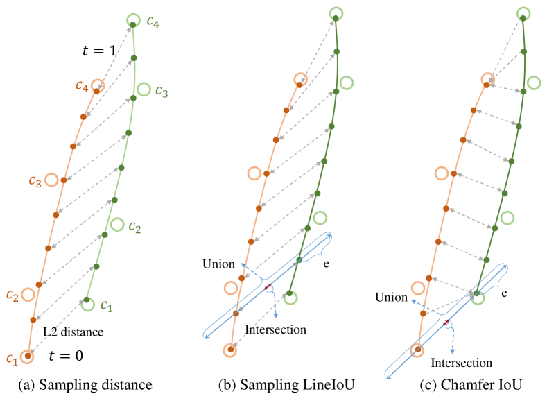
For a more intuitive understanding of the advantage of Chamfer IoU-based lane regression loss, Figure 4 visualizes different losses. Figure 4(c) shows that the distances between two curves’ endpoints are relatively larger than other locations, contributing to a more effective learning process compared with Figure 4(a) and Figure 4(b).
VI-C Poly and Row-based Curve Decoder
For a fair comparison with polynomial and row-based lane representation, we employ the same feature extractor and design delicated decoders for them, similar with Bézier curve decoder as shown in Figure 5.
For polynomial representation, we refer to LSTR [16] and use to formulate a curve. LSTR uses vertical as variable to describe a curve, is the polynomial parameters, represents the coordinates of endpoints. The formula is:
| (11) |
To sample the reference points for Poly Curve Attention, which has the same equation with Bézier Curve Attention, we selects five equally-spaced coordinates:
| (12) |
Thus, we can get the reference points of Poly Curve Attention according to Eq.(11). Finally, the reference points are:
| (13) |
For row-based representation, we refer to Laneformer [27]. Laneformer formulates a lane curve as , where are the coordinates for the 72 equally-spaced coordinates, and denote for the start coordinate and end coordinate of the curve. Row-based Curve Attention also shares the same equation with Bézier Curve Attention, but has a different reference points sampling method. To get the five reference points, we compute five equally-spaced indexes of according to and , as follows.
| (14) |
Then we can get the five reference points:
| (15) |
VI-D Results on CULane
CULane [12] is also a famous large-scale 2D lane detection dataset including nine challenging scenarios on highways and urban roads. CULane’s challenge lies in various difficult visual scenes. Although BézierFormer is not designed with this challenge in mind, it still slightly outperforms methods which are proposed to address this challenge, such as CLRNet [3], on CULane.
| Method | Backbone | mF1(%) | F1(%) | F1@75(%) | Normal | Crowd | Hlight | Shadow | NoLine | Arrow | Curve | Cross | Night |
| Bottom-Up: | |||||||||||||
| RESA[13]† | ResNet50 | 47.86 | 75.3 | 53.39 | 92.1 | 73.1 | 69.2 | 72.8 | 47.7 | 88.3 | 70.3 | 1503 | 69.9 |
| FOLOLane[14]‡ | ERFNet | - | 78.8 | - | 92.7 | 77.8 | 75.2 | 79.3 | 52.1 | 89 | 69.4 | 1569 | 74.5 |
| GANet[28]§ | ResNet101 | 54.71 | 79.63 | 62.33 | 93.67 | 78.66 | 71.82 | 78.32 | 53.38 | 89.86 | 77.37 | 1352 | 73.85 |
| RCLane[4]‡ | SegFormer | - | 80.5 | - | 94.01 | 79.13 | 72.92 | 81.16 | 53.94 | 90.51 | 79.66 | 931 | 75.1 |
| Top-Down: | |||||||||||||
| UFLDv2[5]§ | ResNet34 | 49.94 | 76 | 55.49 | 92.5 | 74.8 | 65.5 | 75.5 | 49.2 | 88.8 | 70.1 | 1910 | 70.8 |
| LaneATT[29]† | ResNet122 | 51.48 | 77.02 | 57.5 | 91.74 | 76.16 | 69.47 | 76.31 | 50.46 | 86.29 | 64.05 | 1264 | 70.81 |
| LSTR[24]§ | ResNet18 | 35.93 | 68.72 | 34.23 | 86.78 | 67.34 | 56.63 | 59.82 | 40.1 | 78.66 | 56.64 | 1166 | 59.92 |
| CondLaneNet[2]† | ResNet101 | 54.83 | 79.48 | 61.23 | 93.47 | 77.44 | 70.93 | 90.91 | 54.13 | 90.16 | 75.21 | 1201 | 74.8 |
| LaneFormer[27]‡ | ResNet50 | - | 77.06 | - | 91.77 | 75.41 | 70.17 | 75.75 | 48.73 | 87.65 | 66.33 | 19 | 71.04 |
| BézierLaneNet§ | ResNet34 | 49.24 | 75.57 | 53.91 | 91.59 | 73.2 | 69.2 | 76.74 | 48.05 | 87.16 | 62.45 | 888 | 69.9 |
| CLRNet[3]† | ResNet18 | 55.23 | 79.58 | 62.1 | 93.3 | 78.33 | 73.71 | 79.66 | 53.14 | 90.25 | 71.56 | 1321 | 75.11 |
| CLRNet[3]† | ResNet101 | 55.55 | 80.13 | 62.96 | 93.85 | 78.78 | 72.49 | 82.33 | 54.5 | 89.79 | 75.57 | 1262 | 75.51 |
| CLRNet[3]† | DLA34 | 55.64 | 80.47 | 62.78 | 93.73 | 79.59 | 75.3 | 82.51 | 54.58 | 90.62 | 74.13 | 1155 | 75.37 |
| BézierFormer | ResNet18 | 55.32 | 79.44 | 62.61 | 93.07 | 77.52 | 74.45 | 75.48 | 52.57 | 89.91 | 71.89 | 1580 | 74.39 |
| BézierFormer | Swin-Tiny | 57.07 | 80.63 | 63.95 | 93.71 | 78.7 | 74.93 | 81.73 | 55.09 | 90.06 | 73.61 | 1025 | 76.93 |
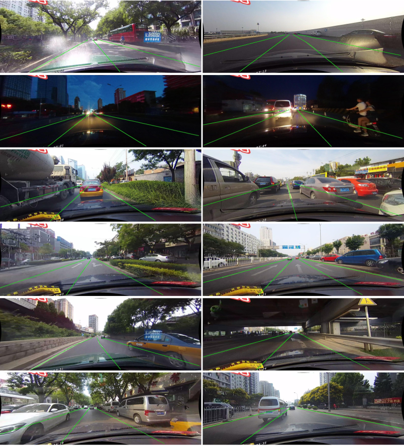
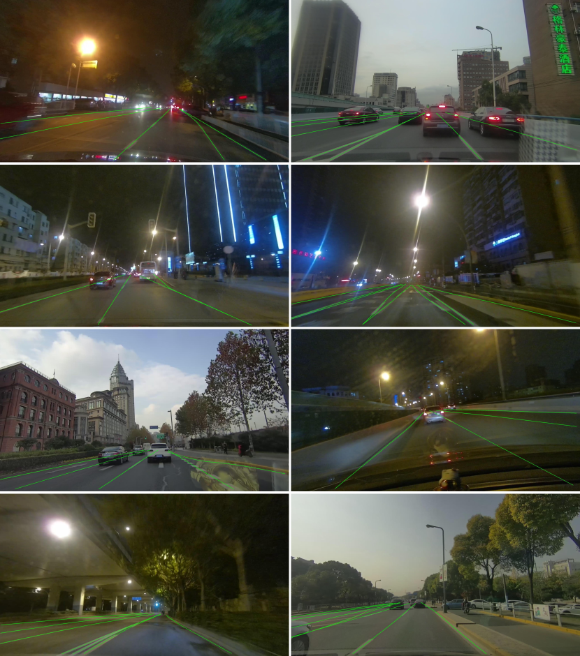
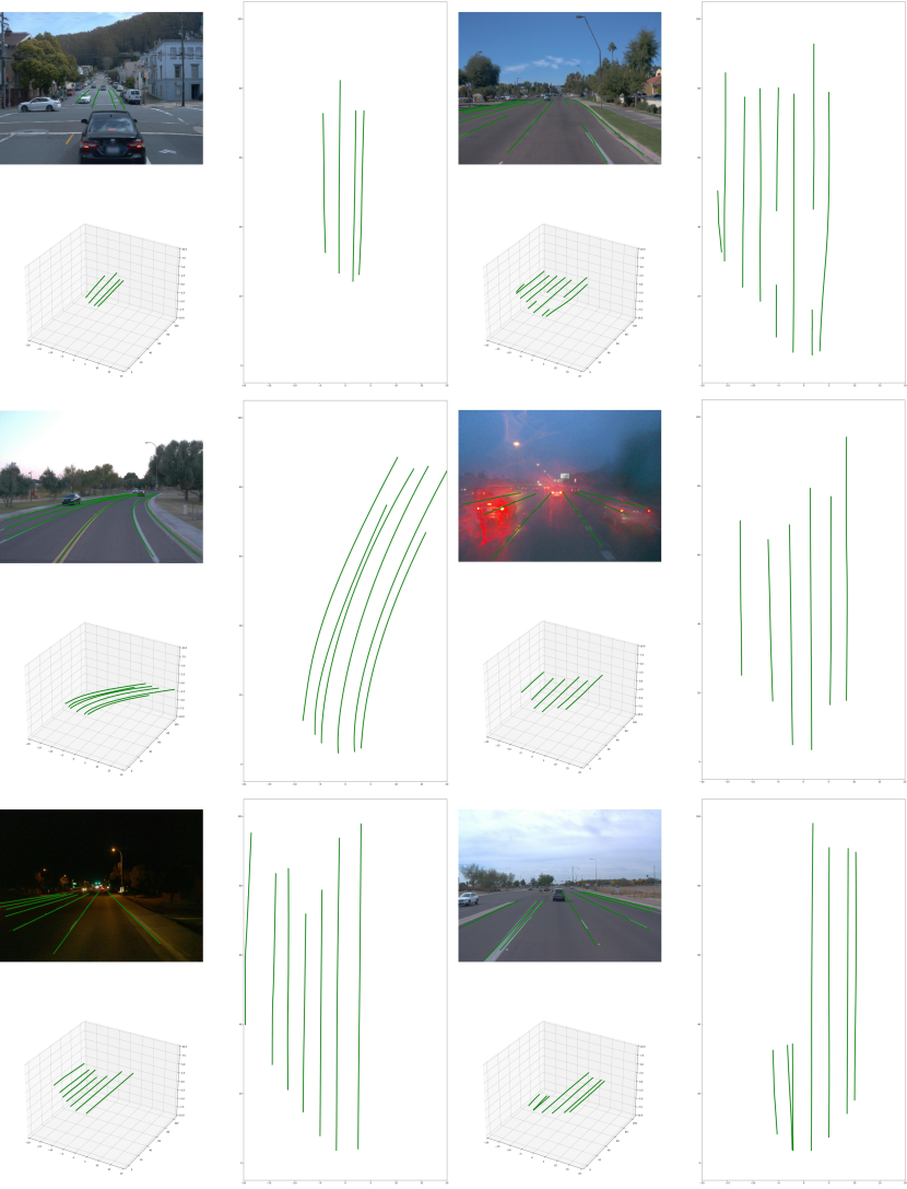
VI-E Qualitative Results
To have an intuitive understanding of the performance of BézierFormer, we give the qualitative results on CULane [12], CurveLanes [1] and OpenLane [6]. As shown in Figure 6, BézierFormer is robust in challenging scenarios like Highlight, Night, Crowd, Arrow, Curve, Shadow, and No Line. Figure 7 shows the results on CurveLanes and indicates that BézierFormer performs well in complex topologies like merged lanes, forked lanes, curves lanes, dense lanes, and nearly horizontal lanes. Figure 8 draws the results on OpenLane and proves the effectiveness of BézierFormer’s 3D lane detection in different scenes.
References
- [1] Hang Xu, Shaoju Wang, Xinyue Cai, Wei Zhang, Xiaodan Liang, and Zhenguo Li, “Curvelane-nas: Unifying lane-sensitive architecture search and adaptive point blending,” in Computer Vision–ECCV 2020: 16th European Conference, Glasgow, UK, August 23–28, 2020, Proceedings, Part XV 16. Springer, 2020, pp. 689–704.
- [2] Lizhe Liu, Xiaohao Chen, Siyu Zhu, and Ping Tan, “Condlanenet: a top-to-down lane detection framework based on conditional convolution,” in Proceedings of the IEEE/CVF International Conference on Computer Vision, 2021, pp. 3773–3782.
- [3] Tu Zheng, Yifei Huang, Yang Liu, Wenjian Tang, Zheng Yang, Deng Cai, and Xiaofei He, “Clrnet: Cross layer refinement network for lane detection,” in Proceedings of the IEEE/CVF conference on computer vision and pattern recognition, 2022, pp. 898–907.
- [4] Shenghua Xu, Xinyue Cai, Bin Zhao, Li Zhang, Hang Xu, Yanwei Fu, and Xiangyang Xue, “Rclane: Relay chain prediction for lane detection,” in ECCV, 2022.
- [5] Zequn Qin, Pengyi Zhang, and Xi Li, “Ultra fast deep lane detection with hybrid anchor driven ordinal classification,” IEEE transactions on pattern analysis and machine intelligence, 2022.
- [6] Li Chen, Chonghao Sima, Yang Li, Zehan Zheng, Jiajie Xu, Xiangwei Geng, Hongyang Li, Conghui He, Jianping Shi, Yu Qiao, et al., “Persformer: 3d lane detection via perspective transformer and the openlane benchmark,” in European Conference on Computer Vision. Springer, 2022, pp. 550–567.
- [7] Shaofei Huang, Zhenwei Shen, Zehao Huang, Zi-han Ding, Jiao Dai, Jizhong Han, Naiyan Wang, and Si Liu, “Anchor3dlane: Learning to regress 3d anchors for monocular 3d lane detection,” in Proceedings of the IEEE/CVF Conference on Computer Vision and Pattern Recognition, 2023, pp. 17451–17460.
- [8] Yifeng Bai, Zhirong Chen, Zhangjie Fu, Lang Peng, Pengpeng Liang, and Erkang Cheng, “Curveformer: 3d lane detection by curve propagation with curve queries and attention,” in 2023 IEEE International Conference on Robotics and Automation (ICRA). IEEE, 2023, pp. 7062–7068.
- [9] Nicolas Carion, Francisco Massa, Gabriel Synnaeve, Nicolas Usunier, Alexander Kirillov, and Sergey Zagoruyko, “End-to-end object detection with transformers,” in European conference on computer vision. Springer, 2020, pp. 213–229.
- [10] Shilong Liu, Feng Li, Hao Zhang, Xiao Yang, Xianbiao Qi, Hang Su, Jun Zhu, and Lei Zhang, “DAB-DETR: Dynamic anchor boxes are better queries for DETR,” in International Conference on Learning Representations, 2022.
- [11] Xizhou Zhu, Weijie Su, Lewei Lu, Bin Li, Xiaogang Wang, and Jifeng Dai, “Deformable detr: Deformable transformers for end-to-end object detection,” arXiv preprint arXiv:2010.04159, 2020.
- [12] Xingang Pan, Jianping Shi, Ping Luo, Xiaogang Wang, and Xiaoou Tang, “Spatial as deep: Spatial cnn for traffic scene understanding,” in Proceedings of the AAAI Conference on Artificial Intelligence, 2018, vol. 32.
- [13] Tu Zheng, Hao Fang, Yi Zhang, Wenjian Tang, Zheng Yang, Haifeng Liu, and Deng Cai, “Resa: Recurrent feature-shift aggregator for lane detection,” in Proceedings of the AAAI Conference on Artificial Intelligence, 2021, vol. 35, pp. 3547–3554.
- [14] Zhan Qu, Huan Jin, Yang Zhou, Zhen Yang, and Wei Zhang, “Focus on local: Detecting lane marker from bottom up via key point,” in Proceedings of the IEEE/CVF Conference on Computer Vision and Pattern Recognition, 2021, pp. 14122–14130.
- [15] Zhenpeng Chen, Qianfei Liu, and Chenfan Lian, “Pointlanenet: Efficient end-to-end cnns for accurate real-time lane detection,” in 2019 IEEE intelligent vehicles symposium (IV). IEEE, 2019, pp. 2563–2568.
- [16] Ruijin Liu, Zejian Yuan, Tie Liu, and Zhiliang Xiong, “End-to-end lane shape prediction with transformers,” in Proceedings of the IEEE/CVF winter conference on applications of computer vision, 2021, pp. 3694–3702.
- [17] Zhengyang Feng, Shaohua Guo, Xin Tan, Ke Xu, Min Wang, and Lizhuang Ma, “Rethinking efficient lane detection via curve modeling,” in Proceedings of the IEEE/CVF Conference on Computer Vision and Pattern Recognition, 2022, pp. 17062–17070.
- [18] Noa Garnett, Rafi Cohen, Tomer Pe’er, Roee Lahav, and Dan Levi, “3d-lanenet: end-to-end 3d multiple lane detection,” in Proceedings of the IEEE/CVF International Conference on Computer Vision, 2019, pp. 2921–2930.
- [19] Yuliang Guo, Guang Chen, Peitao Zhao, Weide Zhang, Jinghao Miao, Jingao Wang, and Tae Eun Choe, “Gen-lanenet: A generalized and scalable approach for 3d lane detection,” in Computer Vision–ECCV 2020: 16th European Conference, Glasgow, UK, August 23–28, 2020, Proceedings, Part XXI 16. Springer, 2020, pp. 666–681.
- [20] Tsung-Yi Lin, Priya Goyal, Ross Girshick, Kaiming He, and Piotr Dollár, “Focal loss for dense object detection,” in Proceedings of the IEEE international conference on computer vision, 2017, pp. 2980–2988.
- [21] Zheng Ge, Songtao Liu, Feng Wang, Zeming Li, and Jian Sun, “Yolox: Exceeding yolo series in 2021,” arXiv preprint arXiv:2107.08430, 2021.
- [22] Kaiming He, Xiangyu Zhang, Shaoqing Ren, and Jian Sun, “Deep residual learning for image recognition,” in Proceedings of the IEEE Conference on Computer Vision and Pattern Recognition (CVPR), June 2016.
- [23] Ze Liu, Yutong Lin, Yue Cao, Han Hu, Yixuan Wei, Zheng Zhang, Stephen Lin, and Baining Guo, “Swin transformer: Hierarchical vision transformer using shifted windows,” in Proceedings of the IEEE/CVF International Conference on Computer Vision (ICCV), October 2021, pp. 10012–10022.
- [24] Ruijin Liu, Dapeng Chen, Tie Liu, Zhiliang Xiong, and Zejian Yuan, “Learning to predict 3d lane shape and camera pose from a single image via geometry constraints,” in Proceedings of the AAAI Conference on Artificial Intelligence, 2022, vol. 36, pp. 1765–1772.
- [25] Ashish Vaswani, Noam Shazeer, Niki Parmar, Jakob Uszkoreit, Llion Jones, Aidan N Gomez, Łukasz Kaiser, and Illia Polosukhin, “Attention is all you need,” Advances in neural information processing systems, vol. 30, 2017.
- [26] Kai Chen, Jiaqi Wang, Jiangmiao Pang, Yuhang Cao, Yu Xiong, Xiaoxiao Li, Shuyang Sun, Wansen Feng, Ziwei Liu, Jiarui Xu, Zheng Zhang, Dazhi Cheng, Chenchen Zhu, Tianheng Cheng, Qijie Zhao, Buyu Li, Xin Lu, Rui Zhu, Yue Wu, Jifeng Dai, Jingdong Wang, Jianping Shi, Wanli Ouyang, Chen Change Loy, and Dahua Lin, “MMDetection: Open mmlab detection toolbox and benchmark,” arXiv preprint arXiv:1906.07155, 2019.
- [27] Jianhua Han, Xiajun Deng, Xinyue Cai, Zhen Yang, Hang Xu, Chunjing Xu, and Xiaodan Liang, “Laneformer: Object-aware row-column transformers for lane detection,” in Proceedings of the AAAI Conference on Artificial Intelligence, 2022, vol. 36, pp. 799–807.
- [28] Jinsheng Wang, Yinchao Ma, Shaofei Huang, Tianrui Hui, Fei Wang, Chen Qian, and Tianzhu Zhang, “A keypoint-based global association network for lane detection,” in Proceedings of the IEEE/CVF Conference on Computer Vision and Pattern Recognition, 2022, pp. 1392–1401.
- [29] Lucas Tabelini, Rodrigo Berriel, Thiago M Paixao, Claudine Badue, Alberto F De Souza, and Thiago Oliveira-Santos, “Keep your eyes on the lane: Real-time attention-guided lane detection,” in Proceedings of the IEEE/CVF conference on computer vision and pattern recognition, 2021, pp. 294–302.