Northeastern University
Boston, MA 02115, USA
11email: {wang.dian, kohler.c, zhu.xup, jia.ming, r.platt}@northeastern.edu 000*Equal Contribution
BulletArm: An Open-Source Robotic Manipulation Benchmark and Learning Framework
Abstract
We present BulletArm, a novel benchmark and learning-environment for robotic manipulation. BulletArm is designed around two key principles: reproducibility and extensibility. We aim to encourage more direct comparisons between robotic learning methods by providing a set of standardized benchmark tasks in simulation alongside a collection of baseline algorithms. The framework consists of 31 different manipulation tasks of varying difficulty, ranging from simple reaching and picking tasks to more realistic tasks such as bin packing and pallet stacking. In addition to the provided tasks, BulletArm has been built to facilitate easy expansion and provides a suite of tools to assist users when adding new tasks to the framework. Moreover, we introduce a set of five benchmarks and evaluate them using a series of state-of-the-art baseline algorithms. By including these algorithms as part of our framework, we hope to encourage users to benchmark their work on any new tasks against these baselines.
keywords:
Benchmark, Simulation, Robotic Learning, Reinforcement Learning1 Introduction
Inspired by the recent successes of deep learning in the field of computer vision, there has been an explosion of work aimed at applying deep learning algorithms across a variety of disciplines. Deep reinforcement learning, for example, has been used to learn policies which achieve superhuman levels of performance across a variety of games [36, 30]. Robotics has seen a similar surge in recent years, especially in the area of robotic manipulation with reinforcement learning [12, 20, 51], imitation learning [50], and multi-task learning [10, 14]. However, there is a key difference between current robotics learning research and past work applying deep learning to other fields. There currently is no widely accepted standard for comparing learning-based robotic manipulation methods. In computer vision for example, the ImageNet benchmark [8] has been a crucial factor in the explosion of image classification algorithms we have seen in the recent past.
While there are benchmarks for policy learning in domains similar to robotic manipulation, such as the continuous control tasks in OpenAI Gym [4] and the DeepMind Control Suite [37], they are not applicable to more real-world tasks we are interested in robotics. Furthermore, different robotics labs work with drastically different systems in the real-world using different robots, sensors, etc. As a result, researchers often develop their own training and evaluation environments, making it extremely difficult to compare different approaches. For example, even simple tasks like block stacking can have a lot of variability between different works [31, 28, 43], including different physics simulators, different manipulators, different object sizes, etc.
In this work, we introduce BulletArm, a novel framework for robotic manipulation learning based on two key components. First, we provide a flexible, open-source framework that supports many different manipulation tasks. Compared with prior works, we introduce tasks with various difficulties and require different manipulation skills. This includes long-term planning tasks like supervising Covid tests and contact-rich tasks requiring precise nudging or pushing behaviors. BulletArm currently consists of 31 unique tasks which the user can easily customize to mimic their real-world lab setups (e.g., workspace size, robotic arm type, etc). In addition, BulletArm was developed with a emphasis on extensability so new tasks can easily be created as needed. Second, we include five different benchmarks alongside a collection of standardized baselines for the user to quickly benchmark their work against. We include our implementations of these baselines in the hopes of new users applying them to their customization of existing tasks and whatever new tasks they create.
Our contribution can be summarized as three-fold. First, we propose BulletArm, a benchmark and learning framework containing a set of 21 open-loop manipulation tasks and 10 close-loop manipulation tasks. We have developed this framework over the course of many prior works [43, 3, 45, 3, 44, 42, 54]. Second, we provide state-of-the-art baseline algorithms enabling other researchers to easily compare their work against our baselines once new tasks are inevitably added to the baseline. Third, BulletArm provides a extensive suite of tools to allow users to easily create new tasks as needed. Our code is available at https://github.com/ColinKohler/BulletArm.
2 Related Work
Reinforcement Learning Environments
Standardized environments are vitally important when comparing different reinforcement learning algorithms. Many prior works have developed various video game environments, including PacMan [33], Super Mario [39], Doom [21], and StarCraft [41]. OpenAI Gym [4] provides a standard API for the communication between agents and environments, and a collection of various different environments including Atari games from the Arcade Learning Environment (ALE) [2] and some robotic tasks implemented using MuJoCo [38]. The DeepMind Control Suite (DMC) [37] provides a similar set of continuous control tasks. Although both OpenAI Gym and DMC have a small set of robotic environments, they are toy tasks which are not representative of the real-world tasks we are interested in robotics.
Robotic Manipulation Environments
In robotic manipulation, there are many benchmarks for grasping in the context of supervised learning, e.g., the Cornell dataset [19], the Jacquard dataset [9], and the GraspNet 1B dataset [11]. In the context of reinforcement learning, on the other hand, the majority of prior frameworks focus on single tasks, for example, door opening [40], furniture assembly [27], and in-hand dexterous manipulation [1]. Another strand of prior works propose frameworks containing a variety of different environments, such as robosuite [55], PyRoboLearn [7], and Meta-World [48], but are often limited to short horizon tasks. Ravens [50] introduces a set of environments containing complex manipulation tasks but restricts the end-effector to a suction cup gripper. RLBench [18] provides a similar learning framework to ours with a number of key differences. First, RLBench is built around the PyRep [17] interface and is therefor built on-top of V-REP [34]. Furthermore, RLBench is more restrictive than BulletArm with limitations placed on the workspace scene, robot, and more.
Robotic Manipulation Control
There are two commonly used end-effector control schemes: open-loop control and close-loop control. In open-loop control, the agent selects both the target pose of target pose of the end-effector and some action primitive to execute at that pose. Open-loop control generally has shorter time horizon, allowing the agent to solve complex tasks that require a long trajectory [52, 51, 43]. In close-loop control, the agent sets the displacement of the end-effector This allows the agent to more easily recover from failures which is vital when delaing with contact-rich tasks [12, 20, 53, 44]. BulletArm provides a collection of environments in both settings, allowing the users to select either one based on their research interests.
3 Architecture
At the core of our learning framework is the PyBullet [6] simulator. PyBullet is a Python library for robotics simulation and machine learning with a focus on sim-to-real transfer. Built upon Bullet Physics SDK, PyBullet provides access to forward dynamics simulation, inverse dynamics computation, forward and inverse kinematics, collision detection, and more. In addition to physics simulation, there are also numerous tools for scene rendering and visualization. BulletArm builds upon PyBullet, providing a diverse set of tools tailored to robotic manipulation simulations.
3.1 Design Philosophy
The design philosophy behind our framework focuses on four key principles:
1. Reproducibility: A key challenge when developing new learning algorithms is the difficulty in comparing them to previous work. In robotics, this problem is especially prevalent as different researchers have drastically different robotic setups. This can range from small differences, such as workspace size or degradation of objects, to large differences such as the robot used to preform the experiments. Moving to simulation allows for the standardization of these factors but can impact the performance of the trained algorithm in the real-world. We aim to encourage more direct comparisons between works by providing a flexible simulation environment and a number of baselines to compare against.
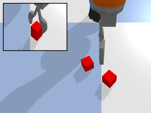
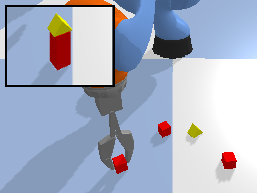
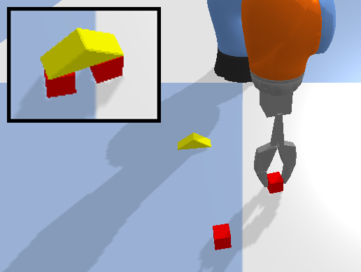
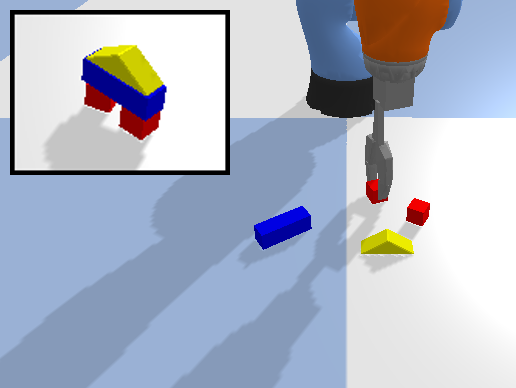
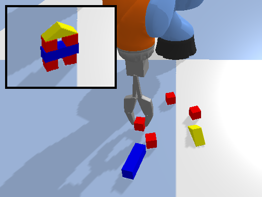
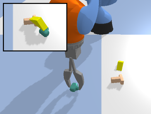
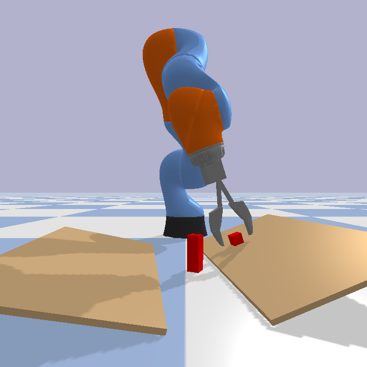
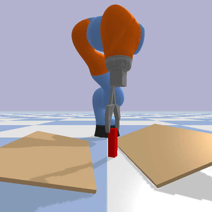
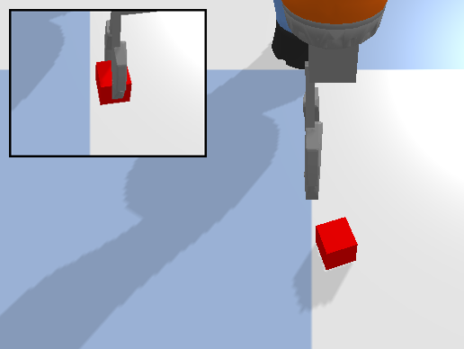
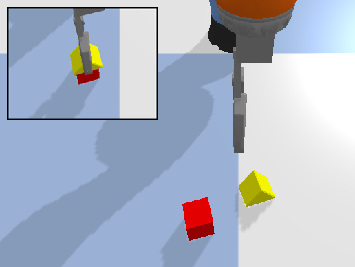
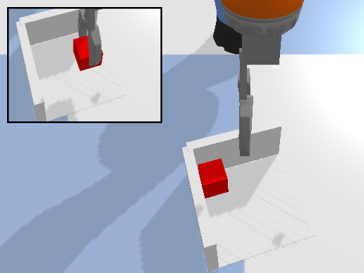
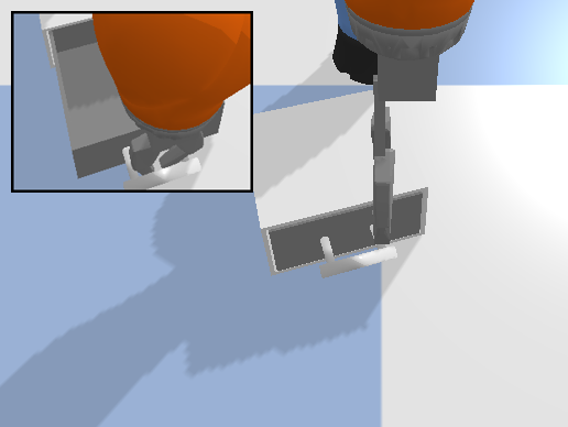
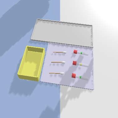
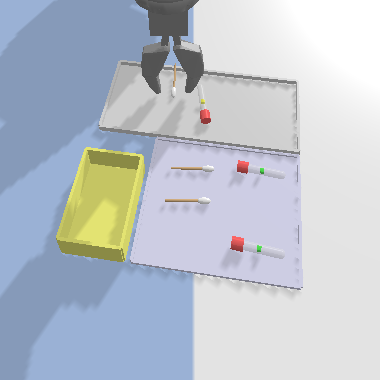
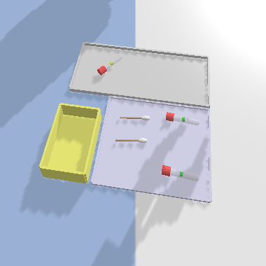
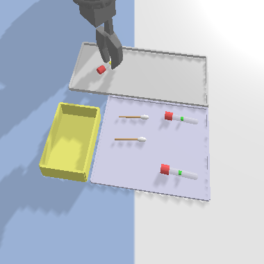
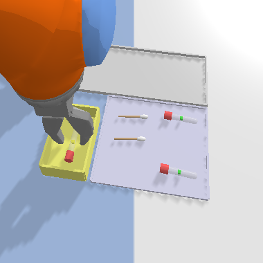
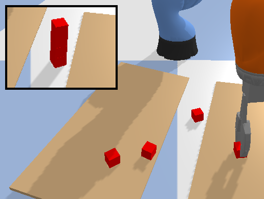
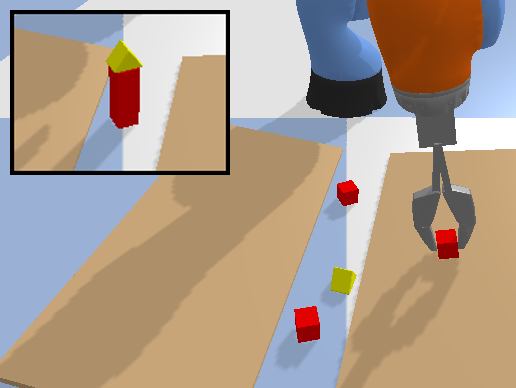
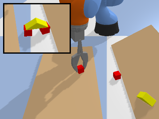
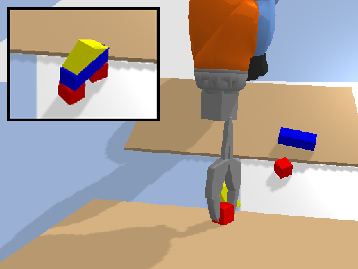
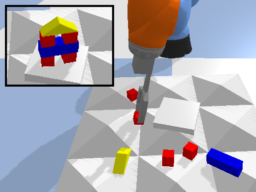
2. Extensibility: Although we include a number of tasks, control types, and robots; there will always be a need for additional development in these areas. Using our framework, users can easily add new tasks, robots, and objects. We make the choice to not restrict tasks, allowing users more freedom create interesting domains. Figure 1 shows an example of creating a new task using our framework.
3. Performance: Deep learning methods are often time consuming, slow processes and the addition of a physics simulator can lead to long training times. We have spent a significant portion of time in ensuring that our framework will not bottleneck training by optimizing the simulations and allowing the user to run many environments in parallel.
4. Usability: A good open-source framework should be easy to use and understand. We provide extensive documentation detailing the key components of our framework and a set of tutorials demonstrating both how to use the environments and how to extend them.
3.2 Environment
|
1from bulletarm.base_env import BaseEnv
2from bulletarm.constants import CUBE
3
4class PyramidStackEnv(BaseEnv):
5 def __init__(self, config):
6 super().__init__(config)
7
8 def reset(self):
9 self.resetPybulletWorkspace()
10 self.cubes = self._generateShapes(CUBE, 3)
11 return self._getObservation()
12
13 def _checkTermination(self):
14 return self.areBlocksInPyramid(self.cubes)
|
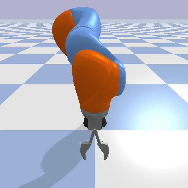
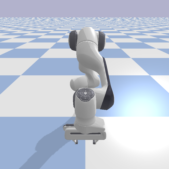
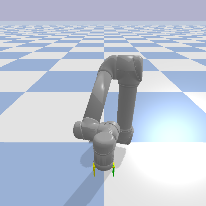
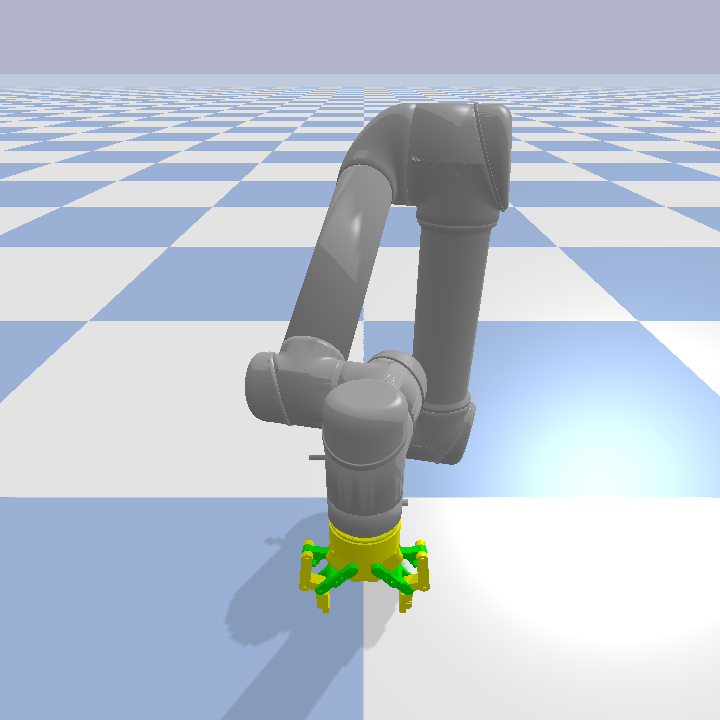
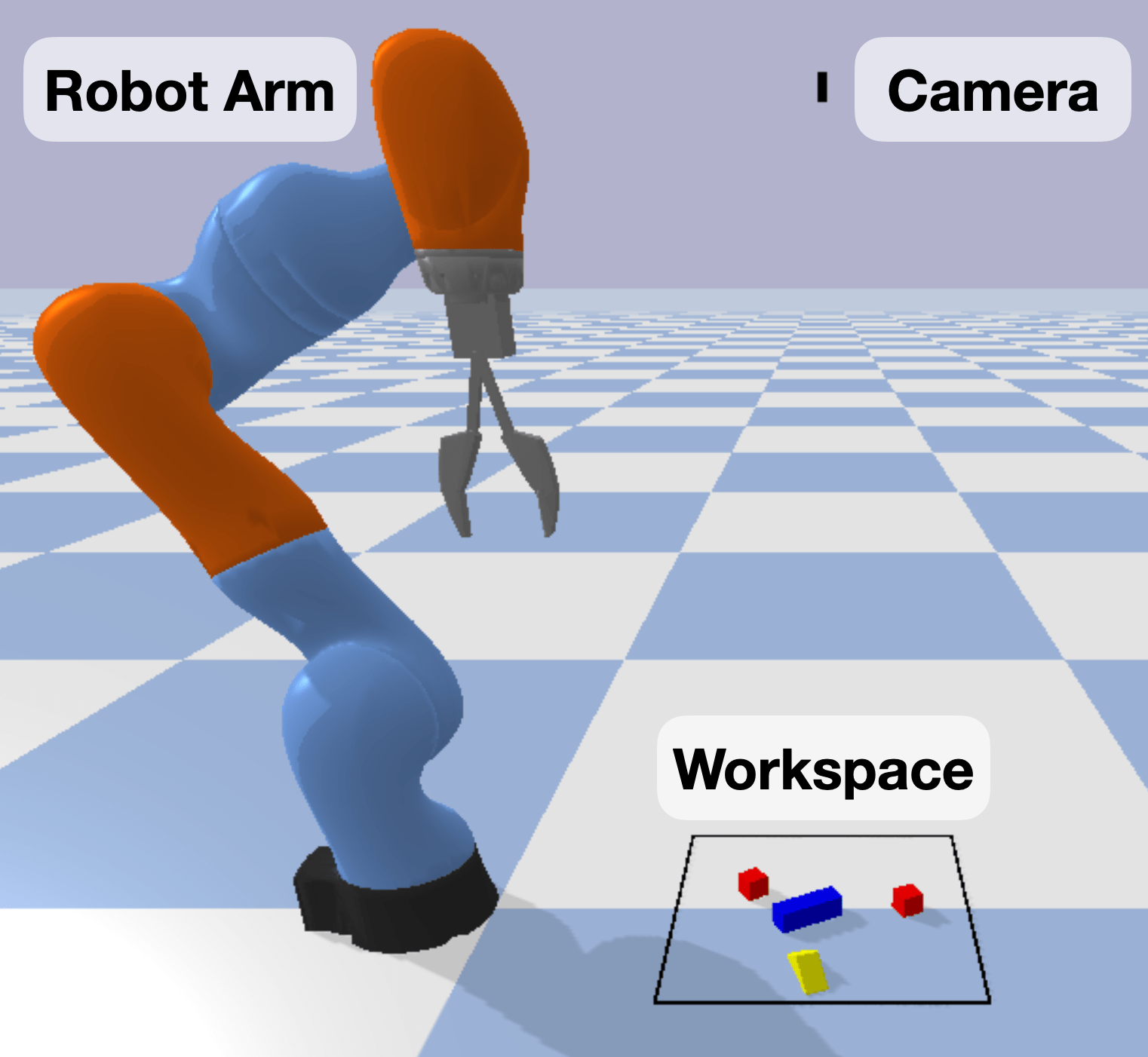
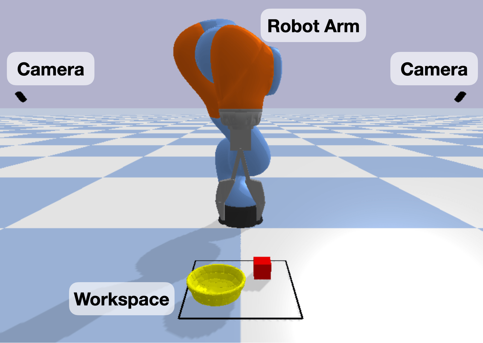
Our simulation setup (Figure 5) consists of a robot arm mounted on the floor of the simulation environment, a workspace in front of the robot where objects are generated, and a sensor. Typically, we use top-down sensors which generate heightmaps of the workspace. As we restrict the perception data to only the defined workspace, we choose to not add unnecessary elements to the setup such as a table for the arm to sit upon. Currently there are four different robot arms available in BulletArm (Figure 3): KUKA IIWA, Frane Emika Panda, Universal Robots UR5 with either a simple parallel jaw gripper or the Robotiq 2F-85 gripper.
Environment, Configuration, and Episode are three key terms within our framework. An environment is an instance of the PyBullet simulator in which the robot interacts with objects while trying to solve some task. This includes the initial environment state, the reward function, and termination requirements. A configuration contains additional specifications for the task such as the robotic arm, the size of the workspace, the physics mode, etc (see Appendix B for an full list of parameters). Episodes are generated by taking actions (steps) within an environment until the episode ends. An episode trajectory contains a series of observations , actions , and rewards : .
Users interface with the learning environment through the EnvironmentFactory and EnvironmentRunner classes. The EnvironmentFactory is the entry point and creates the Environment class specified by the Configuration passed as input. The EnvironmentFactory can create either a single environment or multiple environmaents meant to be run in parallel. In either case, an EnvironmentRunner instance is returned and provides the API which interacts with the environments. This API, Figure 1, is modelled after the typical agent-environment RL setup popularized by OpenAI Gym [4].
The benchmark tasks we provide have a sparse reward function which returns on successful task completion and otherwise. While we find this reward function to be advantageous as it avoids problems due to reward shaping, we do not require that new tasks conform to this. When defining a new task, the reward function defaults to sparse but users can easily define their custom reward for a new task. We separate our tasks into two categories based on the action spaces: open-loop control and closed-loop control. These two control modes are commonly used in robotics manipulation research.
3.3 Expert Demonstrations
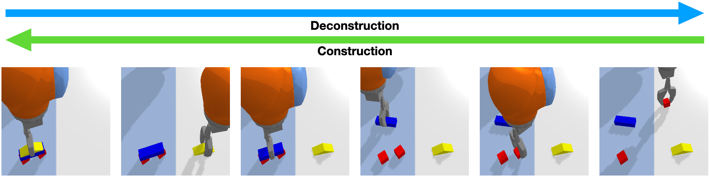
Expert demonstrations are crucial to many robotic learning fields. Methods such as imitation and model-based learning, for example, learn directly from expert demonstrations. Additionally, we find that in the context of reinforcement learning, it is vital to seed learning with expert demonstrations due to the difficulties in exploring large state-action spaces. We provide two types of planners to facilitate expert data generation: the Waypoint Planner and the Deconstruction Planner.
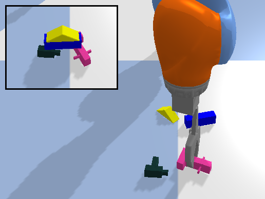
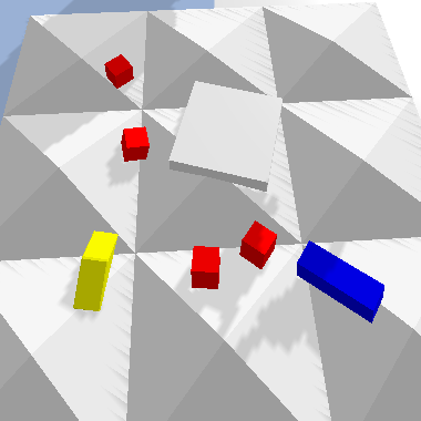
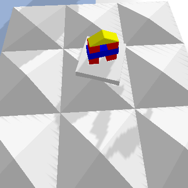
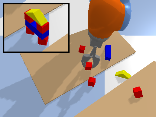
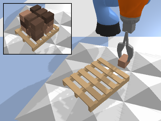
The Waypoint Planner is a online planning method which moves the end-effector through a series of waypoints in the workspace. We define a waypoint as where is the desired pose of the end effector and is the action primitive to execute at that pose. These waypoints can either be absolute positions in the workspace or positions relative to the objects in the workspace. In open-loop control, the planner returns the waypoint as the action executed at time . In close-loop control, the planner will continuously return a small displacement from the current end-effector pose as the action at time . This process is repeated until the waypoint has been reached. The Deconstruction Planner is a more limited planning method which can only be applied to pick-and-place tasks where the goal is to arrange objects in a specific manner. For example, we utilize this planner for the various block construction tasks examined in this work (Figure 2). When using this planner, the workspace is initialized with the objects in their target configuration and objects are then removed one-by-one until the initial state of the task is reached. This deconstruction trajectory, is then reversed to produce an expert construction trajectory, .
4 Environments
The core of any good benchmark is its set of environments. In robotic manipulation, in particular, it is important to cover a broad range of task difficulty and diversity. To this end, we introduce tasks covering a variety of skills for both open-loop and close-loop control. Moreover, the configurable parameters of our environments enable the user to select different task variations (e.g., the user can select whether the objects in the workspace will be initialized with a random orientation). BulletArm currently provides a collection of 21 open-loop manipulation environments and a collection of 10 close-loop environments. These environments are limited to kinematic tasks where the robot has to directly manipulate a collection of objects in order to reach some desired configuration.
4.1 Open-Loop Environments
Building 2
Building 3
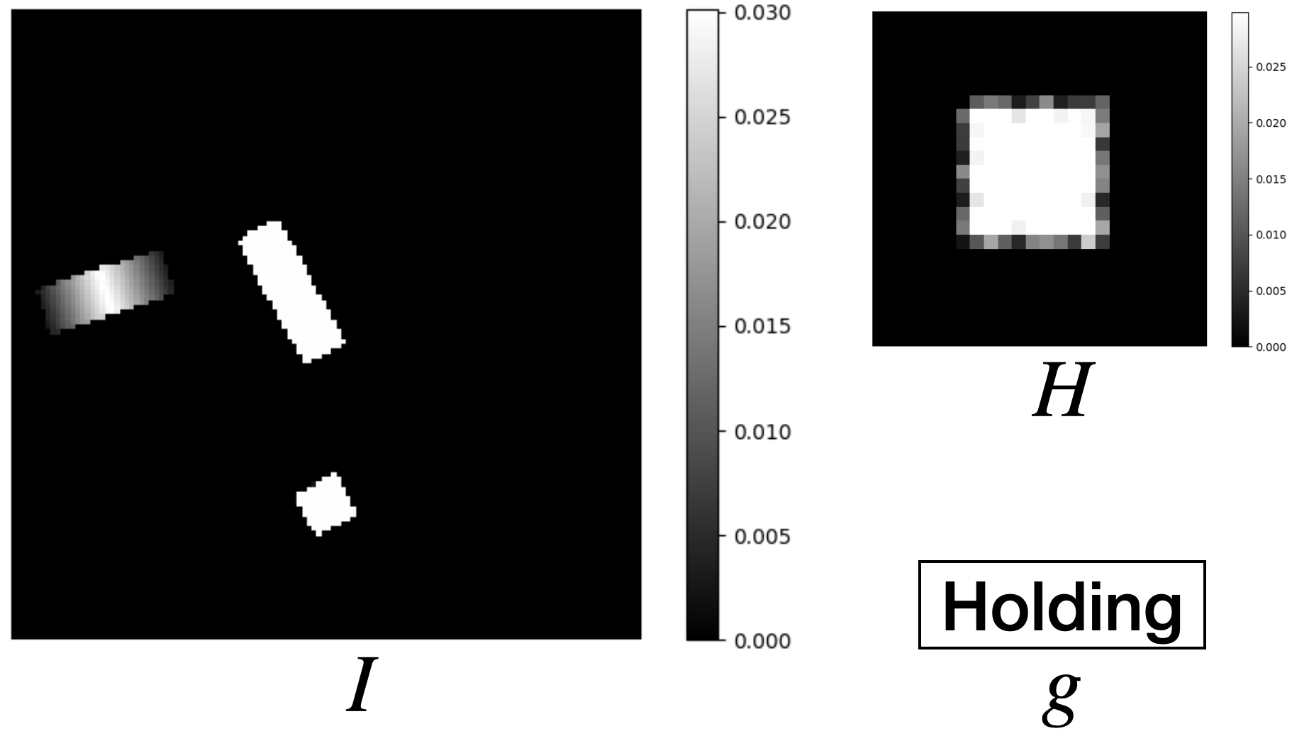
In the open-loop environments, the agent controls the target pose of the end-effector, resulting in a shorter time horizon for complex tasks. The open-loop environment is comprised of a robot arm, a workspace, and a camera above the workspace providing the observation (Figure 5). The action space is defined as the cross product of the gripper motion and the target pose of the gripper for that motion , . The state space is defined as (Figure 5), where is a top-down heightmap of the workspace; denotes the gripper state; and is an in-hand image that shows the object currently being held. If the last action is pick, then is a crop of the heightmap in the previous time step centered at the pick position. If the last action is place, is set to a zero value image.
BulletArm provides three different action spaces for : . The first option only controls the components of the gripper pose, where the rotation of the gripper is fixed; and is selected using a heuristic function that first reads the maximal height in the region around and then either adds a positive offset for a place action or a negative offset for pick action. The second option adds control of the rotation along the -axis. The third option controls the full 6 degree of freedom pose of the gripper, including the rotation along the -axis and the rotation along the -axis . and are suited for tasks that only require top-down manipulations, while is designed for solving complex tasks involving out-of-plane rotations. The definition of the state space and the action space in the open-loop environments also enables effortless sim2real transfer. One can reproduce the observation in Figure 5 in the real-world using an overhead depth camera and transfer the learned policy [43, 45].
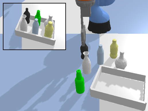
Figure 6 shows the 12 basic open-loop environments that can be solved using top-down actions. Those environments can be categorized into two collections, a set of block structure tasks (Figures 6a-6g), and a set of more realistic tasks (Figures 6h and 6l). The block structure tasks require the robot to build different goal structures using blocks. The more realistic tasks require the robot to finish some real-world problems, for example, arranging bottles or supervising Covid tests. We use the default sparse reward function for all open-loop environments, i.e., +1 reward for reaching the goal, and 0 otherwise. See Appendix A.1 for a detailed description of the tasks.
4.1.1 6DoF Extensions
The environments that we have introduced so far only require the robot to perform top-down manipulation. We extend those environments to 6 degrees of freedom by initializing them in either the ramp environment or the bump environment (Figure 7). In both cases, the robot needs to control the out-of-plane orientations introduced by the ramp or bump in order to manipulate the objects. We provide seven ramp environments (for each of the block structure construction tasks), and two bump environments (House Building 4 and Box Palletizing). See Appendix C for details.
4.2 Close-loop Environments
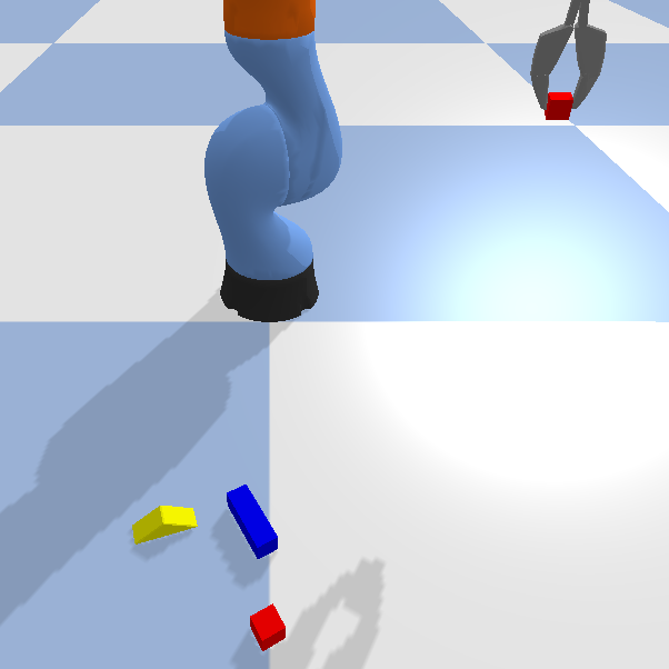
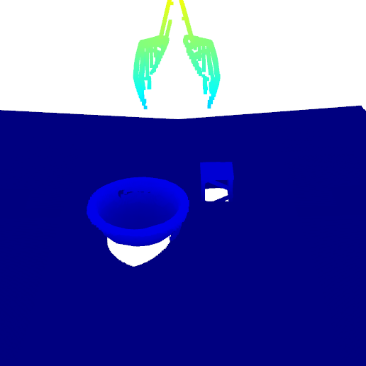
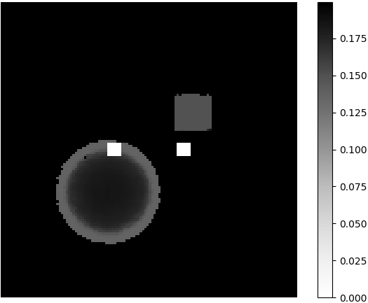
The close-loop environments require the agent to control the delta pose of the end-effector, allowing the agent more control and enabling us to solve more contact-rich tasks. These environments have a similar setup to the open-loop domain but to avoid the occlusion caused by the arm, we instead use two side-view cameras pointing to the workspace (Figure 8a). The heightmap is generated by first acquiring a fused point cloud from the two cameras (Figure 8b) and then performing an orthographic projection (Figure 8c). This orthographic projection is centered with respect to the gripper. In practice, this process can be replaced by putting a simulated orthographic camera at the position of the gripper to speed up the simulation. The state space is defined as a tuple , where is the gripper state indicating if there is an object being held by gripper. The action space is defined as the cross product of the gripper open width and the delta motion of the gripper , .
Two different action spaces are available for : . In , the robot controls the change of the position of the gripper, where the top-down orientation is fixed. In , the robot controls the change of the position and the top-down orientation of the gripper. Figure 9 shows the 10 close-loop environments. We provide a default sparse reward function for all environments. See Appendix A.2 for a detailed description of the tasks.
5 Benchmark
BulletArm provides a set of 5 benchmarks covering the various environments and action spaces (Table 1). In this section, we detail the Open-Loop 3D Benchmark and the Close-Loop 4D Benchmark. See Appendix D for the other three benchmarks.
| Benchmark | Environments | Action Space |
| Open-Loop 2D Benchmark | open-loop environments with fixed orientation | |
| Open-Loop 3D Benchmark | open-loop environments with random orientation | |
| Open-Loop 6D Benchmark | open-loop environments 6DoF extensions | |
| Close-Loop 3D Benchmark | close-loop environments with fixed orientation | |
| Close-Loop 4D Benchmark | close-loop environments with random orientation |
| Task |
Block Stacking |
House Building 1 |
House Building 2 |
House Building 3 |
House Building 4 |
Improvise House Building 2 |
Improvise House Building 3 |
Bin Packing |
Bottle Arrangement |
Box Palletizing |
Covid Test |
Object Grasping |
| Number of Objects | 4 | 4 | 3 | 4 | 6 | 3 | 4 | 8 | 6 | 18 | 6 | 15 |
| Optimal Number of Steps | 6 | 6 | 4 | 6 | 10 | 4 | 6 | 16 | 12 | 36 | 18 | 1 |
| Max Number of Steps | 10 | 10 | 10 | 10 | 20 | 10 | 10 | 20 | 20 | 40 | 30 | 1 |
5.1 Open-Loop 3D Benchmark
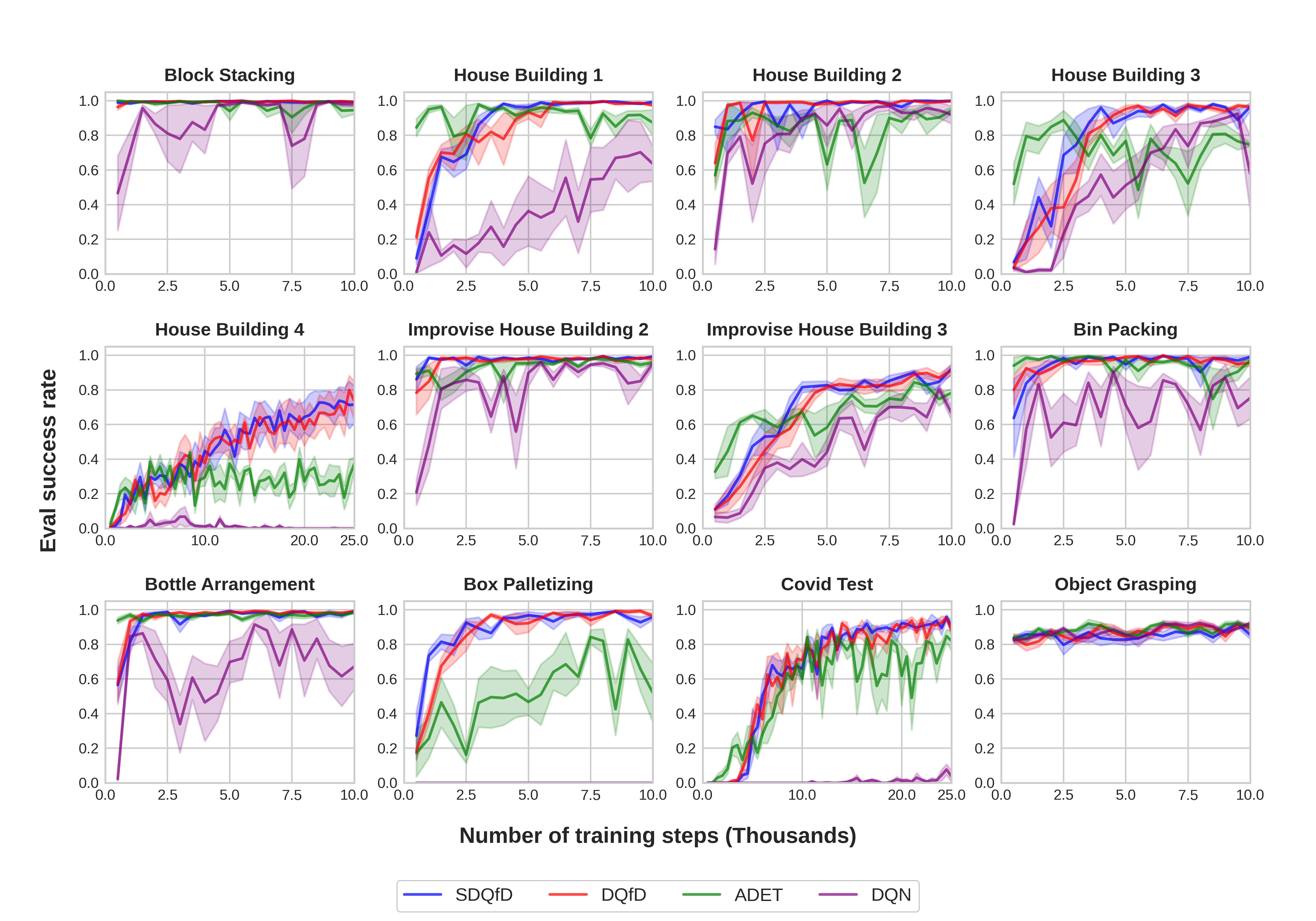
In the Open-Loop 3D Benchmark, the agent needs to solve the open-loop tasks shown in Figure 6 using the action space (see Section 4.1). We provide a set of baseline algorithms that explicitly control and select the gripper motion using the following heuristic: a pick action will be executed if and a place action will be executed if . The baselines include: (1) DQN [30], (2) ADET [24], (3) DQfD [15], and (4) SDQfD [43]. The network architectures for these different methods can be used interchangeably. We provide the following network architectures:
-
1.
CNN ASR [43]: A two-hierarchy architecture that selects and sequentially.
- 2.
-
3.
FCN: a Fully Convolutional Network (FCN) [29] which outputs a channel action-value map for each discrete rotation.
-
4.
Equivariant FCN [45]: Similar to FCN, but instead of using conventional CNNs, equivariant steerable CNNs are used.
- 5.
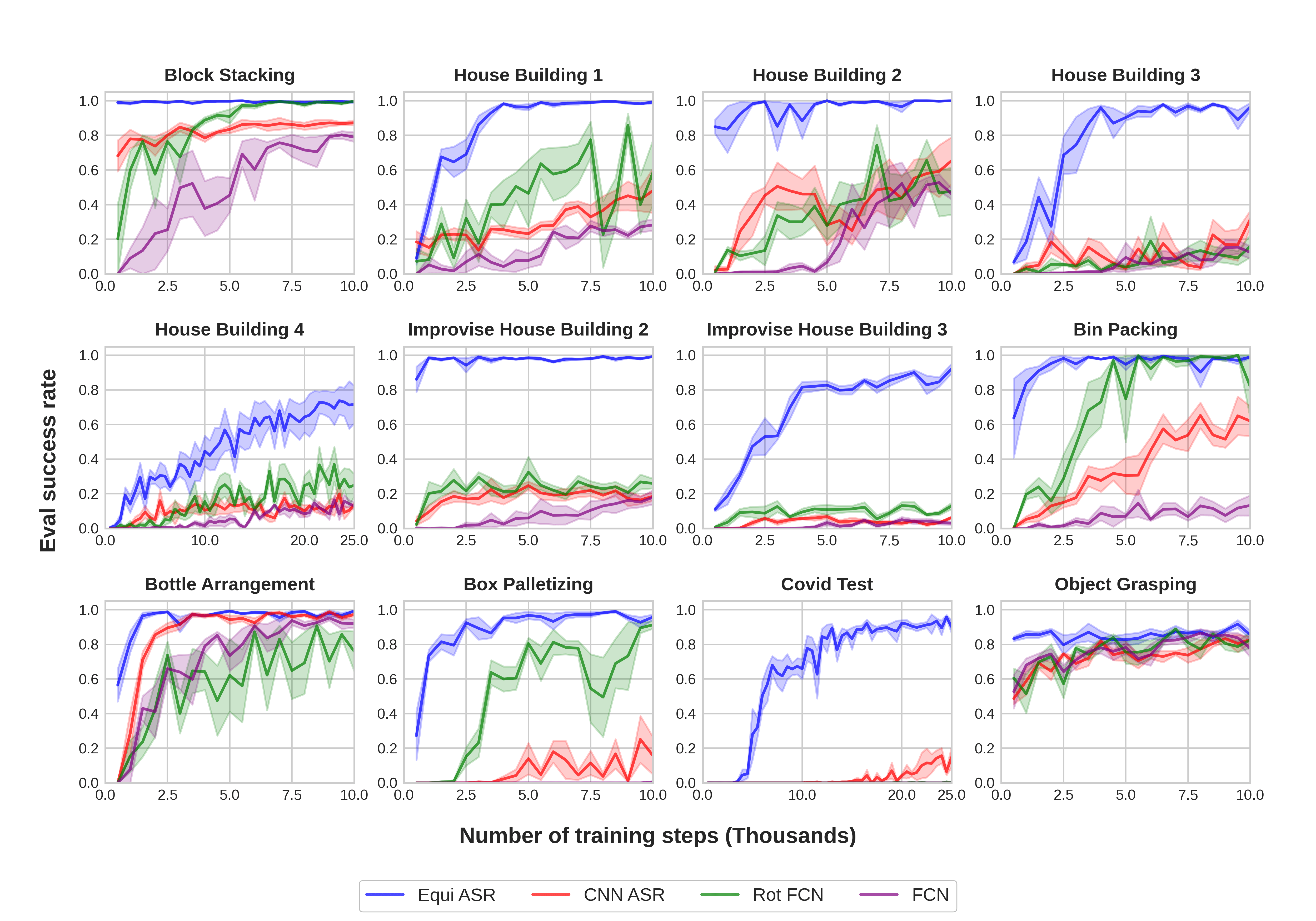
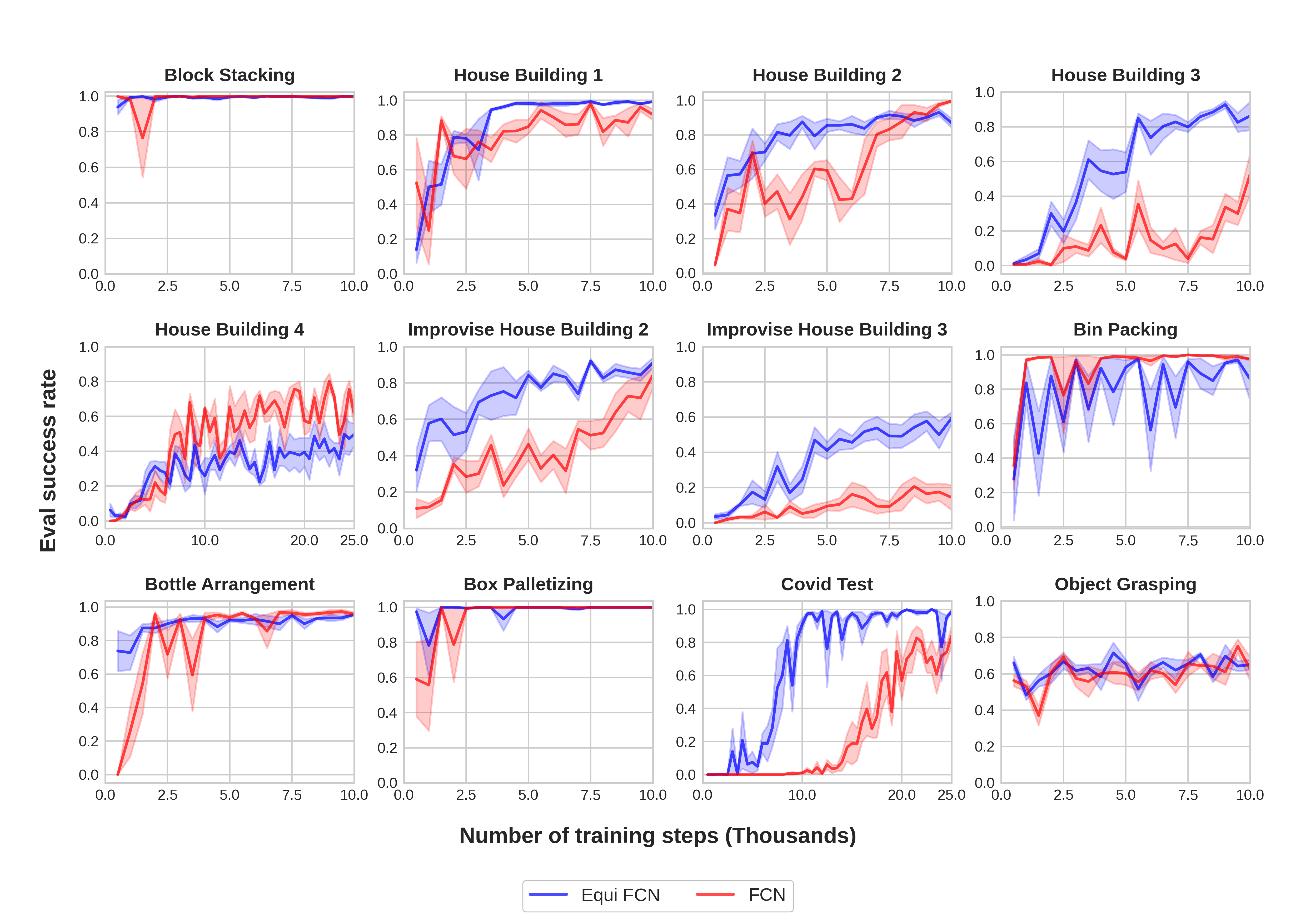
In this section, we show the performance of SDQfD (which is shown to be better than DQN, ADET, and DQfD [43]. See the performance of DQN, ADET and DQfD in Appendix E) equipped with CNN ASR, Equi ASR, FCN, and Rot FCN. We evaluate SDQfD in the 12 environments shown in Figure 6. Table 2 shows the number of objects, the optimal number of steps per episode, and the max number of steps per episode in the open-loop benchmark experiments. Before the start of training, 200 (500 for Covid Test) episodes of expert data are populated in the replay buffer. Figure 10 shows the results. Equivariant ASR (blue) has the best performance across all environments, then Rot FCN (green) and CNN ASR (red), and finally FCN (purple). Notice that Equivariant ASR is the only method that is capable of solving the most challenging tasks (e.g., Improvise House Building 3 and Covid Test).
5.2 Close-Loop 4D Benchmark
| Task |
Block Reaching |
Block Picking |
Block Pushing |
Block Pulling |
Block in Bowl |
Block Stacking |
House Building |
Corner Picking |
Drawer Opening |
Object Grasping |
| Number of Objects | 1 | 1 | 1 | 2 | 2 | 2 | 2 | 1 | 1 | 5 |
| Optimal Number of Steps | 3 | 7 | 7 | 7 | 11 | 12 | 12 | 14 | 9 | 7 |
| Max Number of Steps | 50 | 50 | 50 | 50 | 50 | 50 | 50 | 50 | 50 | 50 |
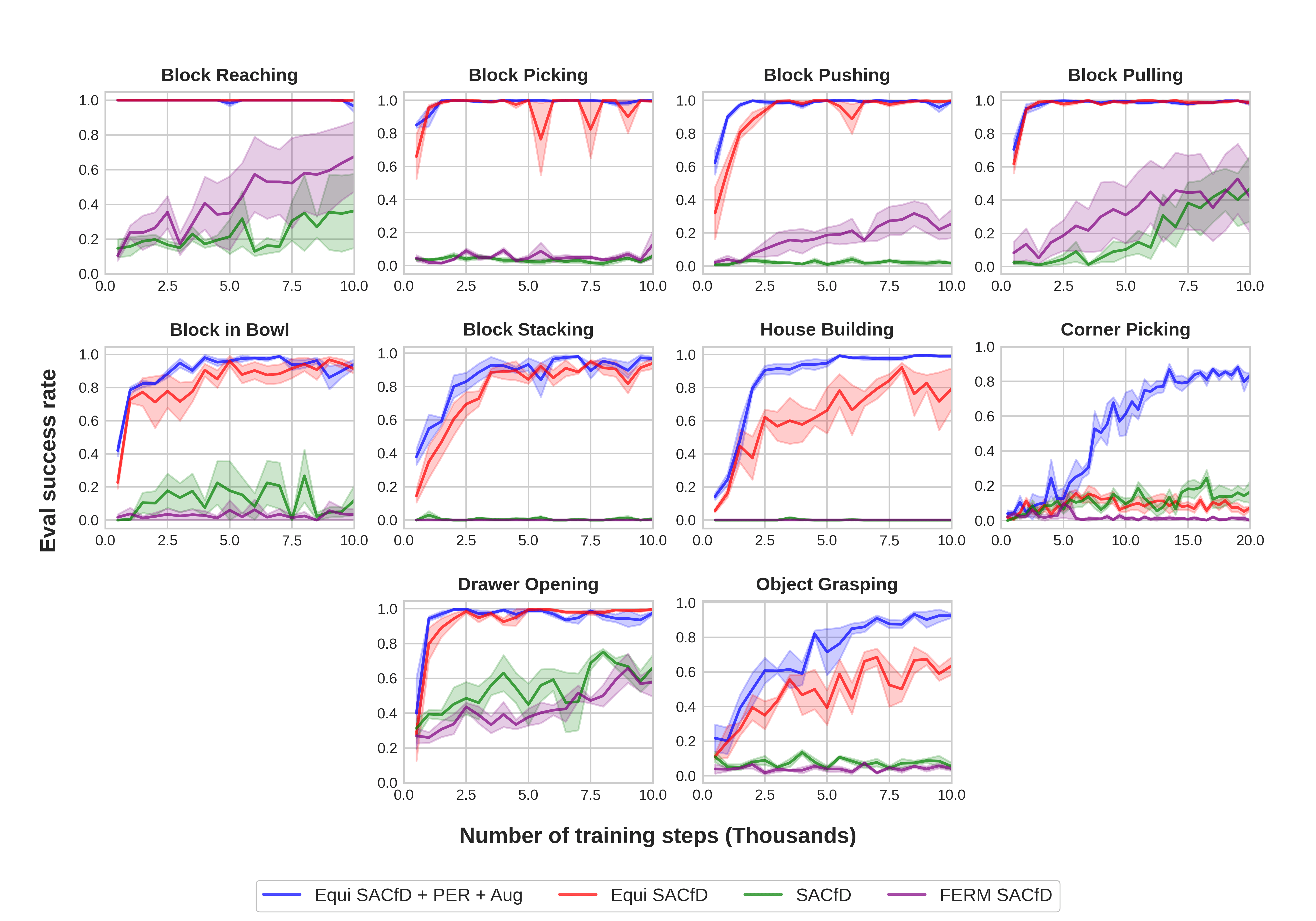
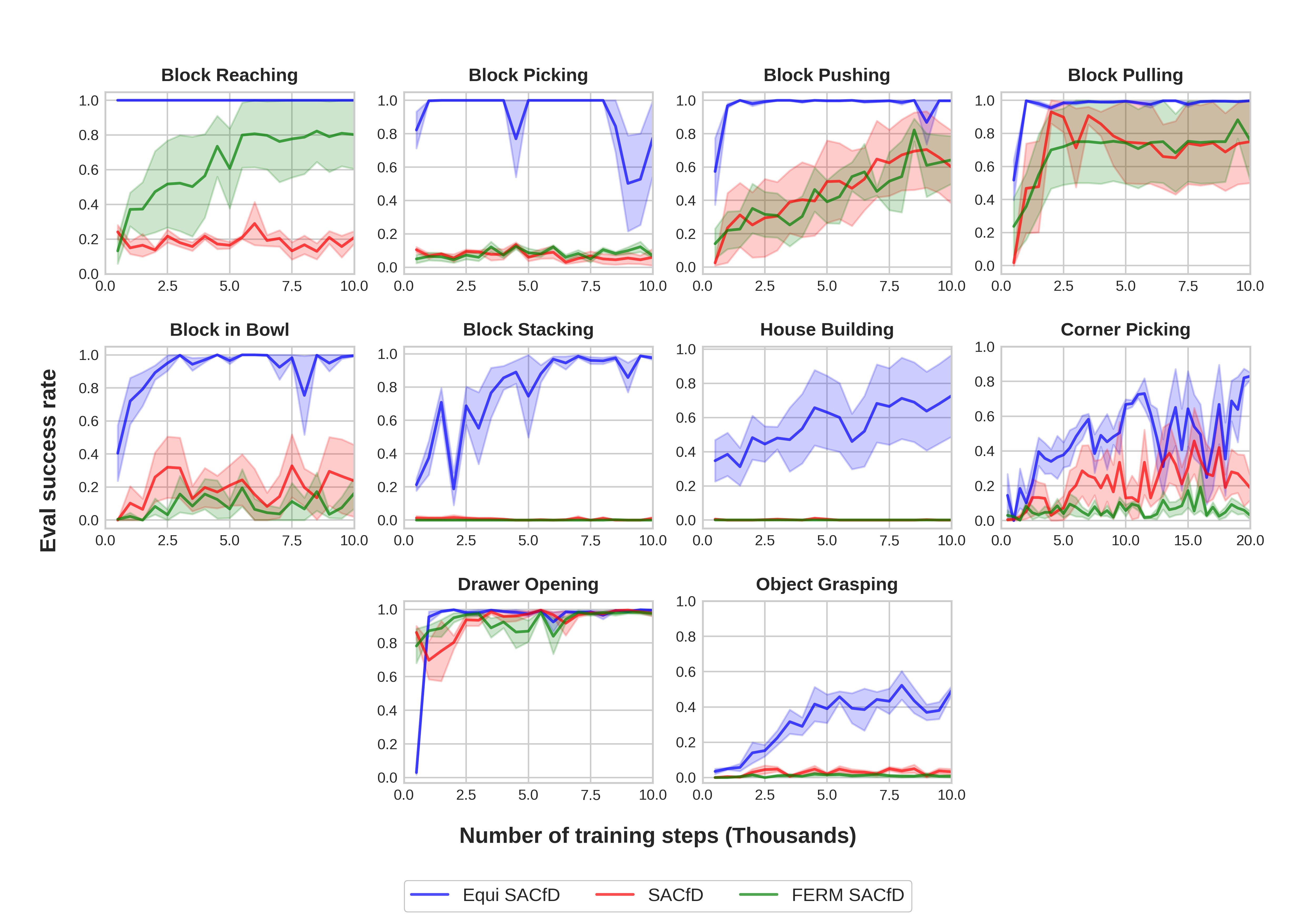
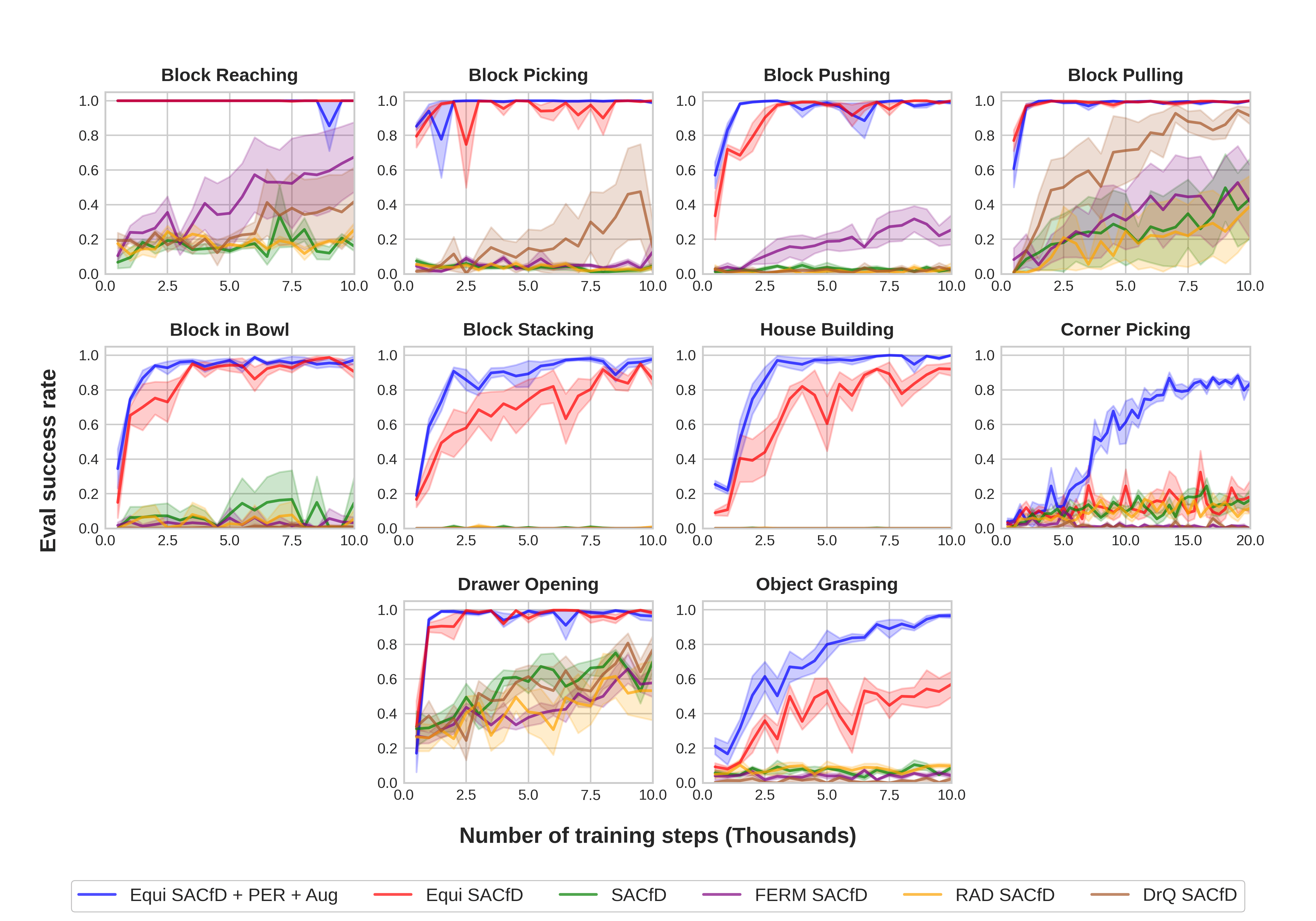
The Close-Loop 4D Benchmark requires the agent to solve the close-loop tasks shown in Figure 9 in the 5-dimensional action space of , where the agent controls the positional displacement of the gripper (), the rotational displacement of the gripper along the axis (), and the open width of the gripper (). We provide the following baseline algorithms: (1) SAC [13], (2) Equivariant SAC [44], (3) RAD [25] SAC: SAC with data augmentation, (4) DrQ [23] SAC: Similar to (3), but performs data augmentation when calculating the -target and the loss, and (5) FERM [53]: A Combination of SAC and contrastive learning [26] using data augmentation. Additionally, we also provide a variation of SAC, SACfD [44], that applies an auxiliary L2 loss towards the expert action to the actor network. SACfD can also be used in combination with (2), (3), and (4) to form Equivariant SACfD, RAD SACfD, DrQ SACfD, and FERM SACfD.
In this section, we show the performance of SACfD, Equivariant SACfD (Equi SACfD), Equivariant SACfD using Prioritized Experience Replay (PER [35]) and data augmentation (Equi SACfD + PER + Aug), and FERM SACfD. (See Appendix F for the performance of RAD SACfD and DrQ SACfD.) We use a continuous action space where . We evaluate the various methods in the 10 environments shown in Figure 9. Table 3 shows the number of objects, the optimal number of steps for solving each task, and the maximal number of steps for each episode. In all tasks, we pre-load 100 episodes of expert demonstrations in the replay buffer.
Figure 11 shows the performance of the baselines. Equivariant SACfD with PER and data augmentation (blue) has the best overall performance followed by standard Equivariant SACfD (red). The equivariant algorithms show a significant improvement when compared to the other algorithms which do not encode rotation symmetry, i.e. CNN SACfD and FERM SACfD.
6 Conclusions
In this paper, we present BulletArm, a novel benchmark and learning environment aimed at robotic manipulation. By providing a number of manipulation tasks alongside our baseline algorithms, we hope to encourage more direct comparisons between new methods. This type of standardization through direct comparison has been a key aspect of improving research in deep learning methods for both computer vision and reinforcement learning. We aim to maintain and improve this framework for the foreseeable future adding new features, tasks, and baseline algorithms over time. An area of particular interest for us is to extend the existing suite of tasks to include more dynamic environments where the robot is tasked with utilizing tools to accomplish various tasks. We hope that with the aid of the community, this repository will grow over time to contain both a large number of interesting tasks and state-of-the-art baseline algorithms.
Acknowledgments
This work is supported in part by NSF 1724257, NSF 1724191, NSF 1763878, NSF 1750649, and NASA 80NSSC19K1474.
References
- [1] O. M. Andrychowicz, B. Baker, M. Chociej, R. Jozefowicz, B. McGrew, J. Pachocki, A. Petron, M. Plappert, G. Powell, A. Ray, et al. Learning dexterous in-hand manipulation. The International Journal of Robotics Research, 39(1):3–20, 2020.
- [2] M. G. Bellemare, Y. Naddaf, J. Veness, and M. Bowling. The arcade learning environment: An evaluation platform for general agents. Journal of Artificial Intelligence Research, 47:253–279, 2013.
- [3] O. Biza, D. Wang, R. Platt, J.-W. van de Meent, and L. L. Wong. Action priors for large action spaces in robotics. In Proceedings of the 20th International Conference on Autonomous Agents and MultiAgent Systems, pages 205–213, 2021.
- [4] G. Brockman, V. Cheung, L. Pettersson, J. Schneider, J. Schulman, J. Tang, and W. Zaremba. Openai gym. arXiv preprint arXiv:1606.01540, 2016.
- [5] T. S. Cohen and M. Welling. Steerable cnns. arXiv preprint arXiv:1612.08498, 2016.
- [6] E. Coumans and Y. Bai. Pybullet, a python module for physics simulation for games, robotics and machine learning. GitHub repository, 2016.
- [7] B. Delhaisse, L. D. Rozo, and D. G. Caldwell. Pyrobolearn: A python framework for robot learning practitioners. In CoRL, 2019.
- [8] J. Deng, W. Dong, R. Socher, L.-J. Li, K. Li, and L. Fei-Fei. Imagenet: A large-scale hierarchical image database. In 2009 IEEE conference on computer vision and pattern recognition, pages 248–255. Ieee, 2009.
- [9] A. Depierre, E. Dellandréa, and L. Chen. Jacquard: A large scale dataset for robotic grasp detection. In 2018 IEEE/RSJ International Conference on Intelligent Robots and Systems (IROS), pages 3511–3516. IEEE, 2018.
- [10] C. Devin, A. Gupta, T. Darrell, P. Abbeel, and S. Levine. Learning modular neural network policies for multi-task and multi-robot transfer. In 2017 IEEE international conference on robotics and automation (ICRA), pages 2169–2176. IEEE, 2017.
- [11] H.-S. Fang, C. Wang, M. Gou, and C. Lu. Graspnet-1billion: A large-scale benchmark for general object grasping. In Proceedings of the IEEE/CVF Conference on Computer Vision and Pattern Recognition, pages 11444–11453, 2020.
- [12] S. Gu, E. Holly, T. Lillicrap, and S. Levine. Deep reinforcement learning for robotic manipulation with asynchronous off-policy updates. In 2017 IEEE international conference on robotics and automation (ICRA), pages 3389–3396. IEEE, 2017.
- [13] T. Haarnoja, A. Zhou, K. Hartikainen, G. Tucker, S. Ha, J. Tan, V. Kumar, H. Zhu, A. Gupta, P. Abbeel, et al. Soft actor-critic algorithms and applications. arXiv preprint arXiv:1812.05905, 2018.
- [14] K. Hausman, J. T. Springenberg, Z. Wang, N. Heess, and M. Riedmiller. Learning an embedding space for transferable robot skills. In International Conference on Learning Representations, 2018.
- [15] T. Hester, M. Vecerik, O. Pietquin, M. Lanctot, T. Schaul, B. Piot, D. Horgan, J. Quan, A. Sendonaris, I. Osband, et al. Deep q-learning from demonstrations. In Thirty-Second AAAI Conference on Artificial Intelligence, 2018.
- [16] P. J. Huber. Robust estimation of a location parameter. The Annals of Mathematical Statistics, 35(1):73–101, 1964.
- [17] S. James, M. Freese, and A. J. Davison. Pyrep: Bringing v-rep to deep robot learning. arXiv preprint arXiv:1906.11176, 2019.
- [18] S. James, Z. Ma, D. R. Arrojo, and A. J. Davison. Rlbench: The robot learning benchmark & learning environment. IEEE Robotics and Automation Letters, 5(2):3019–3026, 2020.
- [19] Y. Jiang, S. Moseson, and A. Saxena. Efficient grasping from rgbd images: Learning using a new rectangle representation. In 2011 IEEE International conference on robotics and automation, pages 3304–3311. IEEE, 2011.
- [20] D. Kalashnikov, A. Irpan, P. Pastor, J. Ibarz, A. Herzog, E. Jang, D. Quillen, E. Holly, M. Kalakrishnan, V. Vanhoucke, et al. Scalable deep reinforcement learning for vision-based robotic manipulation. In Conference on Robot Learning, pages 651–673. PMLR, 2018.
- [21] M. Kempka, M. Wydmuch, G. Runc, J. Toczek, and W. Jaśkowski. Vizdoom: A doom-based ai research platform for visual reinforcement learning. In 2016 IEEE conference on computational intelligence and games (CIG), pages 1–8. IEEE, 2016.
- [22] D. P. Kingma and J. Ba. Adam: A method for stochastic optimization. arXiv preprint arXiv:1412.6980, 2014.
- [23] I. Kostrikov, D. Yarats, and R. Fergus. Image augmentation is all you need: Regularizing deep reinforcement learning from pixels. arXiv preprint arXiv:2004.13649, 2020.
- [24] A. S. Lakshminarayanan, S. Ozair, and Y. Bengio. Reinforcement learning with few expert demonstrations. In NIPS Workshop on Deep Learning for Action and Interaction, volume 2016, 2016.
- [25] M. Laskin, K. Lee, A. Stooke, L. Pinto, P. Abbeel, and A. Srinivas. Reinforcement learning with augmented data. Advances in Neural Information Processing Systems, 33:19884–19895, 2020.
- [26] M. Laskin, A. Srinivas, and P. Abbeel. Curl: Contrastive unsupervised representations for reinforcement learning. In International Conference on Machine Learning, pages 5639–5650. PMLR, 2020.
- [27] Y. Lee, E. Hu, Z. Yang, A. C. Yin, and J. J. Lim. Ikea furniture assembly environment for long-horizon complex manipulation tasks. 2021 IEEE International Conference on Robotics and Automation (ICRA), pages 6343–6349, 2021.
- [28] R. Li, A. Jabri, T. Darrell, and P. Agrawal. Towards practical multi-object manipulation using relational reinforcement learning. In 2020 IEEE International Conference on Robotics and Automation (ICRA), pages 4051–4058. IEEE, 2020.
- [29] J. Long, E. Shelhamer, and T. Darrell. Fully convolutional networks for semantic segmentation. In Proceedings of the IEEE conference on computer vision and pattern recognition, pages 3431–3440, 2015.
- [30] V. Mnih, K. Kavukcuoglu, D. Silver, A. A. Rusu, J. Veness, M. G. Bellemare, A. Graves, M. Riedmiller, A. K. Fidjeland, G. Ostrovski, et al. Human-level control through deep reinforcement learning. nature, 518(7540):529–533, 2015.
- [31] A. Nair, B. McGrew, M. Andrychowicz, W. Zaremba, and P. Abbeel. Overcoming exploration in reinforcement learning with demonstrations. In 2018 IEEE international conference on robotics and automation (ICRA), pages 6292–6299. IEEE, 2018.
- [32] A. Paszke, S. Gross, S. Chintala, G. Chanan, E. Yang, Z. DeVito, Z. Lin, A. Desmaison, L. Antiga, and A. Lerer. Automatic differentiation in PyTorch. In NIPS Autodiff Workshop, 2017.
- [33] P. Rohlfshagen and S. M. Lucas. Ms pac-man versus ghost team cec 2011 competition. In 2011 IEEE Congress of Evolutionary Computation (CEC), pages 70–77. IEEE, 2011.
- [34] E. Rohmer, S. P. Singh, and M. Freese. V-rep: A versatile and scalable robot simulation framework. In 2013 IEEE/RSJ International Conference on Intelligent Robots and Systems, pages 1321–1326. IEEE, 2013.
- [35] T. Schaul, J. Quan, I. Antonoglou, and D. Silver. Prioritized experience replay. arXiv preprint arXiv:1511.05952, 2015.
- [36] D. Silver, A. Huang, C. J. Maddison, A. Guez, L. Sifre, G. Van Den Driessche, J. Schrittwieser, I. Antonoglou, V. Panneershelvam, M. Lanctot, et al. Mastering the game of go with deep neural networks and tree search. nature, 529(7587):484–489, 2016.
- [37] Y. Tassa, Y. Doron, A. Muldal, T. Erez, Y. Li, D. d. L. Casas, D. Budden, A. Abdolmaleki, J. Merel, A. Lefrancq, et al. Deepmind control suite. arXiv preprint arXiv:1801.00690, 2018.
- [38] E. Todorov, T. Erez, and Y. Tassa. Mujoco: A physics engine for model-based control. In 2012 IEEE/RSJ international conference on intelligent robots and systems, pages 5026–5033. IEEE, 2012.
- [39] J. Togelius, S. Karakovskiy, and R. Baumgarten. The 2009 mario ai competition. In IEEE Congress on Evolutionary Computation, pages 1–8. IEEE, 2010.
- [40] Y. Urakami, A. Hodgkinson, C. Carlin, R. Leu, L. Rigazio, and P. Abbeel. Doorgym: A scalable door opening environment and baseline agent. ArXiv, abs/1908.01887, 2019.
- [41] O. Vinyals, T. Ewalds, S. Bartunov, P. Georgiev, A. S. Vezhnevets, M. Yeo, A. Makhzani, H. Küttler, J. Agapiou, J. Schrittwieser, et al. Starcraft ii: A new challenge for reinforcement learning. arXiv preprint arXiv:1708.04782, 2017.
- [42] D. Wang, M. Jia, X. Zhu, R. Walters, and R. Platt. On-robot policy learning with -equivariant sac. arXiv preprint arXiv:2203.04923, 2022.
- [43] D. Wang, C. Kohler, and R. Platt. Policy learning in se (3) action spaces. In Conference on Robot Learning, pages 1481–1497. PMLR, 2021.
- [44] D. Wang, R. Walters, and R. Platt. -equivariant reinforcement learning. In International Conference on Learning Representations, 2022.
- [45] D. Wang, R. Walters, X. Zhu, and R. Platt. Equivariant learning in spatial action spaces. In Conference on Robot Learning, pages 1713–1723. PMLR, 2022.
- [46] M. Weiler and G. Cesa. General -equivariant steerable cnns. arXiv preprint arXiv:1911.08251, 2019.
- [47] W. Wohlkinger, A. Aldoma Buchaca, R. Rusu, and M. Vincze. 3DNet: Large-Scale Object Class Recognition from CAD Models. In IEEE International Conference on Robotics and Automation (ICRA), 2012.
- [48] T. Yu, D. Quillen, Z. He, R. Julian, K. Hausman, C. Finn, and S. Levine. Meta-world: A benchmark and evaluation for multi-task and meta reinforcement learning. In Conference on Robot Learning, pages 1094–1100. PMLR, 2020.
- [49] K. Zakka, A. Zeng, J. Lee, and S. Song. Form2fit: Learning shape priors for generalizable assembly from disassembly. In 2020 IEEE International Conference on Robotics and Automation (ICRA), pages 9404–9410. IEEE, 2020.
- [50] A. Zeng, P. Florence, J. Tompson, S. Welker, J. Chien, M. Attarian, T. Armstrong, I. Krasin, D. Duong, V. Sindhwani, et al. Transporter networks: Rearranging the visual world for robotic manipulation. In Conference on Robot Learning, pages 726–747. PMLR, 2021.
- [51] A. Zeng, S. Song, S. Welker, J. Lee, A. Rodriguez, and T. Funkhouser. Learning synergies between pushing and grasping with self-supervised deep reinforcement learning. In 2018 IEEE/RSJ International Conference on Intelligent Robots and Systems (IROS), pages 4238–4245. IEEE, 2018.
- [52] A. Zeng, S. Song, K.-T. Yu, E. Donlon, F. R. Hogan, M. Bauza, D. Ma, O. Taylor, M. Liu, E. Romo, et al. Robotic pick-and-place of novel objects in clutter with multi-affordance grasping and cross-domain image matching. In 2018 IEEE international conference on robotics and automation (ICRA), pages 3750–3757. IEEE, 2018.
- [53] A. Zhan, P. Zhao, L. Pinto, P. Abbeel, and M. Laskin. A framework for efficient robotic manipulation. arXiv preprint arXiv:2012.07975, 2020.
- [54] X. Zhu, D. Wang, O. Biza, G. Su, R. Walters, and R. Platt. Sample efficient grasp learning using equivariant models. Proceedings of Robotics: Science and Systems (RSS), 2022.
- [55] Y. Zhu, J. Wong, A. Mandlekar, and R. Mart’in-Mart’in. robosuite: A modular simulation framework and benchmark for robot learning. ArXiv, abs/2009.12293, 2020.
Appendix A Detail Description of Environments
A.1 Open-Loop Environments
A.1.1 Block Stacking
In the Block Stacking environment (Figure 6a), there are cubic blocks with a size of . The blocks are randomly initialized in the workspace. The goal of this task is to stack all blocks in a stack. An optimal policy requires steps to finish this task. The number of blocks is configurable. By default, , and the maximal number of steps per episode is 10.
A.1.2 House Building 1
In the House Building 1 environment (Figure 6b), there are cubic blocks with a size of and one triangle block with a bounding box size of around . The blocks are randomly initialized in the workspace. The goal of this task is to first form a stack using the cubic blocks, then place the triangle block on top of the stack. An optimal policy requires steps to finish this task. The number of blocks is configurable. By default, , and the maximal number of steps per episode is 10.
A.1.3 House Building 2
In the House Building 2 environment (Figure 6c), there are two cubic blocks with a size of , and a roof block with a bounding box size of around . The blocks are randomly initialized in the workspace. The goal of this task is to place the two cubic blocks next to each other, then place the roof block on top of the two cubic blocks. An optimal policy requires 4 steps to finish this task. The default maximal number of steps per episode is 10.
A.1.4 House Building 3
In the House Building 3 environment (Figure 6d), there are two cubic blocks with a size of , one cuboid block with a size of , and a roof block with a bounding box size of around . The blocks are randomly initialized in the workspace. The goal of this task is to first place the two cubic blocks next to each other, place the cuboid block on top of the two cubic blocks, then place the roof block on top of the cuboid block. An optimal policy requires 6 steps to finish this task. The default maximal number of steps per episode is 10.
A.1.5 House Building 4
In the House Building 4 environment (Figure 6e), there are four cubic blocks with a size of , one cuboid block with a size of , and a roof block with a bounding box size of around . The blocks are randomly initialized in the workspace. The goal of this task is to first place two cubic blocks next to each other, place the cuboid block on top of the two cubic blocks, place another two cubic blocks on top of the cuboid block, then place the roof block on top of the two cubic blocks. An optimal policy requires 10 steps to finish this task. The default maximal number of steps per episode is 20.
A.1.6 Improvise House Building 2
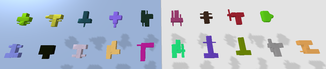
In the Improvise House Building 2 environment (Figure 6f), there are two random blocks and a roof block. The shapes of the random blocks are sampled from Figure 12. The blocks are randomly initialized in the workspace. The goal of this task is to place the two random blocks next to each other, then place the roof block on top of the two random blocks. An optimal policy requires 4 steps to finish this task. The default maximal number of steps per episode is 10.
A.1.7 Improvise House Building 3
In the Improvise House Building 3 environment (Figure 6g), there are two random blocks, a cuboid block, and a roof block. The shapes of the random blocks are sampled from Figure 12. The blocks are randomly initialized in the workspace. The goal of this task is to place the two random blocks next to each other, place the cuboid block on top of the two random blocks, then place the roof block on top of the cuboid block. An optimal policy requires 6 steps to finish this task. The default maximal number of steps per episode is 10.
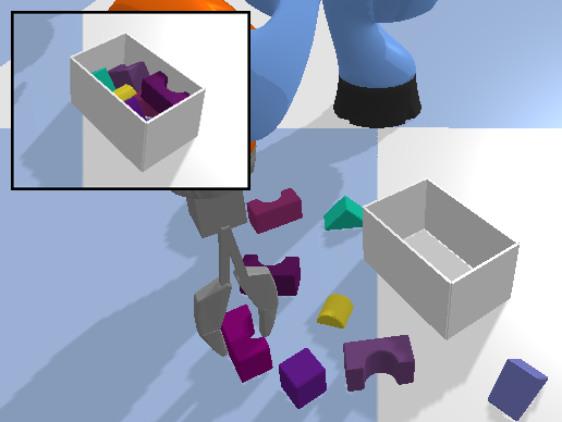
A.1.8 Bin Packing
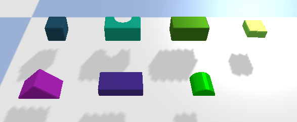
In the Bin Packing task (Figure 6h), objects and a bin are randomly placed in the workspace. The shapes of the objects are randomly sampled from Figure 13 (Object models are derived from [51]) with a maximum size of and a minimum size of . The bin has a size of . The goal of this task is to pack all objects in the bin. An optimal policy requires steps to finish the task. The number of objects is configurable. By default, , and the maximal number of steps per episode is 20.
A.1.9 Bottle Arrangement
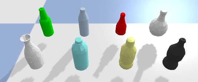
In the Bottle Arrangement task (Figure 6i), six bottles with random shapes (sampled from 8 different shapes shown in Figure 14. The bottle shapes are generated from the 3DNet dataset [47]. The sizes of each bottle are around ), and a tray with a size of are randomly placed in the workspace. The goal is to arrange all six bottles in the tray. An optimal policy requires 12 steps to finish this task. By default, the maximal number of steps per episode is 20.
A.1.10 Box Palletizing
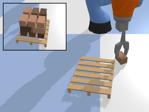
In the Box Palletizing task (Figure 6j) (some object models are derived from [50]), a pallet with a size of is randomly placed in the workspace. The goal is to stack boxes with a size of as shown in Fig 6j. At the beginning of each episode and after the agent correctly places a box on the pallet, a new box will be randomly placed in the empty workspace. An optimal policy requires steps to finish this task. The number of boxes is configurable (6, 12, or 18). By default, , and the maximal number of steps per episode is 40.
A.1.11 Covid Test
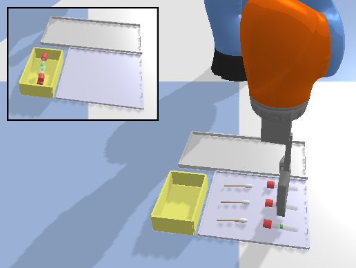
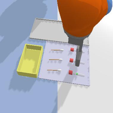
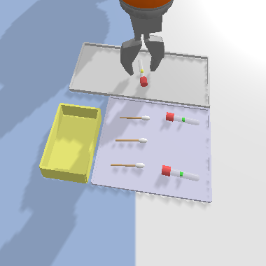
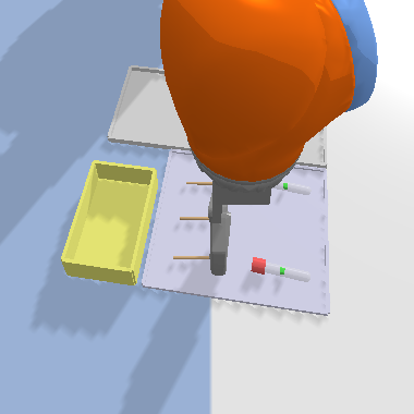
In the Covid Test task (Figure 6k), there is a new tube box (purple), a test area (gray), and a used tube box (yellow) placed arbitrarily in the workspace but adjacent to one another. Three swabs with a size of and three tubes with a size of are initialized in the new tube box. To supervise a COVID test, the robot needs to present a pair of a new swab and a new tube from the new tube box to the test area. The simulator simulates the user testing COVID by putting the swab into the tube and randomly placing the used tube in the test area. Then the robot needs to re-collect the used tube into the used tube box. See one example of this process in Figure 15. Each episode includes three rounds of COVID test. An optimal policy requires 18 steps to finish this task. By default, the maximal number of steps per episode is 30.
A.1.12 Object Grasping
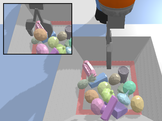
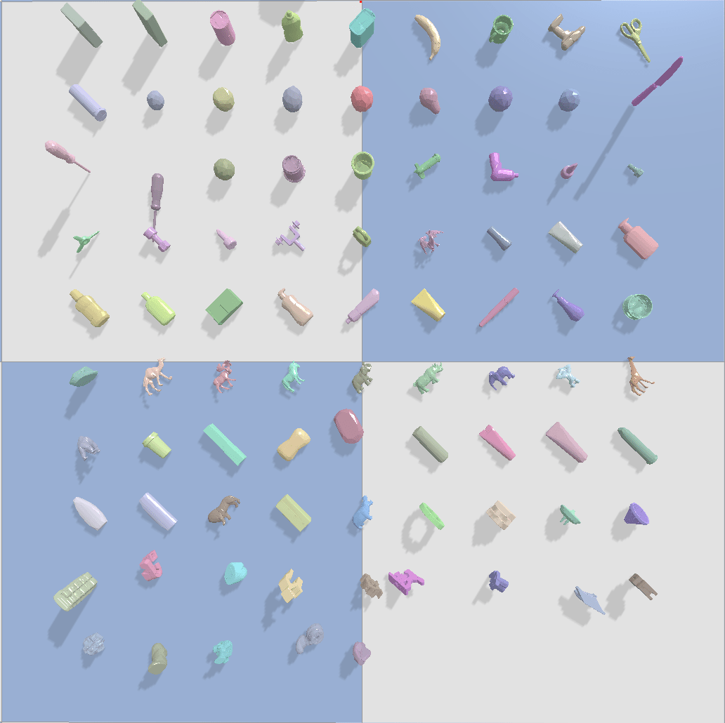
In the Object Grasping task (Figure 6l), the robot needs to grasp an object from a clutter of at most objects. At the start of training, random objects are initialized with random position and orientation. The shapes of the objects are randomly sampled from the object set shown in Figure 16. The object set contains 86 objects derived from the GraspNet1B [11] dataset. Every time the agent successfully grasps all objects, the environment will re-generate random objects with random positions and orientations. The maximal number of steps per episode is 1. The number of objects in this environment is configurable. By default, there will be 15 objects.
A.2 Close-Loop Environments
A.2.1 Block Reaching
In the Block Reaching environment (Figure 9a), there is a cubic block with a size of . The block is randomly initialized in the workspace. The goal of this task is to move the gripper towards the block such that the distance of the fingertip and the block is within . By default, the maximal number of steps per episode is 50.
A.2.2 Block Picking
In the Block Picking environment (Figure 9b), there is a cubic block with a size of . The block is randomly initialized in the workspace. The goal of this task is to grasp the block and raise the gripper such that the gripper is above the ground. By default, the maximal number of steps per episode is 50.
A.2.3 Block Pushing
In the Block Pushing environment (Figure 9c), there is a cubic block with a size of and a goal area with a size of . The block and the goal area are randomly initialized in the workspace. The goal of this task is to push the block such that the distance between the block’s center and the goal’s center is within . By default, the maximal number of steps per episode is 50.
A.2.4 Block Pulling
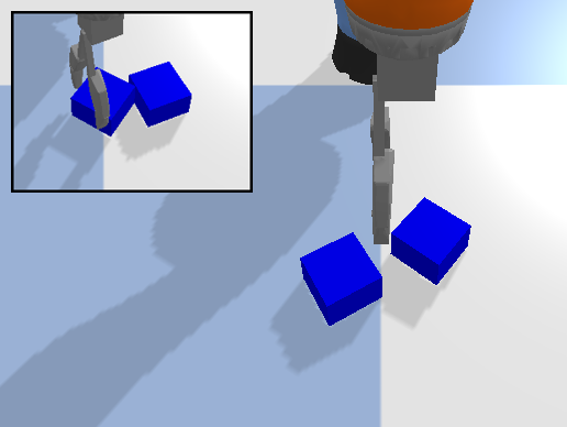
In the Block Pulling environment (Figure 9d), there are two cuboid blocks with a size of . The blocks are randomly initialized in the workspace. The goal of this task is to pull one of the two blocks such that it makes contact with another block. By default, the maximal number of steps per episode is 50.
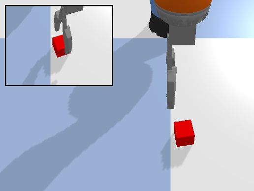
A.2.5 Block in Bowl
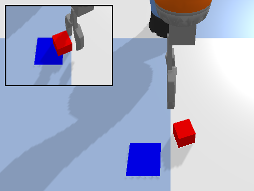
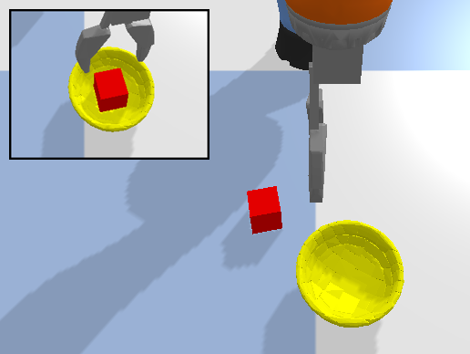
In the Block in Bowl environment (Figure 9e), there is a cubic block with a size of , and a Bowl with a bounding box size of . The block and the bowl are randomly initialized in the workspace. The goal of this task is to pick up the block and place it inside the bowl. By default, the maximal number of steps per episode is 50.
A.2.6 Block Stacking
In the Block Stacking environment (Figure 9f), there are N cubic blocks with a size of . The blocks are randomly initialized in the workspace. The goal of this task is to form a stack using the blocks. By default, , the maximum number of steps per episode is 50.
A.2.7 House Building
In the House Building environment (Figure 9g), there are cubic blocks with a size of and one triangle with a bounding box size of . The blocks are randomly initialized in the workspace. The goal of this task is to first form a stack using the cubic blocks, then place the triangle block on top. By default, , the maximum number of steps per episode is 50.
A.2.8 Corner Picking
In the Corner Picking environment (Figure 9h), there is a cubic block with a size of and a corner formed by two walls. The poses of the block and the corner are randomly initialized with a fixed relative pose between them so that the block is right next to the two walls. The wall is fixed in the workspace and not movable. The goal of this task is to nudge the block out from the corner and then pick it up at least above the ground. By default, the maximum number of steps per episode is 50.
A.2.9 Drawer Opening
In the Drawer Opening environment (Figure 9i), there is a drawer with a random pose in the workspace. The outer part of the drawer is fixed and not movable. The goal of this task is to pull the drawer handle to open the drawer. By default, the maximum number of steps per episode is 50.
A.2.10 Object Grasping
In the Object Grasping task (Figure 6l), the robot needs to grasp an object from a clutter of at most objects. At the start of training, random objects are initialized with random position and orientation. The shapes of the objects are randomly sampled from the object set shown in Figure 16. The object set contains 86 objects derived from the GraspNet1B [11] dataset. Every time the agent successfully grasps all objects, the environment will re-generate random objects with random positions and orientations. If an episode terminates with any remaining objects in the bin, the objects will not be re-initialized. The goal of this task is to grasp any object and lift it such that the gripper is at least above the ground. The number of objects in this environment is configurable. By default, there will be 5 objects, and the maximum number of steps per episode is 50.
Appendix B List of Configurable Environment Parameters
| Parameter | Example | Description |
| robot | kuka | the robot to use in the experiment. |
| action_sequence | pxyzr | The action space. ‘pxyzr’ means the action space a 5-vector, including the gripper action (p), the position of the gripper (x, y, z), and its top-down rotation (r). |
| workspace | array([[0.25, 0.65], [-0.2, 0.2], [0, 1]]) | The workspace in terms of the range in x, y, and z. |
| object_scale_range | 0.6 | The scale of the size of the objects in the environment. |
| max_steps | 10 | The maximal steps per episode. |
| num_objects | 1 | The number of objects in the environment. |
| obs_size | 128 | The pixel size of the observation . |
| in_hand_size | 24 | The pixel size of the in-hand image . |
| fast_mode | True | If True, teleport the arm when possible to speed up the simulation. |
| render | False | If True, render the PyBullet GUI. |
| random_orientation | True | If True, the objects in the environments will be initialized with random orientations. |
| half_rotation | True | If True, constrain the gripper rotation between 0 and . |
| workspace_check | point/bounding_box | Check object out of bound using the object center of mass or the bounding box |
| close_loop_tray | False | If True, generate a tray like in the Object Grasping (Figure 9j) in the close-loop environment. |
Table 4 shows a list of configuration parameters in our framework.
Appendix C Open-Loop 6DoF Environments
Building 2
Building 3
Most of the 6DoF environments mirror those in Figure 6, but the workspace is initialized with two ramps in the ramp environments or with a bumpy surface in the bump environments.
In the ramp environments (Figure 17a-Figure 17g), the two ramps are always parallel to each other. The distance between the ramps is randomly sampled between and . The orientation of the two ramps along the -axis is randomly sampled between 0 and . The slope of each ramp is randomly sampled between 0 and . The height of each ramp above the ground is randomly sampled between and . In addition, the relevant objects are initialized with random positions and orientations either on the ramps or on the ground.
In the bump environments (Figure 17h and Figure 17i), bumpy surface is generated by nine pyramid shapes with a random slop sampled from 0 to degrees. The orientation of the bumpy surface along the z-axis is randomly sampled at the beginning of each episode.
Appendix D Additional Benchmarks
This section demonstrates the Open-Loop 2D Benchmark, the Open-Loop 6D Benchmark, and the Close-loop 3D Benchmark (Table 1).
D.1 Open-Loop 2D Benchmark
The Open-Loop 2D Benchmark requires the agent to solve the open-loop tasks in Figure 6 without random orientations, i.e., all of the objects in the environment will be initialized with a fixed orientation. The action space in this benchmark is , i.e., the agent only controls the target position of the gripper, while is fixed at 0 degree. Other environment parameters mirror the Open-Loop 3D Benchmark in Section 5.1.
Similar as in Section 5.1, we provide DQN, ADET, DQfD, and SDQfD algorithms with FCN and Equivariant FCN (Equi FCN) network architectures (the other architectures do not apply to this benchmark because the agent does not control ). In this section, we show the performance of SDQfD equipped with FCN and Equivariant FCN. Figure 18 shows the result. Equivariant FCN (blue) generally shows a better performance compared with standard FCN (red).
D.2 Open-Loop 6D Benchmark
In the Open-Loop 6D Benchmark, the agent needs to solve the open-loop 6DoF environments (Appendix C) in an action space of , i.e., the position of the gripper and the rotation of the gripper along the axes.
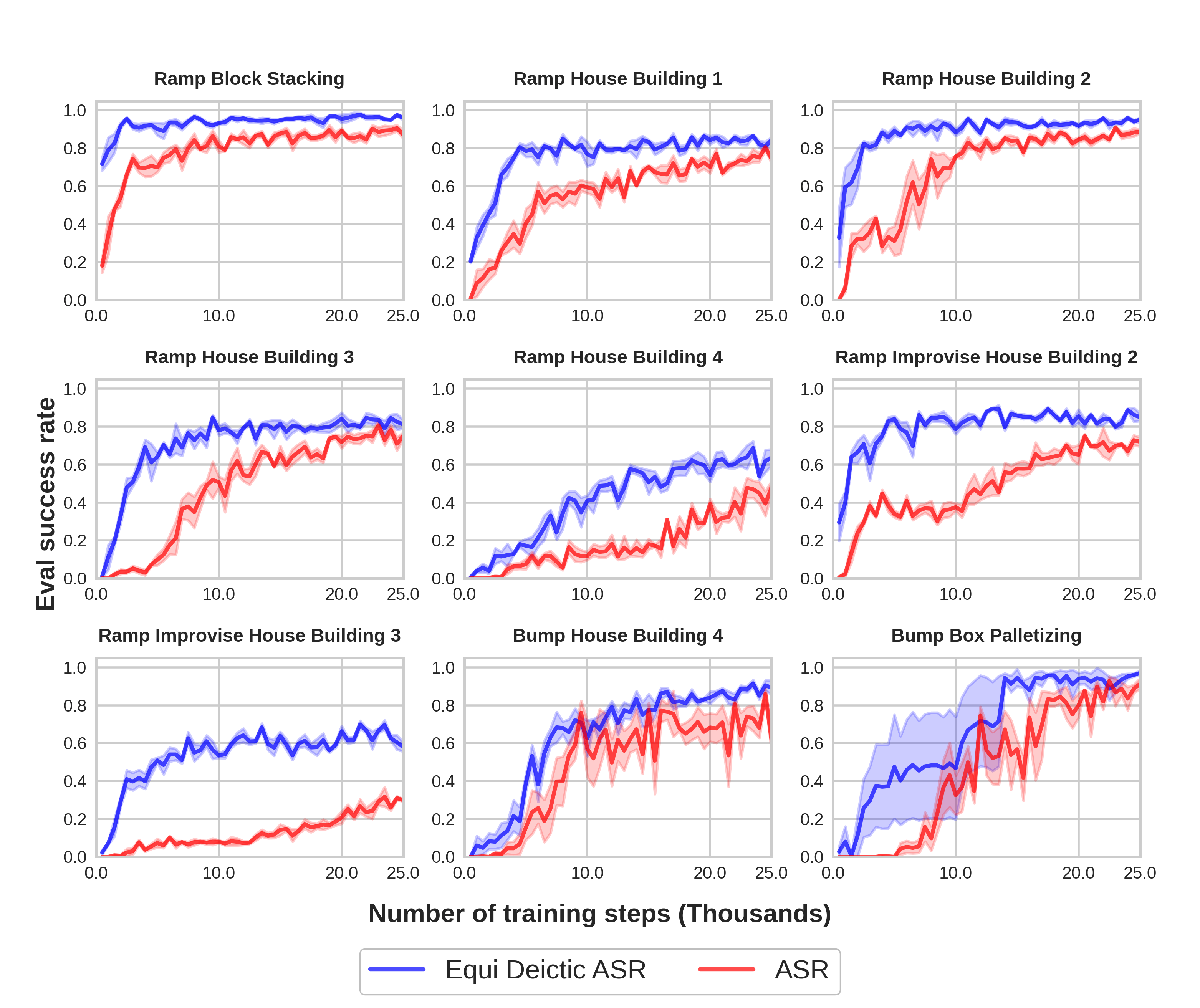
We provide two baselines in this benchmark: 1) ASR [43]: a hierarchical approach that selects the actions in a sequence of using 5 networks; 2) Equivariant Deictic ASR [45] (Equi Deictic ASR): similar as 1), but replace the standard networks with equivariant networks and the deictic encoding to improve the sample efficiency. We use 1000 planner episodes for the ramp environments and 200 planner episodes for the bump environments. The in-hand image in this experiment is a 3-channel orthographic projection image of a voxel grid generated from the point cloud at the previous pick pose. Other environment parameters mirror the Open-Loop 3D Benchmark in Section 5.1.
Figure 19 shows the results. Equivariant Deictic ASR (blue) demonstrates a stronger performance compared with standard ASR (red).
D.3 Close-Loop 3D Benchmark
The Close-Loop 3D Benchmark is similar as the Close-Loop 4D Benchmark (Section 5.2), but with the following two changes: first, the environments are initialized with a fixed orientation; second, the action space is instead of , i.e., the agent only controls the delta position of the end-effector and the open-width of the gripper.
We provide the same baseline algorithms as in Section 5.2. In this section, we show the performance of SDQfD, Equivariant SDQfD (Equi SDQfD), and FERM SDQfD. Figure 20 shows the result. Equivariant SACfD (blue) shows the best performance across all tasks. FERM SACfD (green) and SACfD (red) has similar performance, except for Block Reaching, where FERM SACfD outperforms standard SACfD.
Appendix E Additional Baselines for Open-Loop 3D Benchmark
In this section, we show the performance of three additional baseline algorithms in the Open-Loop 3D Benchmark (Section 5.1): DQfD, ADET, and DQN. We compare them with SDQfD (the algorithm used in Section 5.1). All algorithms are equipped with the Equivariant ASR architecture. Figure 21 shows the result. Notice that SDQfD and DQfD generally perform the best, while SDQfD has a marginal advantage compared with DQfD. ADET learns faster in some tasks (e.g., House Building 1), but normally converges to a lower performance compared with SDQfD and DQfD. DQN performs the worst across all environments because of the lack of imitation loss.
Appendix F Additional Baselines for Close-Loop 4D Benchmark
In this section, we show the performance of two additional baseline algorithms in the Close-Loop 4D Benchmark (Section 5.2): RAD SACfD and DrQ SACfD. As is shown in Figure 22, RAD SACfD (yellow) performs poorly in all 10 environments. DrQ SACfD (brown) outperforms FERM SACfD (purple) in Block Picking and Block Pulling, but still underperforms the equivariant methods (blue and red).
Appendix G Benchmark Details
G.1 Open-Loop Benchmark
In all environments, the kuka arm is used as the manipulator. The workspace has a size of . The top-down observation covers the workspace with a size of pixels. (In the Rot FCN baseline, ’s size is pixels, and is padded with 0 to pixels. This is padding required for the Rot FCN baseline because it needs to rotate the image to encode .) The size of the in-hand image is pixels for the Open-Loop 2D and Open-Loop 3D benchmarks. In the Open-Loop 6D Benchmark, is a 3-channel orthographic projection image, with a shape of in the ramp environments, and in the bump environments. We train our models using PyTorch [32] with the Adam optimizer [22] with a learning rate of and weight decay of . We use Huber loss [16] for the TD loss. The discount factor is . The mini-batch size is . The replay buffer has a size of 100,000 transitions. At each training step, the replay buffer will separately draw half of the samples from the expert data and half of the samples from the online transitions. The weight for the margin loss term of SDQfD is , and the margin . We use the greedy policy as the behavior policy. We use 5 environments running in parallel.
G.2 Close-Loop Benchmark
In all environments, the kuka arm is used as the manipulator. The workspace has a size of . The pixel size of the top-down depth image is (except for the FERM baseline, where ’s size is and will be cropped to ). ’s FOV is . We use the Adam optimizer with a learning rate of . The entropy temperature is initialized at . The target entropy is -5. The discount factor . The batch size is 64. The buffer has a capacity of 100,000 transitions. In baselines using the prioritized replay buffer (PER), PER has a prioritized replay exponent of 0.6 and prioritized importance sampling exponent as in [35]. The expert transitions are given a priority bonus of . The FERM baseline’s contrastive encoder is pretrained for 1.6k steps using the expert data as in [53]. We use 5 environments running in parallel.