Bulk-edge Correspondence in the Adiabatic Heuristic Principle

— Characterization of quantum matter with topological invariants is a modern notion in condensed matter physics Thouless et al. (1982); Kohmoto (1985); Hasan and Kane (2010); Qi and Zhang (2011). The adiabatic deformation of gapped systems is a conceptual basis in the theory of topological phases beyond the Landau’s symmetry breaking paradigm Wen (1989, 2017). Meanwhile, augmented by the symmetry, this notion leads to more unified picture exemplified by the “periodic table” for topologically nontrivial states Kitaev (2009); Schnyder et al. (2008); Qi et al. (2008); Ryu et al. (2010) and demonstrates the existence of rich topological phases. The adiabatic deformation also gives a useful way to characterize concrete models by reducing them to simple systems Greiter and Wilczek (1990, 1992, 2021); Hatsugai (2005, 2006, 2007); Kariyado et al. (2018).

The adiabatic heuristic argument of the quantum Hall (QH) effect Greiter and Wilczek (1990, 1992, 2021) is the historical example in which the adiabatic deformation has been successfully used. The fractional QH (FQH) effect Tsui et al. (1982); Laughlin (1983) is a topological ordered phase Wen (1995) with fractionalized excitations Haldane (1983); Halperin (1984); Arovas et al. (1984). Even though it is intrinsically a many-body problem of correlated electrons unlike the integer QH (IQH) effect Klitzing et al. (1980); Laughlin (1981); Thouless et al. (1982); Halperin (1982), the composite fermion theory Jain (1989, 2007) gives a unified scheme to describe their underlying physics: the FQH state at the filling factor $\nu=p/(2mp\pm 1)$ with $p,m$ integers can be interpreted as the $\nu=p$ IQH state of the composite fermions. By continuously trading the external flux for the statistical one Wilczek (1982a, b), both states are adiabatically connected through intermediate systems of anyons (adiabatic heuristic principle Greiter and Wilczek (1990, 1992, 2021)). Even though the ground state degeneracy Haldane (1985); Wen and Niu (1990) is wildly changed in the periodic geometry Greiter and Wilczek (1992); Kudo and Hatsugai (2020), the energy gap remains open and its many-body Chern number Niu et al. (1985) works well as an adiabatic invariant Kudo and Hatsugai (2020).

Generally bulk topological invariants such as the Chern number are intimately related to the presence of gapless edge excitations. This is the so-called bulk-edge correspondence Wen (1990a); Hatsugai (1993a, b), which is a universal feature of topological phases Kane and Mele (2005); Haldane and Raghu (2008); Hasan and Kane (2010); Qi and Zhang (2011); Kariyado and Hatsugai (2015); Delplace et al. (2017); Sone and Ashida (2019); Hatsugai and Fukui (2016); Kuno and Hatsugai (2020); Mizoguchi et al. (2021); Yoshida et al. (2020). The edges of the QH systems demonstrate the nontrivial transport properties enriched by the bulk topology, which has attracted a great interest for over decades Laughlin (1981); Halperin (1982); MacDonald (1990); Wen (1990b, a, 1991); Johnson and MacDonald (1991); Wen (1992); Chamon and Wen (1994); Wen (1995); Meir (1994); Kane et al. (1994); Kane and Fisher (1995); Wan et al. (2002); Joglekar et al. (2003); Wan et al. (2003); Chang (2003); Hu et al. (2008, 2009); Wang et al. (2013a); Repellin et al. (2018); Fern et al. (2018); Wei et al. (2020); Ito and Shibata (2021); Khanna et al. (2021). The main goal in this work is to reveal how the quantum Hall edge states are evolved during the process of the flux-attachment in the adiabatic heuristic principle.

In this Letter, we analyze the fractional pumping phenomena associated with the Laughlin’s argument of the anyonic FQH effect. We show that the general feature of the energy spectrum with edges shows little change during the process of the flux-attachment while the topological degeneracy is wildly changed. Furthermore, the total jump of the center-of-mass works well as an invariant of this process, which is consistent with the bulk-edge correspondence of the FQH effect of anyons. This implies that the total jump of the center-of-mass characterizes the fractional charge pumping of the adiabatic heuristic principle. Also, this supports the stability of the QH edge states in the adiabatic heuristic principle.

— Let us consider the QH system on a square lattice with $N_{x}\times N_{y}$ sites, where $N_{x}/N_{y}=2$ and the periodic boundary condition is imposed. As shown in Fig. 1(a), local fluxes $\pm\xi$ are set at two plaquettes $A_{\pm}$ with the same $y$ coordinate. Their distance is $N_{x}/2$. Particles are pumped from $A_{-}$ to $A_{+}$ as $\xi$ varies from $0$ to $1$ [see Fig. 1(b)], which we call the (fractional) charge pump Thouless (1983); Wang et al. (2013b); Nakajima et al. (2016); Lohse et al. (2016); Guo et al. (2012); Xu et al. (2013); Zeng et al. (2015); Hu et al. (2016); Zeng et al. (2016); Nakagawa and Furukawa (2017); Taddia et al. (2017); Nakagawa et al. (2018) throughout this Letter.

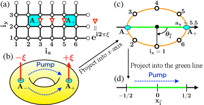
This charge pump can be mapped into the one-dimensional pump with edges [Fig. 1(d)]. As shown in Fig. 1(c), we first project the system into the $x$-axis. Then, projecting it into the green line shown in Figs 1(c), we finally define a new coordinate for site $\vec{i}=(i_{x},i_{y})$ as $x_{\vec{i}}=(1/2)\cos\theta_{\vec{i}}$ with $\theta_{\vec{i}}=2\pi(i_{x}-a_{x})/N_{x}$, where $a_{x}$ is the $x$ coordinate of $A_{+}$, see Fig. 1(d). In this projection, the two pin-holes $A_{\pm}$ are mapped into the edges $x_{\vec{i}}=\pm 1/2$.

The charge can be transformed from $x_{\vec{i}}=-1/2$ to $x_{\vec{i}}=1/2$ as $\xi$ increases. The pumped charge is given by the integration of $\partial_{\xi}P(\xi)$, where $P$ is the center-of-mass,

$\rho$ is the zero temperature density matrix in the grand canonical ensemble and $n_{\vec{i}}$ is the number operator at the site $\vec{i}$. (In Sec. S1 of Supplemental Material sup , we derive the pumped charge by using the current operator.) As $\xi$ varies, $P(\xi)$ jumps several times due to the sudden change of the particle number Hatsugai and Fukui (2016); Kuno and Hatsugai (2020, 2021). Accordingly, the pumped charge between the period $\xi\in[0,1]$ is given by $Q=\left(\int_{0}^{\xi_{1}^{-}}+\int_{\xi_{1}^{+}}^{\xi_{2}^{-}}+\cdots+\int_{\xi_{N}^{+}}^{1}\right)d\xi\,\partial_{\xi}P(\xi)$, where $\xi_{1},\cdots,\xi_{N}$ are the jumping points in the period and $\xi_{\alpha}^{\pm}=\xi_{\alpha}\pm 0$. Using the periodicity $P(1)=P(0)$ and $\Delta P(\xi_{\alpha})\equiv P(\xi_{\alpha}^{+})-P(\xi_{\alpha}^{-})$, we get Hatsugai and Fukui (2016)

As shown below, the total jump $\Delta P_{\text{tot}}$, i.e., the sudden changes of the particle number, comes from the (dis)appearance of edge states. Equation (2) implies that the pumped charge is given only by the information of edges.

— In this Letter, we numerically show the following bulk-edge correspondence for the FQH states of anyons:

where $C$ is the many-body Chern number Niu et al. (1985) of the $N_{D}$-fold degenerate ground state multiplet at $\xi=0$. This is consistent with the Laughlin’s argument applied to the FQH systems Laughlin (1981); Halperin (1982); Thouless et al. (1982); Thouless (1983); Niu et al. (1985); Hatsugai (1993a); Thouless (1989); Hatsugai and Fukui (2016); Zeng et al. (2016); Grushin et al. (2015); Andrews et al. (2021) that implies $Q=C/N_{D}$. In the following, we clarify how the fractional charge pumping is deformed to the standard pumping phenomena by the flux-attachment transformation. As mentioned below, the relation in Eq. (3) results in the stability of the QH edge states in the adiabatic heuristic principle.

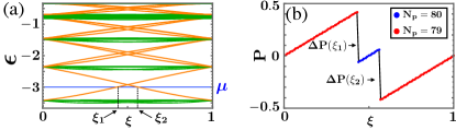
— As a first step, we confirm Eq. (3) for the IQH system of non-interacting fermions. The Hamiltonian is $H=-t\sum_{\langle ij\rangle}e^{i\phi_{ij}}e^{i\xi_{ij}}c_{i}^{\dagger}c_{j}$, where $c_{i}^{\dagger}$ is the creation operator for a fermion on site $i$ and $t=1$. The phase factors $e^{i\phi_{ij}}$ and $e^{i\xi_{ij}}$ describe the uniform magnetic field Hofstadter (1976); Hatsugai et al. (1999) and the local fluxes at $A_{\pm}$ [see Fig. 1(a)], respectively. We plot in Fig. 2(a) the single-particle energy $\epsilon$ with $N_{x}\times N_{y}=40\times 20$ and $\phi\equiv N_{\phi}/(N_{x}N_{y})=1/10$, where $N_{\phi}$ is the total uniform fluxes. Each set of $N_{\phi}(=80)$ states forms the Landau level (LL) at $\xi=0$. As $\xi$ increases, some edge states go over to the mid-gap region. In Fig. 2(b), we compute $P(\xi)$ with $\rho=|{G}\rangle\langle{G}|$ in Eq. (1), where $|{G}\rangle$ is the ground state completely occupying the 1st LL under the chemical potential (Fermi energy) $\mu=-3$. The sudden change of the particle number $N_{p}$ causes the jumps of $P(\xi)$ at $\xi_{1}$ and $\xi_{2}$. Both values of $\Delta P(\xi_{\alpha})$’s are approximately $-1/2$, which is consistent with Fig. 2(a) where one edge state at $x_{\vec{i}}=1/2$ goes over across $\mu$ and then another at $x_{\vec{i}}=-1/2$ goes back. Although a finite size effect gives $\Delta P_{\text{tot}}=\Delta P(\xi_{1})+\Delta P(\xi_{2})\approx-0.96$, we confirm $\Delta P_{\text{tot}}=-1$ in the thermodynamic limit (see Sec. S2 of Supplemental Material sup ). This is consistent with Eq. (3) with $N_{D}=1$ and $C=1$. The cases for $C=2$ and $3$ have been also confirmed.

— As mentioned above, the jump $\Delta P(\xi_{\alpha})$ are not quantized to $\pm 1/2$ due to the finite size effect. Let us then properly normalize each jumps: when $P$ jumps positively or negatively at $\xi_{\alpha}$, we assign it as $\Delta P(\xi_{\alpha})\mapsto 1/2$ or $-1/2$. Hereafter “$\mapsto$” denotes this normalization; e.g., we have $\Delta P_{\text{tot}}=P(\xi_{1})+P(\xi_{2})\mapsto-1/2-1/2=-1$ in Fig. 2(b). This gives the bulk-edge correspondence in Eq. (3) even for finite systems.

—

Let us consider the fractional pumping of anyons. To this end, we take the Hamiltonian as $H=-t\sum_{\langle ij\rangle}e^{i\phi_{ij}}e^{i\xi_{ij}}e^{i\theta_{ij}}c_{i}^{\dagger}c_{j}$, where the phase factor $\theta_{ij}$ Wen et al. (1990); Hatsugai et al. (1991); fer depends on the configuration of all particles $\{\bm{r}_{k}\}_{1\leq k\leq N_{p}}$, which describes the fractional statistics $e^{i\theta}$. Note that although $c_{i}^{\dagger}$ is the creation operator for a fermion, $H$ is the Hamiltonian of anyons and includes intrinsically the many-body interactions. Due to constraints of the braid group, $\dim H$ depends on $\theta$ even for the same $N_{p}$ Wen et al. (1990); Einarsson (1990): the Hilbert space for $\theta/\pi=n/m$ ($n,m$: coprime) is spanned by the basis $|{\{\bm{r}_{k}\};w}\rangle$, where $w=1,\cdots,m$ is an additional internal degree of freedom. When a particle hops across the boundary in the $x$ direction, the label is shifted from $w$ to $w-1$. As for the boundary in the $y$ direction, the phase factor $e^{iw\theta}$ is given. Thanks to this, global requirements of anyons hold GR ; Wen et al. (1990); Einarsson (1990); Hatsugai et al. (1991). Also, we introduce $\xi_{ij}$ only for the basis with $w=1$ def .

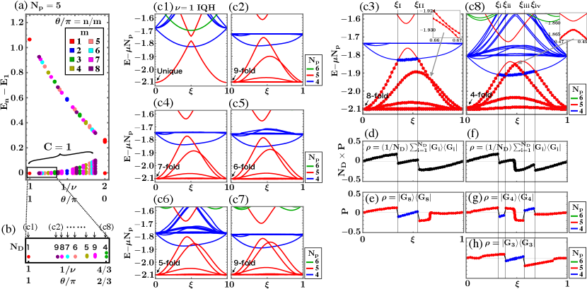
In the following, we focus on a family of the $\nu=1$ IQH states connected by trading the magnetic fluxes for statistical ones Jain (1989); Greiter and Wilczek (1990, 1992); Kudo and Hatsugai (2020): $\nu=p/[p(1-\theta/\pi)+1]$ with $p=1$. Fixing $N_{x}\times N_{y}=10\times 5$, $N_{p}=5$ and $\xi=0$, we plot the energy gaps as functions of $1/\nu$ in Fig. 3(a). Due to the lattice, the topological degeneracy is lifted. We here define the low-energy states with $E_{n}-E_{1}<0.2$ as the ground state multiplet. The ground state at $\nu=s/t$ ($s,t$: coprime) in Fig. 3(a) gives the degeneracy $N_{D}=t$ numerically [see Fig. 3(b)] and the Chern numbers of the multiplets are always $C=1$ Kudo and Hatsugai (2020). Namely, the many-body Chern number is used as an adiabatic invariant. The gap closing at $\nu\approx 1/2$ is expected due to finite-size effects Kudo and Hatsugai (2020).

Let us investigate the pumping phenomena. As for each parameter $(1/\nu,\theta/\pi)$ shown in Fig. 3(b), we plot in Figs. 3(c1)-(c8) the eigenvalues of the Hamiltonian including the chemical potential, $H-\mu N_{p}$, as functions of $\xi$ with $4\leq N_{p}\leq 6$ Np . Figure 3(c1) is in the same setting of Fig. 2 but for smaller system sizes. In Fig 3(c1), the particle number $N_{p}$ of the unique ground state is changed as $\xi$ increases due to the (dis)appearance of the edge state as mentioned previously. The gap between the two red lines at $\xi\approx 0.5$ is a finite-size effect. As shown in Figs. 3(c1)-(c8), even though the topological degeneracy is wildly changed as $1/\nu$ and $\theta/\pi$ vary, the general feature of the spectra remains unchanged. The degenerate ground states at $\xi=0$ are lifted as $\xi$ increases and then one or two states float up in energy to cross with another state having one particle less.

Now we focus on the anyonic system in Fig. 3(c3) and show its the bulk-edge correspondence. Here $\theta/\pi=6/7$, $\nu=7/8$ and $N_{D}=8$ at $\xi=0$. To define the center-of-mass of the ground state multiplet suitably, we define the density matrix as $\rho(\xi)=(1/N_{D})\sum_{k=1}^{N_{D}}|{G_{k}(\xi)}\rangle\langle{G_{k}(\xi)}|$, where $|{G_{k}(\xi)}\rangle$ is the $k$-th lowest energy state. Using it with Eq. (1), we plot $N_{D}\times P(\xi)$ in Fig. 3(d). There are two jumps at $\xi_{\text{I}}$ and $\xi_{\text{II}}$, where the $N_{D}$th and $N_{D}+1$th lowest energy states cross each other in the spectrum. Because of $N_{D}\rho=\sum_{k=1}^{N_{D}}|{G_{k}}\rangle\langle{G_{k}}|$, the obtained jumps are solely given by $P$ with $\rho=|{G_{N_{D}}}\rangle\langle{G_{N_{D}}}|$ shown in Fig. 3(e). This figure gives $\Delta P_{\text{tot}}=\Delta P(\xi_{I})+P(\xi_{II})\mapsto-1$, which implies $N_{D}\times\Delta P_{\text{tot}}\mapsto-1$ in Fig. 3(d). This is consistent with Eq. (3) with $C=1$. Because of $Q=-\Delta P_{\text{tot}}$, we ahve the fractional pumped charge $Q=1/8$. In this argument, we assume the absence of the gap closing between states with the same $N_{p}$ apart from $\xi=0$ since there are no symmetry except for the charge $U(1)$. The gap at $\xi\approx 0.7$ between $|{G_{N_{D}}}\rangle$ and $|{G_{N_{D}-1}}\rangle$ is very small but is finite Two as shown in the inset.

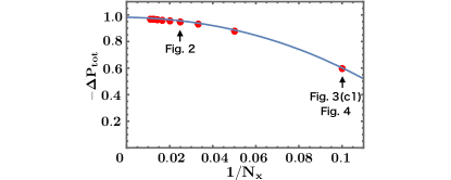
Let us here mention the finite size effect in Fig. 3(d). The value of $N_{D}\times\Delta P_{\text{tot}}$ before normalizing is about $-0.46$, which is far away from $-1$. Although this value in the IQH system in Fig. 3(c1) is about the same magnitude (about $-0.60$, see the data point at $\nu=1$ of Fig. 4), it approaches $-1$ as the system size increases as confirmed in Sec. S2 of Supplemental Material sup . Since the bulk gaps of the two systems are comparable and their system sizes are same, the deviation from $-1$ in Fig. 3(d) is also expected to be the finite size effect.

Let us next focus on the system in Fig. 3(c8), where $\theta/\pi=2/3$, $\nu=3/4$ and $N_{D}=4$ at $\xi=0$. Unlike the previous case, there are four gap-closing points, $\xi_{\text{i}}\cdots\xi_{\text{iv}}$, as for the $N_{D}$ lowest energy states. However, $P(\xi)$ with $\rho=(1/N_{D})\sum_{k=1}^{N_{D}}|{G_{k}}\rangle\langle{G_{k}}|$ in Fig. 3(f) jumps only at $\xi_{\text{i}}$ and $\xi_{\text{iv}}$ because the jumps at $\xi_{\text{ii}},\xi_{\text{iii}}$ cancel each other, see Figs. 3(g) and 3(h). Consequently, the total jump is given by $N_{D}\times\Delta P_{\text{tot}}\mapsto-1$, which is consistent with Eq. (3) with $C=1$. This implies the fractional pumped charge $Q=1/4$. The gap at $\xi\approx 0.5$ is very small but is finite as mentioned before, see the inset in Fig. 3(c8).

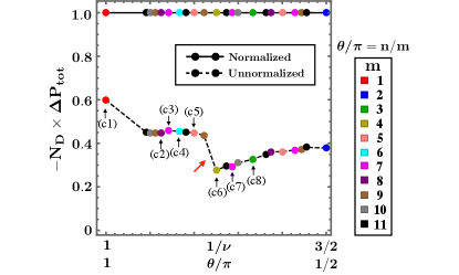
The results shown in Figs. 3(c3) and 3(c8) suggest that $N_{D}\times\Delta P_{\text{tot}}$ is the invariant of the bulk gap in the process of the flux-attachment. To demonstrate it, we plot the total jumps as functions of $1/\nu$ in Fig. 4, where both data before/after normalizing each jumps are shown. The normalized data justify that $N_{D}\times\Delta P_{\text{tot}}$ works well as the invariant. This nature is also indicated by the unnormalized data in Fig. 4: the plots are smooth as $1/\nu$ and $\theta/\pi$ vary even though (i) the degeneracy $N_{D}$ is wildly changed and (ii) the dimension of the Hamiltonian is discretely changed depending on the denominator of $\theta/\pi$: e.g., with $N_{p}=5$, $\dim H=\binom{N_{x}N_{y}}{N_{p}}=\binom{50}{5}=2118760$ for $\theta/\pi=n$ while $\dim H=11\binom{50}{5}=23306360$ for $\theta/\pi=n/11$ (this is due to the additional internal degree $w$ of the basis $|{\{\bm{r}_{k}\};w}\rangle$ as mentioned above). We stress that this nontrivial smoothness in Fig. 4 implies the stability of the QH edge states in the adiabatic heuristic principle.

— In this Letter, we demonstrate the bulk-edge correspondence of the FQH states of anyons. The results indicate that the total jump of the center-of-mass, which corresponds to the many-body Chern number, is an invariant with respect to the flux-attachment. This implies the stability of edge states in the adiabatic heuristic principle. Recently, direct observation of the center of mass in pumping phenomena has been conducted in cold atoms Nakajima et al. (2016); Lohse et al. (2016). The behavior of the center-of-mass that we focus on would be observed in cold atoms although the experimental realization of the two-dimensional anionic system is still a challenging problem.