Budget-constrained rail electrification modeling using symmetric traffic assignment - a North American case study

Rail networks play a vital role in local and national economic structures. In many countries such as Japan and Switzerland, they constitute a significant share of passenger transport mode share. Rail freight transit also accounts for a large portion of total freight transit, exceeding 50% modal share in large economies like Canada and Russia. Therefore, a significant opportunity exists for government policies incentivizing rail network improvements to provide for larger economic, environmental and social returns.

Rail network electrification, and the accompanying transition from diesel-electric to fully electric locomotives, are important steps towards sustainable systems and renewable fuel sources for the United States of America. There are many studies on the impact and cost-benefit analysis of rail electrification [United States Department of Transportation - Federal Railroad Administration (2015), U.S. Department of Transportation - Federal Railroad Administration (2019)]. Advantages of electric locomotion include lower long-term energy and locomotive maintenance costs, lower noise and air pollution levels, faster acceleration, and more flexibility in the primary power source, leading to less volatility from fuel price fluctuations. These benefits must be balanced with significant upfront investment for infrastructure upgrades, higher infrastructure maintenance costs, vulnerability of overhead architecture, higher property tax obligations for private rail companies, and the general uncertainty in the investment [Walthall (2019)].

We consider a rail network design problem (RNDP) where parts of a freight rail network can be electrified, subject primarily to budget constraints. The RNDP is formulated as a bi-level problem: the upper level problem deciding optimal subset of links for electrification, and the lower level problem calculating link flows as well as associated network metrics. Our upper-level formulation uses the objective of minimizing private costs, laying a foundation that can be adapted to improve net social benefit and reflect where subsidies ought to be directed. Given that there are many rail operators, and shippers can choose which operator to use (not necessarily aligning with net social benefit), we model the lower level problem as a user-equilibrium traffic assignment problem (TAP). Genetic algorithms (GA) solve the higher level problem of finding the optimal links to electrify.

In this setting, rather than apportioning an electrification budget to each rail operator independently, a utilitarian schema allocates the electrification budget for specific link electrification in order to bring about the greatest possible cost reductions across the network. The rail operators and shippers then respond to these changes by altering their scheduling and flow patterns to minimize their individual costs. Given multiple operators, the lower level problem is a setting where flow is directed “selfishly,” to minimize shipment costs. For the lower level problem, we assume that these activities lead to an equilibrium, where the costs of shipment flows cannot be lowered unilaterally. With shipment flow expressed in tons, as a continuous quantity over the long term, this problem satisfies the traffic assignment user equilibrium assumptions. Given few self-optimizing fleet owners, we have a Nash-Cournot equilibrium, which in the limit results in user equilibrium flow pattern. \citeNvan1991multiple show that a Nash-Cournot equilibrium for two fleets results in less than 5% difference in avg. travel times (and by extension, total system travel time) for large networks. As the number of fleets increase, this difference decreases and approaches zero. Therefore, we use the user equilibrium assumption in our study. This assumption is consistent with prior literature on the topic  [Uddin and Huynh (2015), Wang et al. (2018)].

Let $\mathbf{A}$ denote the set of rail links traversable by diesel-electric trains, and $\mathbf{N}$ denote the set of nodes (yards and stations). Each link $i\in\mathbf{A}$ currently has a flow-dependent usage cost $c_{i}(x_{i})$ per unit flow. The link can be electrified for a cost of $c^{e}_{i}$, changing the usage cost function to $c^{\prime}_{i}(x_{i})$ per unit flow. The usage costs for diesel and electrified links differ due to technological differences and fuel costs, and are lower for electrified links. The set of candidate links eligible for electrification is denoted by $\mathbf{A^{E}}$, a subset of $\mathbf{A}$. The flow on link $i$ is given by $x_{i}$ tons per day. The capacity of the link is denoted by $u_{i}$. Let $\Pi$ denote the set of paths in the network, and $h_{\pi}$ the flow on a particular path $\pi\in\Pi$.

The set of nodes (denoting stations, yards, interchanges, etc.) is denoted by $\mathbf{N}$. The demand between each origin $r$ and destination $s$ node is given by $d_{rs}$. The demand information between all origin-destination (OD) pairs is stored in the OD matrix $\mathbf{D}$. The total budget for upgrades is $B$. The decision variable $y_{i}$ for $i\in\textbf{A}$ equals 1 if link $i$ is chosen for upgrades (electrification) and 0 otherwise. The cost for switching the mode of operations from diesel to electric (and vice versa) at yard $u$ is $w_{u}$ (and infinitely high at other nodes without switching facilities).

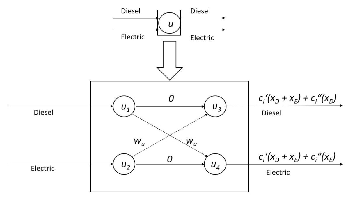
The practical interpretation of link electrification involves additional electric infrastructure on a link allowing electric trains to use the same physical link with different fuel costs, while maintaining the same total link capacity. Our model captures this using the network transformation shown in Figure 1 with a node, an incoming link, and an outgoing link. Each physical link is split into two parallel sub-links, one for diesel flow ($x_{Di}$) and one for electric flow ($x_{Ei}$). The congestion cost $c_{i}^{\prime}$ on each electrified link is not separable, depending on the sum of diesel and electric flows, thus capturing the physical link capacity constraint. The fuel (track resistance) costs $c_{i}^{\prime\prime}$ on these two sub-links are separable, depending only on the sub-links own flow (diesel or electric). The capacity of the electric sub-link is set infinitely high for links not chosen for electrification. Therefore, the total link cost of any link $i$ is $c_{i}(x_{Di}+x_{Ei})=2c_{i}^{\prime}(x_{Di}+x_{Ei})+c_{i}^{\prime\prime}(x_{Di})+c_{i}^{\prime\prime}(x_{Ei})$. Each node $u$ in the network is expanded to incorporate switching costs $w_{u}$. This switching cost is set infinitely high at non-yard nodes to allow switching only at yards.

	$\displaystyle\min\quad\ \$	$\displaystyle\sum_{i\in\mathbf{A}}c_{i}(x_{i})x_{i}$		(1)
	subject	to:
		$\displaystyle\sum_{i\in\mathbf{A}}c^{e}_{i}y_{i}\leq B$		(2)
		$\displaystyle x_{i}=x_{Di}+x_{Ei}\qquad\forall i\in\mathbf{A}$		(3)
		$\displaystyle y_{i}\in\{0,1\}\qquad\forall i\in\mathbf{A}$		(4)

	$\displaystyle\min_{\mathbf{x},\mathbf{h}}\quad\quad$	$\displaystyle\oint_{0}^{\mathbf{x}}\mathbf{c}(\mathbf{s})\cdot d\mathbf{s}$			(5)
	subject to:
	$\displaystyle x_{i}$	$\displaystyle=\sum_{\pi\in\Pi:(r,s)\in\pi}h_{\pi}$	$\displaystyle\forall(r,s)\in\mathbf{A}$		(6)
	$\displaystyle x_{i}$	$\displaystyle\leq My_{i}$	$\displaystyle\forall i\in\mathbf{A^{E}}$		(7)
	$\displaystyle\sum_{\pi\in\Pi^{rs}}h_{\pi}$	$\displaystyle=d_{rs}$	$\displaystyle\forall(r,s)\in\mathbf{N}^{2}$		(8)
	$\displaystyle h_{\pi}$	$\displaystyle\geq 0$	$\displaystyle\forall\pi\in\Pi$		(9)

Equation 1 minimizes the total usage cost over electrified and non-electrified links. Equation 2 enforces the electrification budget constraint. Equation 4 indicates that $y_{i}$ is a binary indicator variable. Equation 5 is the modified Beckmann function for symmetric link interactions, described more in the next sub-section. Equation 6 states that the relation between link and path flows, and Equation 7 ensures that the electrified links with flow are the ones actually chosen for construction. Equation 8 ensures that the demand is met across all used paths for each OD pair, and Equation 9 states flow non-negativity.

We would like to make an important observation here. The total demand is considered constant for our case study, and we conduct preliminary sensitivity analysis to understand the effect of varying (induced) demand. The problem with elastic demand is equivalent to the TAP formulation via the Gartner transformation  [Gartner (1980)] if the model elasticity is fully known. This transformation creates direct links from every origin to destination and captures potential flow increase using the elasticity data on the new links. However, this requires model elasticity to be fully known, and the network size increases by several orders of magnitude. Therefore, despite being equivalent from a method standpoint, we have not incorporated elastic demand in our case study.

This section provides the cost calculation formulae for the link electrification costs, track resistance, and generalized link costs. Owing to a significant number of constants and rates within these formulae, they are omitted here for brevity, but can be found on the author’s github repository [Patil (2020)]. In order to update cost values for inflation, this study uses industry appropriate producer price indices from the \citeNbls.

There are two main costs to be considered, roughly corresponding to the capital expenses and operational expenses. Electrification costs (or capital expenses) refer to all the costs associated with converting a link from standard operations to electric operations that we considered. The generalized link costs (operational expenses) refer to the costs of traversing a link, and incorporate both time and fuel (whether diesel or electricity) costs based on the link’s speed and resistance, calculated on a per-ton basis.

Most algorithms for TAP are designed for the separable cost case. In this sub-section, we describe the changes that need to be made for our cost structure, and derive a new flow shift formula for this case. Our solution method is based on Algorithm B, briefly described in the literature review. The main points of this algorithm are disaggregating link flows by origin, where the sets of used links form acyclic subnetworks; shifting flows from longer-cost segments to shortest-cost segments within each subnetwork; and updating these subnetworks by removing unnecessary links and adding new ones which provide shorter paths.

Of these three components, the original derivation of only the second component (flow shift) relies on separable link costs, and must be re-examined in light of interactions. We first show that link interactions in our formulation satisfy the symmetry condition needed for the formulation (5)–(9) to hold, and then re-derive the flow shift formula for Algorithm B with interactions.

As discussed in the Cost Formulae section, all flow continuing on the same fuel type has zero switching cost, whereas all flow changing fuel type has pre-defined switching costs. Note that only the parallel diesel-electric link pair has cost function dependent on the sum of the flows (see Figure 1), and $c^{\prime}(x)$ is identical for both links. The Jacobian takes the form:

$$J_{\mathbf{x}}=\begin{pmatrix}\frac{\partial(c_{1}(\mathbf{x}))}{\partial x_{1}}&\frac{\partial(c_{2}(\mathbf{x}))}{\partial x_{1}}&\cdots&\frac{\partial(c_{n}(\mathbf{x}))}{\partial x_{1}}\\ \frac{\partial(c_{1}(\mathbf{x}))}{\partial x_{2}}&\frac{\partial(c_{2}(\mathbf{x}))}{\partial x_{2}}&\cdots&\frac{\partial(c_{n}(\mathbf{x}))}{\partial x_{2}}\\ \vdots&\vdots&\ddots&\vdots\\ \frac{\partial(c_{1}(\mathbf{x}))}{\partial x_{n}}&\frac{\partial(c_{2}(\mathbf{x}))}{\partial x_{n}}&\cdots&\frac{\partial(c_{n}(\mathbf{x}))}{\partial x_{n}}\\ \end{pmatrix}$$

The off-diagonal elements are zero whenever the two links do not interact. In our case, the only non-zero off diagonal elements are for parallel diesel-electric pairs. These elements are calculated using the chain rule:

$$\frac{\partial c^{\prime}(x_{D}+x_{E})+c"(x_{D})}{\partial x_{E}}=\frac{\partial c^{\prime}(x_{D}+x_{E})}{\partial(x_{D}+x_{E})}.\frac{\partial(x_{D}+x_{E})}{\partial x_{E}}=\frac{\partial c^{\prime}(x_{D}+x_{E})}{\partial(x_{D}+x_{E})}$$

(16)

$$\frac{\partial c^{\prime}(x_{D}+x_{E})+c"(x_{E})}{\partial x_{D}}=\frac{\partial c^{\prime}(x_{D}+x_{E})}{\partial(x_{D}+x_{E})}.\frac{\partial(x_{D}+x_{E})}{\partial x_{D}}=\frac{\partial c^{\prime}(x_{D}+x_{E})}{\partial(x_{D}+x_{E})}$$

(17)

As can be seen, these two derivatives are identical, proving that the Jacobian is a symmetric matrix, and establishing the validity of the formulation (5)–(9).

We next show that the Algorithm B flow shift procedure (equalizing cost between routes) is valid even in the presence of link interactions. This result is more general, and can be applied to any instance of symmetric costs depending on at most two links, not just the ones we adopt in our study. We separate out the terms involving interactions as follows: $c_{i}=f_{1}(x_{i},x_{j})+f_{2}(x_{i})$ and $c_{j}=g_{1}(x_{i},x_{j})+g_{2}(x_{j})$, with $\frac{\partial f_{1}(x_{i},x_{j})}{\partial x_{j}}=\frac{\partial g_{1}(x_{i},x_{j})}{\partial x_{i}}$. For our rail electrification formulation, $f_{1}(x_{i},x_{j})=g_{1}(x_{i},x_{j})=c_{i}^{\prime}(x_{D},x_{E})$, resulting in a simpler problem.

In this flow-shift operation, we have identified two paths (a lower-cost path $\pi_{L}$ and a higher-cost $\pi_{U}$), and wish to shift flow between them to minimize the objective. Recall that the line integral formulation can now be written as:

$$F(\mathbf{x})=\oint_{\mathbf{0}}^{\mathbf{x}}\mathbf{c}(\mathbf{s})\cdot d\mathbf{s}$$

(18)

Partition the arc set $\mathbf{A}$ into three subsets $A_{1}$, $A_{2}$, and $A_{3}$. Links in set $A_{3}$ have separable cost, depending only on their own flow. The travel time on the links in sets $A_{1}$ and $A_{2}$ depend on the flows on two links: the link itself, and exactly one link in the other set. Mathematically, there is a bijection between sets $A_{1}$ and $A_{2}$, with the notation $i(j)$ and $j(i)$ used to denote the counterparts of links in the other set. The notation for these cost functions lists the links own flow first, and its counterpart’s flow second, that is, $c_{i}(x_{i},x_{j(i)})$ and $c_{j}(x_{j},x_{i(j)})$. Let $p=|A_{1}|=|A_{2}|$ and $m=|A_{1}|+|A_{2}|+|A_{3}|$. The index $a$ will be used to denote a generic link, if it doesn’t matter which set it’s from.

As the line integral is path-independent, we choose the following integration path:

$$(0,0,0,\ldots,0)\rightarrow(x_{1},0,0,\ldots,0)\rightarrow(x_{1},x_{2},0,\ldots,0)\rightarrow\cdots\rightarrow(x_{1},x_{2},\ldots,x_{m})\,.$$

The line integral then decomposes into a sum of ordinary integrals:

	$\displaystyle F(\mathbf{x})=$	$\displaystyle\sum_{i=1}^{p}\int_{(x_{1},\ldots,x_{i-1},0,0,\ldots,0)}^{(x_{1},\ldots,x_{i-1},x_{i},0,\ldots,0)}c_{i}(\mathbf{s})\cdot d\mathbf{s}+\sum_{j=p+1}^{2p}\int_{(x_{1},\ldots,x_{j-1},0,0,\ldots,0)}^{(x_{1},\ldots,x_{j-1},x_{j},0,\ldots,0)}c_{j}(\mathbf{s})\cdot d\mathbf{s}$
		$\displaystyle+\sum_{k=2p+1}^{m}\int_{(x_{1},\ldots,x_{k-1},0,0,\ldots,0)}^{(x_{1},\ldots,x_{k-1},x_{k},0,\ldots,0)}c_{k}(\mathbf{s})\cdot d\mathbf{s}$
	$\displaystyle=$	$\displaystyle\sum_{i=1}^{p}\int_{0}^{x_{i}}c_{i}(s,0)~{}ds+\sum_{j=p+1}^{2p}\int_{0}^{x_{j}}c_{j}(s,x_{i(j)})~{}ds+\sum_{k=2p+1}^{m}\int_{0}^{x_{k}}c_{k}(s)~{}ds\,.$

Let $I_{a}$ be $+1$ if link $a$ is on $\pi_{L}$, $-1$ if $a$ is on $\pi_{U}$, and $0$ otherwise. Then for a flow shift $\Delta x$ from the longest to the shortest path, the change on each link’s flow is given by $\Delta x_{a}=I_{a}\Delta x$ and $I_{a}=\partial(\Delta x_{a})/\partial(\Delta x)$. (This latter equation will be used when differentiating via the chain rule below). The objective in terms of a flow shift of size $\Delta x$ is now

$$F(\Delta x)=\sum_{i=1}^{p}\int_{0}^{x_{i}+\Delta x_{i}}c_{i}(s,0)~{}ds+\sum_{j=p+1}^{2p}\int_{0}^{x_{j}+\Delta x_{j}}c_{j}(s,x_{i(j)}+\Delta x_{i(j)})~{}ds+\sum_{k=2p+1}^{m}\int_{0}^{x_{k}}c_{k}(s)~{}ds\,,$$

and when we differentiate with respect to $\Delta x$, we obtain the following (the second term splits into two terms from the Leibniz rule):

$$\frac{dF}{d(\Delta x)}=\sum_{i=1}^{p}c_{i}(x_{i}+\Delta x_{i},0)I_{i}+\sum_{j=p+1}^{2p}c_{j}(x_{j}+\Delta x_{j},x_{i(j)}+\Delta x_{i(j)})I_{j}\\ +\sum_{j=p+1}^{2p}\int_{0}^{x_{j}+\Delta x_{j}}\frac{\partial c_{j}}{\partial x_{i(j)}}(s,x_{i(j)}+\Delta x_{i(j)})I_{i(j)}~{}ds+\sum_{k=2p+1}^{m}c_{k}(x_{k}+\Delta x_{k})I_{k}\,.$$

We will show that $dF/d(\Delta x)=\sum_{a\in(\mathbf{A}\cup\mathbf{A^{E}})}c_{a}(\mathbf{x}+\Delta\mathbf{x})I_{a}$. The interpretation is that the derivative vanishes if $\Delta x$ equalizes the cost difference on the longest and shortest segments, thus minimizing the Beckmann function. The second and fourth terms in the sum are exactly what we need for the links in $A_{2}$ and $A_{3}$. We need to show

$$\sum_{i=1}^{p}c_{i}(x_{i}+\Delta x_{i},0)I_{i}+\sum_{j=p+1}^{2p}\int_{0}^{x_{j}+\Delta x_{j}}\frac{\partial c_{j}}{\partial x_{i(j)}}(s,x_{i(j)}+\Delta x_{i(j)})I_{i(j)}~{}ds\\ =\sum_{i=1}^{p}c_{i}(x_{i}+\Delta x_{i},x_{j(i)}+\Delta x_{j(i)})I_{i}\,.$$

Using the symmetry condition $\frac{\partial c_{j}}{\partial x_{i(j)}}=\frac{\partial c_{i}}{\partial x_{j(i)}}$, we have

$\displaystyle\sum_{i=1}^{p}c_{i}(x_{i}+\Delta x_{i},0)I_{i}+\sum_{j=p+1}^{2p}\int_{0}^{x_{j}+\Delta x_{j}}\frac{\partial c_{i}}{\partial x_{j(i)}}(s,x_{i(j)}+\Delta x_{i(j)})I_{i(j)}~{}ds\,.$

Using the fundamental theorem of calculus and one-to-one correspondence of terms in the two summations, it is clear that it equals $\sum_{i=1}^{p}c_{i}(x_{i}+\Delta x_{i},x_{j(i)}+\Delta x_{j(i)})I_{i}$, which is the required form. Therefore, $dF/d(\Delta x)=\sum_{a}c_{a}(\mathbf{x}+\Delta\mathbf{x})I_{a}$ and Algorithm B flow shifts are valid in our setting. Most implementations of Algorithm B (including ours) use a Newton method to equalize the costs on these links. The denominator in Newton’s method (the flow shift scaling factor) can also be adjusted to reflect interactions[Patil and Boyles (2022)], but even without this change, existing implementations still converge to the equilibrium.

After obtaining solutions and validating the solution method for our formulation, the second set of experiments involves policy testing and sensitivity analysis. These experiments vary parameters such as total budget, demand data, electrification costs, electricity costs, crew/cargo costs, policy changes in the form of monetary incentives. The base electrification budget is $30 billion, roughly equivalent to electrifying $65,000$ kilometers of track. This is varied by up to $\pm 20\%$, or $24–36 billion. The analysis involves studying the return on investment (ROI) in the form of reduced costs, incentivizing policymakers and private stakeholders to upgrade infrastructure.

Freight Analysis Framework, version 4 (FAF4) provides demand data from 2010 and 2020, as well as forecasts for 2030 and 2040 [Bureau of Transportation Statistics (2020)]. In addition, lowering the usage cost of rail freight allows for modal shift from trucking to rail. This potential demand variation is considered by increasing the demand data by up to 25% from base values. Lastly, electrification costs and crew/cargo costs are also tested at increased values (+25%) to gauge effects on the electrification solution. Note that under the current experiment formulation, adjusting the electrification costs is equivalent to adjusting the budget for electrification.

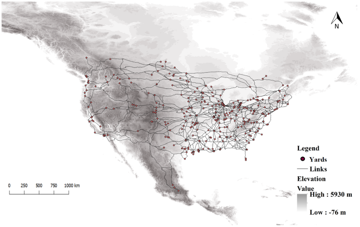
The North American railroad network has been extracted from the statewide analysis module [Alliance Transportation Group (2013)] provided by the Texas Department of Transportation, originally based on the CTA rail network developed at Oak Ridge National Laboratory [Center for Transportation Analysis (2014)]. The dataset includes 35,424 links, and has geographical information (length, latitude, longitude, grade category), ownership information, and other auxiliary information. There are 28,289 nodes connected by these links, denoting stations, yards and interchanges. Elevation data were obtained by overlaying the network on the North American elevation grid [U.S. Geological Survey (2007)] using ArcGIS (Figure 2(a)). The demand data (in tons) has been obtained from FAF4 [Bureau of Transportation Statistics (2020)]. We would like to note that directional running (like implemented by Union Pacific in Texas) can result in increased flow efficiency, and can be modeled using increased link density. Barring detailed information on directional running, we have not included it in our model.

As specified, operational mode changes can only occur at yards. Therefore, corridor electrification is more sensible than individual link electrification. Candidate corridors were obtained by connecting each yard to the nearest neighboring yards. Specifically, the following method was employed to find the set of candidate corridors and results can be seen in Figure 2(b). This new shortest corridor network has tracks totaling $170,000$ kms of track available for electrification, down from over $305,000$ kms in the full network. The switching costs were obtained using the following assumptions for the locomotives: 1.5 hours to switch, throttle position 1 for diesel-electrics, 10% power for electrics, and 6 crew-equivalents manpower.

1. 1.

   Calculate all pair shortest paths (APSP) from all yards

2. 2.

   Calculate APSP from all yards, but prune search branch after reaching a yard.

3. 3.

   Compare the two sets and keep the paths common to both sets

All result visualizations are shown in Figures 3–6. The low budget, base case (medium budget), and high budget cases lead to electrification of about 49,000 (30,000), 61,000 (36,000), and 70,500 (42,000) kms (mi), respectively. Only the base case results are shown with the full network backdrop, all other results are shown on the shortest path corridor network for better visibility. Figures 4 - 6 show the results as the overlap of different scenarios. Figure 4 is a cumulative plot, where the medium budget (base case) and high budget results are shown as increments over the low budget case. Figures 5 and 6 pivot off the base case, therefore, we highlight the overlapping links as well as the differences.

The first observation is that the GA retained all corridors selected for the low budget case in the base case and high budget case. However, this changes for the increased demand and increased costs scenarios, given that the network OD matrix and costs change in the two scenarios. This allows us to identify the most impactful corridors and stations, such as all three of the major transcontinental routes (LA-Chicago, Oakland-Chicago, and Seattle-Chicago), which the algorithm chooses for electrification in each scenario. There is a wide variety of corridors selected across the entire network. The algorithm selects quite a few mountainous routes where electrification provides the most benefits per train, but the algorithm also appears to select for links that provide connectivity throughout the network. This trend is best illustrated in figure 6, which seems to show that the increased demand case shifts the selection from the more mountainous west to the more populous east and gulf coasts. With higher demand, links that provide smaller benefits per train are more likely to provide greater benefits overall.

Examining the base case in further detail, the algorithm selects 13.2% of the network (by line-miles) for electrification, and predicts that 15.5% of final flow (by tonnage) will use electrical traction. This reflects that busier corridors benefit more from electrification. This also implies that most of the traffic along electrified links would be using electric rather diesel-electric locomotives.

The increased demand scenario increases electrified corridor connectivity to several new yards/stations. The increased cost scenario reduces selection from east and central US, and chooses corridors from western US. We hypothesize this selection occurs due to the higher elevations and grades for these tracks seeing benefit from electrification. The current formulation does not incorporate any regional variations in the wholesale cost of electricity or diesel.

Each sub-problem took 5 minutes to converge, and each GA instance took  36 hours to finish on a Linux PC with i7 Processor (2.6 GHz) and 16 GB RAM. Given the long-term planning horizon, runtimes are not crucial, but still useful to scalability of the heuristic for a large network.

This study presents a novel way of looking at the rail network electrification problem using connections to the road traffic assignment problem. We formulate the problem as a bi-level network design problem, where the lower level problem is a symmetric traffic assignment problem, assigning goods flow instead of traffic. We then show the correctness of Algorithm B flow shift formula for the symmetric traffic assignment problem, using it to solve this sub-problem. The costs and network parameters incorporate electrification costs; fuel, locomotive, and operational costs; and train resistance costs.

The North American railroad network is used as a test network to demonstrate our method, show scalability for large networks, and draw insights. We observe and note some corridors chosen in all different testing scenarios (varying budgets, opex, and demand), as well as provide policy insights for planning. The key observations are as follows:

• •

  While there seems to be some evidence of corridors in more mountainous terrain producing better cost savings, overall there is a wide variety of corridors selected across the entire network. This implies that providing broad connectivity might be more important than electrifying the corridors with the best savings on a per-train basis.

• •

  The results for the increased demand case, shown in figure 5, indicate a shift in chosen corridors from the more mountainous west towards the more populous east and gulf coasts. This is probably a result of the increased demand causing those corridors to generate higher savings, even though they have fewer savings per train. This is also evidence that the highest priority corridors might be routes through rough terrain operating at or near capacity.

• •

  Sensitivity to demand means long-term trends in the trucking industry could have a substantial influence on the highest priority corridors for electrification.

The main limitations of this work are: 1) static power levels (once calculated); 2) static brake usage assumption on links; 3) static electricity and diesel costs; and 4) lack of incorporation of track ownership restrictions on path selection. The first three limitations are relatively straightforward to tackle, although they increase problem complexity and computation time significantly by introducing another layer of iterative calculations.

An additional complication is partly based on the data available: because this analysis uses large zones with few centroids, the simulations might overestimate the benefit of electrifying well-traveled corridors that connect multiple zones. Studying how the selection changes based on varying switching costs might show whether the results are skewed by simulating a higher amount of connectivity than would actually exist. This problem could partially be ameliorated by applying a cost to electric trains reaching centroid connectors to reflect that some electric trains might require additional drayage over diesel-electric trains. Properly calibrating such a cost would remain a difficult problem.

The methods formulated in this study can be adapted to consider social benefits from changes in emissions, formulating the problem as one of social benefit maximization rather than private cost minimization. The composition of the power grid affects the emissions an electric locomotive causes, meaning the marginal social benefits of electrification and the marginal private cost savings can vary substantially from link to link. In some parts of the power grid where most of the electricity is provided by coal, an electric train might even produce more emissions than an equivalent diesel-electric train [Walthall (2019)]. Understanding social benefits is important because the high variability of private return-on-investment from electrification might necessitate public subsidies before capital construction becomes possible. Prior studies have formulated social benefit maximization problems as a single-level problems, thus reducing computational complexity.

All data, models, and code generated or used during the study appear in the submitted article.

The authors would like to thank William Alexander and Karthik Velayutham for their insights and help with the TAP code implementation. This research was partially supported by the National Science Foundation (CMMI-1562291, CMMI-1826320).

References

- Alliance Transportation Group (2013) Alliance Transportation Group (2013). “Statewide Analysis Model - Third Version (SAM-V3).
- Bar-Gera (2010) Bar-Gera, H. (2010). “Traffic assignment by paired alternative segments.” Transportation Research Part B: Methodological, 44(8-9), 1022–1046.
- Beckmann et al. (1956) Beckmann, M., McGuire, C. B., and Winsten, C. B. (1956). “Studies in the economics of transportation.” Report No. RM-1488-PR, RAND corporation.
- Borndörfer et al. (2008) Borndörfer, R., Grötschel, M., and Pfetsch, M. E. (2008). “Models for line planning in public transport.” Computer-aided systems in public transport, Springer, 363–378.
- Boyles et al. (2020a) Boyles, S., Alexander, W., Patel, R., Velayutham, K., and Thakkar, R. (2020a). “tap-b implementation.” https://github.com/spartalab/tap-b/wrap Accessed: 2020-05-20.
- Boyles et al. (2020b) Boyles, S. D., Lownes, N. E., and Unnikrishnan, A. (2020b). Transportation Network Analysis, Vol. 1. 0.85 edition.
- Bureau of Public Roads (1964) Bureau of Public Roads (1964). Traffic Assignment Manual for Application with a Large, High Speed Computer, Vol. 37. US Department of Commerce, Bureau of Public Roads, Office of Planning.
- Bureau of Transportation Statistics (2020) Bureau of Transportation Statistics (2020). “Freight analysis framework version 4.” https://faf.ornl.gov/fafweb/ Accessed: 2020-07-25.
- Cambridge Systematics (2012) Cambridge Systematics (2012). “Task 8.3: Analysis of freight rail electrification in the scag region.” http://www.freightworks.org/DocumentLibrary/CRGMSAIS%20-%20Analysis%20of%20Freight%20Rail%20Electrification%20in%20the%20SCAG%20Region.pdf Accessed: 2020-07-27.
- Center for Transportation Analysis (2014) Center for Transportation Analysis (2014). “CTA Railroad Network Accessed: 2018-10-03.
- Chen and Alfa (1991) Chen, M. and Alfa, A. S. (1991). “A network design algorithm using a stochastic incremental traffic assignment approach.” Transportation Science, 25(3), 215–224.
- Clarke (1995) Clarke, D. B. (1995). “An examination of railroad capacity and its implications for rail-highway intermodal transportation.” Ph.D. thesis, University of Tennessee - Knoxville,
- Dafermos (1971) Dafermos, S. C. (1971). “An extended traffic assignment model with applications to two-way traffic.” Transportation Science, 5(4), 366–389.
- Dafermos (1972) Dafermos, S. C. (1972). “The traffic assignment problem for multiclass-user transportation networks.” Transportation science, 6(1), 73–87.
- Dial (2006) Dial, R. B. (2006). “A path-based user-equilibrium traffic assignment algorithm that obviates path storage and enumeration.” Transportation Research Part B: Methodological, 40(10), 917–936.
- Ditmeyer et al. (1985) Ditmeyer, S., Martin, J., Olson, P., Rister, M., Ross, B., Schmidt, J., and Sjokvist, E. (1985). “Railway electrification and railway productivity: A study report.” Transportation Research Record, 1029.
- Drezner and Wesolowsky (1997) Drezner, Z. and Wesolowsky, G. O. (1997). “Selecting an optimum configuration of one-way and two-way routes.” Transportation Science, 31(4), 386–394.
- Farahani et al. (2013) Farahani, R. Z., Miandoabchi, E., Szeto, W. Y., and Rashidi, H. (2013). “A review of urban transportation network design problems.” European Journal of Operational Research, 229(2).
- Fritz, S.G. (2000) Fritz, S.G. (2000). “Diesel fuel effects on locomotive exhaust emissions.” Report No. 08.02062, Southwest Research Institute, San Antonio, TX.
- Gao et al. (2005) Gao, Z., Wu, J., and Sun, H. (2005). “Solution algorithm for the bi-level discrete network design problem.” Transportation Research Part B: Methodological, 39(6), 479–495.
- Gartner (1980) Gartner, N. H. (1980). “Optimal traffic assignment with elastic demands: a review part ii. algorithmic approaches.” Transportation Science, 14(2), 192–208.
- Gattuso and Restuccia (2014) Gattuso, D. and Restuccia, A. (2014). “A tool for railway transport cost evaluation.” Procedia-Social and Behavioral Sciences, 111, 549–558.
- Gillespie and Hayes (2003) Gillespie, A. J. and Hayes, H. I. (2003). “Practical guide to railway engineering.” AREMA committee-24, USA.
- Hay (1982) Hay, W. W. (1982). Railroad engineering, Vol. 1. John Wiley & Sons.
- Iliopoulou et al. (2019) Iliopoulou, C., Kepaptsoglou, K., and Vlahogianni, E. (2019). “Metaheuristics for the transit route network design problem: a review and comparative analysis.” Public Transport, 11(3), 487–521.
- Jayakrishnan et al. (1994) Jayakrishnan, R., Tsai, W. T., Prashker, J. N., and Rajadhyaksha, S. (1994). “A faster path-based algorithm for traffic assignment.
- Katoch et al. (2021) Katoch, S., Chauhan, S. S., and Kumar, V. (2021). “A review on genetic algorithm: past, present, and future.” Multimedia Tools and Applications, 80(5), 8091–8126.
- Kneschke (1986) Kneschke, T. (1986). “Simple method for determination of substation spacing for ac and dc electrification systems.” IEEE Transactions on Industry Applications, IA-22(4).
- Lawrence et al. (2019) Lawrence, M., Bullock, R., and Ziming, L. (2019). “China’s High-Speed Rail Development Accessed: 2021-10-20.
- Leblanc (1975) Leblanc, L. J. (1975). “An algorithm for the discrete network design problem.” Transportation Science, 9(3), 183–199.
- Lo and Szeto (2004) Lo, H. K. and Szeto, W. (2004). “Planning transport network improvements over time.” Urban and regional transportation modeling: Essays in honor of David Boyce, 157–176.
- Lo and Szeto (2009) Lo, H. K. and Szeto, W. (2009). “Time-dependent transport network design under cost-recovery.” Transportation Research Part B: Methodological, 43(1), 142–158.
- Long et al. (2010) Long, J., Gao, Z., Zhang, H., and Szeto, W. Y. (2010). “A turning restriction design problem in urban road networks.” European Journal of Operational Research, 206(3), 569–578.
- Meng et al. (2001) Meng, Q., Yang, H., and Bell, M. G. (2001). “An equivalent continuously differentiable model and a locally convergent algorithm for the continuous network design problem.” Transportation Research Part B: Methodological, 35(1), 83–105.
- Ministry of Railways (India) (2020) Ministry of Railways (India) (2020). “Railway Electrification Accessed: 2021-10-20.
- Mishra et al. (2016) Mishra, S., Kumar, A., Golias, M. M., Welch, T., Taghizad, H., and Haque, K. (2016). “Transportation investment decision making for medium to large transportation networks.” Transportation in Developing Economies.
- Nektalova (2008) Nektalova, T. (2008). “Energy Density of Diesel Fuel Accessed: 2020-07-30.
- Patil (2020) Patil, P. (2020). “Rail electrification data repository.” https://github.com/PriyadarshanPatil/Rail_electrification_GA Accessed: 2020-07-25.
- Patil and Boyles (2022) Patil, P. N. and Boyles, S. D. (2022). “A fresh look at symmetric traffic assignment and algorithm convergence.” Proc., 101th Annual Meeting, Transportation Research Board. Accepted.
- Patriksson (1994) Patriksson, M. (1994). The traffic assignment problem: models and methods. VSP.
- Perederieieva et al. (2015) Perederieieva, O., Ehrgott, M., Raith, A., and Wang, J. Y. (2015). “A framework for and empirical study of algorithms for traffic assignment.” Computers & Operations Research, 54, 90–107.
- Prager (1954) Prager, W. (1954). Problems of traffic and transportation.
- RailTEC (2016) RailTEC (2016). “Transitioning to a zero or near-zero emission line-haul freight rail system in california: Operational and economic considerations.” https://ww3.arb.ca.gov/railyard/docs/uoi_rpt_06222016.pdf Accessed: 2020-07-27.
- Schwarm (1977) Schwarm, E. G. (1977). “Capital and maintenance costs for fixed railroad electrification facilities.” Transportation Research Board Special Report, 180.
- Szeto et al. (2010) Szeto, W. Y., Jaber, X., and O’Mahony, M. (2010). “Time-dependent discrete network design frameworks considering land use.” Computer-Aided Civil and Infrastructure Engineering, 25(6).
- Szeto and Lo (2006) Szeto, W. Y. and Lo, H. K. (2006). “Transportation network improvement and tolling strategies: the issue of intergeneration equity.” Transportation Research Part A: Policy and Practice, 40(3), 227–243.
- Szeto and Lo (2008) Szeto, W. Y. and Lo, H. K. (2008). “Time-dependent transport network improvement and tolling strategies.” Transportation Research Part A: Policy and Practice, 42(2), 376–391.
- Uddin and Huynh (2015) Uddin, M. M. and Huynh, N. (2015). “Freight traffic assignment methodology for large-scale road–rail intermodal networks.” Transportation Research Record, 2477(1), 50–57.
- United States Department of Transportation - Federal Railroad Administration (2015) United States Department of Transportation - Federal Railroad Administration (2015). “Cost-benefit analysis of rail electrification for next generation freight and passenger rail transportation.” https://cms8.fra.dot.gov/sites/fra.dot.gov/files/fra_net/19061/Cost%20Benefit%20Analysis%20of%20Rail%20Electrification.pdf.
- U.S. Bureau of Labor Statistics (2020) U.S. Bureau of Labor Statistics (2020). “Producer price indexes.” https://www.bls.gov/ppi.
- U.S. Department of Transportation - Federal Railroad Administration (2019) U.S. Department of Transportation - Federal Railroad Administration (2019). “Federal-state partnership for state of good repair grant program (fy 2019).” https://railroads.dot.gov/grants-loans/competitive-discretionary-grant-programs/federal-state-partnership-state-good-repair-0 Accessed: 2020-05-25.
- U.S. Geological Survey (2007) U.S. Geological Survey (2007). “North america elevation 1-kilometer resolution grid.” https://www.sciencebase.gov/catalog/item/4fb5495ee4b04cb937751d6d.
- Van Vuren and Watling (1991) Van Vuren, T. and Watling, D. (1991). “A multiple user class assignment model for route guidance.” Transportation research record, 22–22.
- Walthall (2019) Walthall, R. (2019). “Rail electrification’s potential for emissions abatement in the freight industry : a case study of a transcontinental rail corridor.” M.S. thesis, The University of Texas at Austin, , https://hdl.handle.net/2152/80502.
- Wang et al. (2018) Wang, H., Nozick, L., Xu, N., and Gearhart, J. (2018). “Modeling ocean, rail, and truck transportation flows to support policy analysis.” Maritime Economics & Logistics, 20(3), 327–357.
- Wardrop and Whitehead (1952) Wardrop, J. G. and Whitehead, J. I. (1952). “Correspondence. some theoretical aspects of road traffic research..” Proceedings of the Institution of Civil Engineers, 1(5), 767–768.
- Whitford (1981) Whitford, R. K. (1981). Railroad Electrification: An Alternative for Petroleum Saving. Automotive Transportation Center, Purdue University.