Brightest Cluster Galaxies and Intra-Cluster Light: Their Mass Distribution in the Innermost Regions of Groups and Clusters
Abstract
We improve the model presented in Contini & Gu (2020) that describes the radial mass distribution of brightest cluster galaxies (BCGs) and the diffuse component also known as intra-cluster light (ICL), by assuming that the global BCG+ICL radial mass distribution follows the sum of three profiles: a Jaffe and an exponential profiles for the bulge and disk of the BCG, respectively, and a modified version of an NFW profile for the ICL. We take advantage of a wide sample of BCG+ICL systems simulated with our state-of-art semi-analytic model to: (a) investigate the reliability of our BCG+ICL distribution by looking at several scaling relations between the BCG+ICL stellar mass within different apertures and the total BCG+ICL/halo mass, at different redshift; (b) make a prediction of the distance where the radial distribution transitions from BCG to ICL dominated. We find that our model nicely reproduces all the observed scaling relations investigated at the present time with a compelling degree of precision, but slightly biased-low with respect to observations at higher redshifts (). The transition radius predicted by our model is in good agreement with recent observational results, and spans a range between kpc and kpc. It mostly depends on the morphology of the BCG, whether it is bulge or disk dominated, on the amount of ICL with respect to the bulge and/or disk, and on the dynamical state of the group/cluster.
1 Introduction
Discovered for the first time by Zwicky (1937), the Intra-Cluster Light (hereafter ICL) is a diffuse light in groups and clusters from stars that are not gravitationally bound to any galaxy, and which can extend to several hundreds kpc (Gonzalez et al. 2005; Zibetti et al. 2005; Krick & Bernstein 2007; Gonzalez et al. 2013; Giallongo et al. 2014; Zhang et al. 2019; Henden et al. 2020 and references therein). In the recent past, many attempts, both theoretical and observational (Puchwein et al. 2010; Rudick et al. 2011; Presotto et al. 2014; Contini et al. 2014; Burke et al. 2015; DeMaio et al. 2015; Edwards et al. 2016; Tang et al. 2018; Montes & Trujillo 2019; Kluge et al. 2020; Contini & Gu 2020; Spavone et al. 2020; Furnell et al. 2021, and references therein), have been made in order to study the formation and evolution of this peculiar component, and to highlight its importance in the context of the growth of galaxy clusters and their dynamical state.
Most of the above quoted studies (and many others) agree on the fact that the ICL forms mainly via tidal stripping of intermediate/massive galaxies and mergers of galaxies orbiting around the potential well of the cluster (see Contini et al. 2018, 2019 and references therein for a detailed discussion, or Mihos et al. 2017; Montes 2019 for reviews). From the theoretical point of view, it is almost trivial111For the sake of truth it is not very straightforward to distinguish between merger and stripping channels in the very moment two galaxies are starting to merge simply because there is not a clear definition of when a merger starts. This isssue is particularly important in simulations. to isolate the contribution of each channel of the formation of the ICL. Observationally speaking, it is possible to look at properties of the ICL such as metallicity and color and compare them with the typical metallicity or color of galaxies (e.g., DeMaio et al. 2015; Morishita et al. 2017; Iodice et al. 2017; Montes & Trujillo 2018; Iodice et al. 2020) to understand what channel contributes the most.
Regardless of the processes that bring to the formation of the ICL, or the main contributors to it, in the very last years a few authors (e.g., Montes & Trujillo 2019; Kluge et al. 2020; Alonso Asensio et al. 2020; Contini & Gu 2020; Deason et al. 2021; Poliakov et al. 2021) have focused on the link between the ICL and the dark matter distributions, to figure out whether or not the ICL can be used as a tracer of the dark matter in clusters. By using a sample of six clusters from the Hubble Frontier Fields (Lotz et al. 2017), Montes & Trujillo (2019) compared the bi-dimensional distribution of the dark matter with that of the ICL making use of the Modified Hausdorff distance (MHD), which gives the idea of how far two distributions are from each other. They found that the average distance between the ICL and the dark matter within 140 kpc from the center is around 25 kpc, which is a very short distance considering the size of typical galaxy clusters. Kluge et al. (2020) investigated on the ICL-cluster alignment with a sample of around 50 local clusters and focused on the ICL-cluster and brightest cluster galaxy (hereafter BCG)-cluster alignments. They found that the ICL is better aligned than the BCG with the host cluster in terms of both position and centering. These results strongly suggest that the ICL follows the global dark matter distribution and can be used as a tracer of it. Similarly, Alonso Asensio et al. (2020) used the Cluster-EAGLE simulations (Barnes et al. 2017; Bahé et al. 2017) to test the results mentioned above. By using the same procedure used in Montes et al., they found that the stellar mass distribution follows that of the total, including dark matter, but their radial profiles differ substantially.
In our last paper (Contini & Gu 2020, hereafter CG20), we developed an ICL profile to study its distribution in galaxy groups and clusters for a sample of more than 300 BCGs, whose properties were obtained by means of our semi-analytic model. We started from the idea, supported by the recent observational results mentioned above, that the ICL can follow the dark matter distribution. Hence, we assumed that the ICL follows an NFW (Navarro et al. 1997) profile and added a new parameter, that we called , which is linked to the halo concentration by the relation . The parameter has been then set to reproduce the observed relation, between the BCG-ICL stellar mass in the innermost 100 kpc and the halo mass. By testing our model against several observational and theoretical results, we found that is required to match the observed at , while larger values of are needed at higher redshift, with also hints for a possible halo mass dependence. We then concluded that an NFW like profile is a good description of the ICL distribution in groups and clusters, making the ICL a reliable tracer of the dark matter.
The idea of adopting an NFW profile to describe the distribution of the ICL is not original. For example, Zibetti et al. (2005) found that the observed ICL profile can be approximated by an NFW. They analysed the spatial distribution and color of the ICL taking advantage of a sample counting almost 700 galaxy clusters between and selected from the first release of the Sloan Digital Sky Survey (SDSS-DR1, Abazajian et al. 2003), finding that the radial distribution of the ICL is more centrally concentrated than that of the galaxies, a result which well agrees with our assumption. Recently, some evindence come from the study of Zhang et al. (2019). These authors use around 300 galaxy clusters between and selected from the Dark Energy Survey (DES, McClintock et al. 2019) and focus on the detection of the ICL. Among various interesting results, they find that the ICL radial profile is self-similar and scales with the virial radius of the clusters and that the ICL brightness is a good tracer of the cluster radial mass distribution, in agreement with the studies quoted above. There is evidence also from the theoretical side. Just to mention one, Pillepich et al. (2018) studied the properties of the ICL as predicted by the IllustrisTNG hydrodynamical simulation and found that the radial distribution of the ICL is as shallow as that of the dark matter, meaning that the ICL can effectively trace the overall cluster mass distribution.
The aim of this paper is to further improve the model developed in CG20, where BCGs and ICL have been treated as separated components when we focused on the relation, but BCGs have been assumed to be entirely contained within 100 kpc, a fair assumption in many cases. Here, we treat a BCG as a two-component system, bulge and disk, and model each of them in order to get their mass within any given distance from the center. This approach allows us to enter the very innermost regions of the clusters where BCGs are placed, and compare our model predictions with a variety of observed relations. The ICL is still assumed to follow a modified NFW profile as in CG20, and we focus mainly at the present time given the fact that, in CG20, we found the best match between our predictions and observed relation at . Once we show that our improved model matches a plethora of observed results, we use it to investigate the differential mass distribution as a function of clustercentric distance of the three component, bulge, disk and ICL, for different case studies. We will show that, despite common assumptions frequently used, the ICL can be the dominant component even at very low distances from the cluster centre.
The paper is organized as follows. In Section 2 we briefly describe our semi-analytic model and the profile used to describe any single component. In Section 3 we present our analysis, which will be fully discussed in Section 4. In Section 5 we sum up our main conclusions. Throughout this paper we use a standard cosmology, namely: , , , , and . Stellar masses are computed with the assumption of a Chabrier (2003) Initial Mass Function (IMF), and all units are corrected.
2 Methods
We make use of the semi-analytic model developed in Contini et al. (2014), and further improved in Contini et al. (2018, 2019), which contains a full description of the formation and evolution of the ICL. For a detailed description of the mechanisms that bring to the formation of the ICL, we refer the reader to the papers quoted above, while below we give a short summary of the main features of the semi-analytic model (hereafter SAM) in the context of this work.
As most of nowadays SAMs, ours runs on the merger trees of N-body simulations. Mergers trees contain all the information about the formation and growth of dark matter haloes and subhaloes and constitute the input of our SAM, which, according to the initial conditions (cosmological parameters) of the numerical simulations, places galaxies in haloes and follow them along time by considering the most important physical mechanisms in galaxy formation, i.e. gas cooling, star formation, SN and AGN feedback, mergers and stellar stripping.
In this work we use the merger trees extracted from the same set of high-resolution simulations used in CG20, whose details can be found in Contini et al. (2012). Our sample accounts for 361 groups and clusters at with a virial mass () that spans over two orders of magnitude, from and up to more than .
As in CG20, we model the formation of the ICL by making use of the model ”Tidal Radius” described in Contini et al. (2014) and further improved in Contini et al. (2018). The prescription is applied to satellite galaxies orbiting around central galaxies. The SAM derives a tidal radius for each satellite galaxy, which is assumed to be a two-component system, bulge and disk. If is contained within the bulge, the satellite is assumed to be completely disrupted, while if is larger than the bulge but smaller than the size of the disk, the mass in the shell between and the radius of the disk is stripped. In both cases, all the stripped stellar mass is added to the ICL component associated with the BCG. Another prescription, which considers the stellar mass of satellites stripped during mergers, is implemented and accounts for the so-called merger channel. At each merger, a percentage of 20% of the stellar mass of the satellite is added to the ICL component that is associated with the BCG, and the rest of the mass ends up to the BCG stellar mass.
The details of the other minor assumptions concerning the description of the mechanisms that brings to the formation of the ICL can be found in the papers quoted above. Below, we describe how we model the mass distribution of BCGs, bulge and disk, and the mass distribution of the ICL.
2.1 Bulge and Disk Profiles
We assume a BCG to be a two-component system: bulge and disk. The bulge is assumed to follow a Jaffe profile (Jaffe 1983):
| (1) |
where is the total mass of the bulge and the scale length. By integrating, the mass contained within a sphere of radius is given by
| (2) |
For the disk, we assume an exponential profile and its mass within a given radius is given by:
| (3) |
where is the total stellar mass in the disk, and the scale radius of the disk. By splitting the BCG in the two components, we are able to drop the assumption made in CG20, that is the stellar mass of the BCG is entirely contained in the innermost 100 kpc. With this approach, we can probe distances much below 100 kpc.
2.2 ICL Profile
We model the mass profile of the ICL exactly as in CG20, by assuming a modified version of the NFW profile. The reason behind our choice is fully discussed in CG20 and in Section 1 of this paper. The NFW profile reads as follows:
| (4) |
where is the characteristic density of the halo at the time of its collapse and is its scale radius. The concentration of a dark matter halo is defined as
| (5) |
where is the virial radius of the halo. The modification we made in CG20 to the classic NFW profile described in Equation 4 is by introducing a free parameter in Equation 5. We define the ICL concentration as
| (6) |
In CG20 we argued that the parameter could be a function of halo properties such as the halo mass, and redshift. We set by matching the observed at different redshifts (not considering any halo dependence) and we found that at and higher values at higher redshifts, which means that the ICL is more concentrated than the dark matter halo in which it is contained. As mentioned in CG20, this is in good agreement with recent theoretical works (e.g. Contini et al. 2018; Pillepich et al. 2018) and observational studies (e.g. Montes & Trujillo 2019).
3 Results
In this section we test our model of BCG-ICL in the innermost regions of clusters, below 100 kpc, by looking at the relation between (where is a given distance from the centre) and the halo/BCG mass, and their fraction with respect to the total (Section 3.1). We show that our model compares well with observational results, and we use the success of our model in reproducing those observed quantities to investigate the mass distribution of each component as a function of distance from the cluster centre for a few case studies (Section 3.2).

3.1 Model-Observation Comparisons
In Figure 1 we show the predicted relation, i.e. the BCG-ICL stellar mass between 10-100 kpc and the halo mass at different redshifts (different panels), compared with the observed relation by DeMaio et al. (2020) at similar redshift. As explained above, the values of used are at and at higher redshifts. This figure is similar to Figure 2 in CG20, with the exception that the first 10 kpc are not considered. As in CG20, we find a reasonable agreement with the observed relations, in particular at the present time. Nevertheless, it appears clear that our model tends to underpredict, although for dex, the observed relation at . The degree of the agreement at , instead, is definitely excellent as it is in Figure 2 of CG20 where we account for also the first 10 kpc.

In order to investigate whether our model overpredicts the amount of stellar mass in the first 10 kpc, in Figure 2 we plot the ratio between the stellar mass within 10 kpc and that within 100 kpc, as a function of the halo mass and at different redshifts (different panels). Once again, our predictions (color lines) are compared with the observed data by De Maio et al. (black symbols). The agreement looks better than that found in Figure 1, at least at , although it is clear that our predictions are somewhat higher than the observed data. Considering the fact that the predicted mass within 100 kpc is either similar or lower than observed, it suggests that our model predicts a slightly higher amount of stellar mass in the first 10 kpc. Moreover, regardless of the redshift, less massive haloes have higher than more massive ones. This results from the fact that the parameter is fixed with halo mass, but less massive haloes are intrinsecally more concentrated than more massive ones. Hence, on average, the percentage of ICL within the first 10 kpc is higher for less massive haloes.

To give more credit to our model, we now investigate on the BCG-ICL mass within different apertures, and on their ratio over the total, as a function of halo and BCG mass. Since observations are so far better reproduced by our model at , we will focus only at the present time. In Figure 3 we plot the BCG-ICL mass within 30, 50 and 70 kpc as a function of halo mass, as predicted by the model (black lines), and as observed (red symbols) by Kravtsov et al. (2018). Our model can predict the right amount of BCG-ICL mass within different apertures for a wide range of halo mass. Similarly, Figure 4 shows the same information, but as a function the BCG-ICL mass. In order to be consistent with the set of observed data, we derived the amount of BCG-ICL mass within a given radius that is a function of halo mass (see Kravtsov et al. 2018 for further details). Once again, our model is in very good agreement with the observed data.


In Figure 5 we plot the ratio between the BCG-ICL within the same apertures and the total BCG-ICL mass within as a function of halo mass (a similar plot can be obtained as a function of the BCG-ICL mass with similar information). Our model predictions (black lines) compare well with the observed data (red symbols) for a wider range of halo mass with respect to the similar plots in Figure 2. Overall, the model is able to capture the trend shown by the observed data, and as already seen in Figure 2, with less massive haloes having a larger concentration of mass in the innermost regions than more massive haloes. In this case, being the normalization higher, the trend is even more visible. However, contrary to Figure 2, here the model seems to be somewhat biased low rather than high. We will come back on this in Section 4.
3.2 The Internal BCG-ICL Mass Distribution
As shown in the previous subsection, our model is able to predict several observed scaling relations between the BCG-ICL mass within different apertures and halo/BCG-ICL total mass, in particular at . We now make use of our model to probe the mass distributions as a function of distance from the cluster centre of the three main components (bulge, disk and ICL) separately, that is the main purpose of this study.


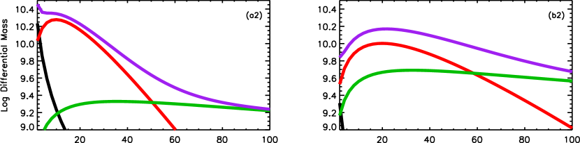

The first four panels of Figure 6 show the diffferential stellar mass of bulge (black line), disk (red line), ICL (green line) and their sum (purple line) as a function of clustercentric distance for four BCG-ICL systems with different mass, ranging from (panel a1), to . These case studies have been chosen almost randomly from our sample, with the only condition of being in the lowest quartile of the mass range (a1), some percentiles before and after the median (b1 and c1), and in the highest quartile (d1). No other condition regarding the mass in the bulge or disk has been chosen, neither about the morpholgy of the BCGs, or halo mass. For these “random” case studies, it is quite evident that the total BCG+ICL stellar mass does not give a real indication of which component (and from where) starts to dominate the total distribution. This is more clear in the last four panels (a2, b2, c2 and d2) of the same figure, which are a zoom-in of the previous four of the innermost regions. In all cases the bulge, as expected, drops very fast, while disk and ICL dominate the total distributions at different clustercentric distances, with the only exception given by d2 for which the mass in the disk is small compared to that in the bulge. Very interestingly, the ICL starts to dominate the total distribution at very small radii, even at 15-20 kpc.
We now move the attention to other four case studies: two pairs of BCG-ICL systems with similar mass and disk/ICL mass ratio. Their differential mass for each component as a function of distance is shown in Figure 8, four a pair with and disk/ICL mass (panels a1 and b1), and a pair with and disk/ICL mass (panels c1 and d1). Again, the four BCGs have been chosen in a random manner among those in our sample, with the only conditions of having same total mass and disk/ICL mass ratio for members of each pair, and similar total mass but different disk/ICL mass ratio for pair-pair members. For these case studies, the picture looks quite different with respect to the previous ones. Indeed, all case studies have a discreet disk/ICL mass ratio, that translates in a more relevant importance of the disk compared to the ICL. From panel a1 to d1 (similar mass but increasing disk/ICL mass ratio) we can see that the disk is increasingly important, and this makes the ICL dominate the total distribution at larger radii than seen before. This trend is more visible in the zoom-in shown in the last four panels of the same figure. As expected, the bulge drops even faster because these are BCGs with a prominent disk, and the importance of the disk with respect to the ICL makes all the difference. In the two cases where the disk is a quarter of the ICL (a2 and b2), the latter starts to dominate at radii kpc, but when the disk is half of the ICL, the distribution of the latter meets the total one at farther distances, kpc in the case c2 and kpc in case d2.
It appears clear that in disk-like BCGs the ICL is less likely to dominate from the innermost regions, while for bulge-like BCGs, given the fact that the bulge drops faster than the disk, it is more likely. We address this point in Figure 10, where we show other two pairs of case studies with similar mass and bulge/BCG mass ratio and plot again the differential mass of each component as a function of distance. The first two cases (a1 and b1) are two disk-like BCGs with B/T and , and the second two cases (c1 and d1) are two bulge-like BCGs with B/T and . For these four cases the conditions were medium size disky BCGs and two bulge-like BCGs on the last quartile of the mass range. The reasons behind our choices is that we want to see the difference bewteen BCGs of different morphology and, at the same time, whether or not in a bulge-like BCG the ICL can dominate the total distribution in a similar way as in a smaller disky BCG. In the first two cases the disk is the component that ”competes” with the ICL and the bulge does not contribute much, while in the last two cases the bulge makes the difference and an almost absent disk does not contribute. The main features of these plots can be seen in the zoom-in provided in the last four panels of the same figure. Similar to previous cases where the disk is important with respect to the ICL, the latter component starts to dominate the total distribution at large distances (over 100 kpc), but the interesting aspect is that in massive bulge-like BCGs the ICL can be important only at distances beyond 60-70 kpc.
With all the previous case studies of different BCG-ICL systems we have shown that the ICL can be the most important component, and so not neglected, even at very small clustercentric distances such as 10-20 kpc. Moreover, the morpholgy of the BCGs, the importance of the mass in the disk with respect to that of the ICL as well as the relative importance of the total BCG mass with respect to that of the bulge, are parameters that weigh on the distance at which the ICL begins to be the only component at play, and the range of distances can be as wide as kpc. In the next section we will further discuss all our results, but mainly those of the second part of our analysis in light of the common assumptions that are generally made when distinguishing between BCG and ICL.
4 Discussion
One of the most serious problems in studying the ICL come directly from its own definition (e.g., Rudick et al. 2011; Cui et al. 2014; Jiménez-Teja & Dupke 2016; Montes & Trujillo 2018; Zhang et al. 2019). Indeed, different authors use different definitions and this happens in both theoretical and observational sides, which makes comparisons among different studies quite complicated. Measuring the ICL is already a hard task, and attempts to separate it from the BCG complicate the job even more, simply because the two components are overlapped in the region dominated by the BCG and the transition between them is supposed to be smooth. Theoretical speaking, it is quite easy to define the ICL because in both semi-analytics and hydrosimulations it is possible to take advantage of information not allowed to observers (see, for example, Rudick et al. 2011 for a detailed review of the most common methods).
On the other hand, in observations, the picture is rather different. Among the years, mainly two are the methods that have been constantly used in observational studies. The easiest way is to apply some cut in surface brightness after removing all the contribution from other sources, such as satellite galaxies and sky. All the light fainter than the cut is defined as ICL, and the rest is given by the BCG (e.g Burke et al. 2015; Montes & Trujillo 2018; Spavone et al. 2020; Iodice et al. 2020 and references therein). As mentioned above, clearly this method might severely underestimate the contribution of the ICL in the innermost regions where it overlaps with the BCG, and thus, might overestimate that of the BCG. This approach is similar, methodologically speaking, to assume a given distance from the center where the light profile drops and follows a plateau, and assume that from there on the ICL is the only component. The other common approach is to use functional forms as we have done in CG20 (and in this paper), that allows to distribute the light of BCGs and ICL (e.g., Kravtsov et al. 2018; Zhang et al. 2019; Kluge et al. 2020; Montes et al. 2021). To quote a few them, Montes et al. (2021) use GALFIT (Peng et al. 2002) to fit a double (one for the BCG and one for the ICL) Sersic (Sersic 1968) profile. Similarly to Kravtsov et al. (2018), Zhang et al. (2019) used a combination of three Sersic profiles: one for the inner core, one for the bulge and one for the ICL. Either with a double or triple Sersic profile, the different components dominate a different distance from the centre. We will come back on this point below.
4.1 Is Our Model Reliable?
In Section 3.1 we presented the analysis done in order to set our model, by comparing our predictions with observational data by DeMaio et al. (2020) up to redshift , and by Kravtsov et al. (2018) at the present time. Overall we find a compelling agreement with observations, but a key point it is worth discussing deeper. When we plot the relation at different redshifts, we find a gap of about dex between our predictions and the observed ones at redshift . A similar gap has been found in CG20 when we included the innermost 10 kpc. The question that rises naturally is: Is this gap real or explainable by invoking intrisic differences between the model and the observation? For real we mean that, as a matter of fact, it implies an evolution in mass since redshift of a factor that it is not seen in the observed data. In CG20 we have addressed this point. As a possible cause for the gap we have argued that, while our predictions are exactly at that particular redshifts, and present time, the observational data by DeMaio et al. span a wider range of redshift with median at . Another possible reason is that our BCG+ICL mass are actually lower than observed at that redshift, which could be due to the difficulty in dectecting the stellar mass at higher redshift given by all the masking done for separating the source from the sky. It might also be that our model, at least in part, underestimates the BCG+ICL mass at .
According to DeMaio et al., it is possible to reconcile the theoretical prediction of our model (since it predicts a rapid evolution of the ICL at late times, Contini et al. 2014) with their data if most of the ICL growth actually occurs at kpc, which is a very reasonable explanation. However, here we try to investigate the innermost tens kpc by assuming a mass profile for every component of a BCG+ICL system, and a direct comparison with their data shows that, although minor, our model does show some evolution within 100 kpc from to the present time. The current state of affairs does not allow us to answer to the question above, because the gap is small for making final statements. Nevertheless, while we suggest the need to have more data at in order to get a more complete picture and a fairer comparison, we surely stress that the profiles we assumed might not completely describe the internal BCG+ICL mass distribution at any redshift, even though they do at the present time.
DeMaio et al. correctly explain that the BCG+ICL gains stellar mass in the range 10-100 kpc more rapidly than within 10 kpc by invoking the “inside-out” scenario (van Dokkum et al. 2010; Patel et al. 2013; Bai et al. 2014; van der Burg et al. 2015; Zhang et al. 2016, 2019 and others) for the growth of the stellar mass distribution. Despite the issue discussed above, our model agrees well with this scenario. Indeed, albeit our predictions are slightly biased low with respect to the observed data, the trend is reproduced, i.e., as a cluster grows in halo mass, it gains more stellar mass from the outer regions (see Figure 2).
We then conclude that our model is reliable at least at the present time, while it needs more testing at higher redshift when more data are available. Hence, a model with a Jaffe profile for the bulge, an exponential one for the disk, and an NFW distribution of the ICL mass can be a good description of the whole BCG+ICL system. In the light of this, we now discuss the main point of this paper, that is, at what distance from the centre the ICL starts to dominate the mass distribution.
4.2 Where Does the ICL Dominate the Mass Distribution?
In Section 3.2 we have investigated the mass distribution of several case studies of BCG+ICL systems by looking at the distribution of each component. We have shown that the distance from which the ICL starts to dominate the total distribution strongly depends on the BCG properties, such as its morphology and whether or not it has an extended disk. The radius at which the ICL dominates the total distribution (for the sake of simplicity let’s call it hereafter) can be very short, around 10-20 kpc, but it might reach even over 100 kpc, depending on the particular case. The total BCG+ICL stellar mass does not seem to play an important role (Figure 6), while the relative contribution of the disk with respect to the ICL (Figure 8) and that of the bulge with respect to the total BCG mass (Figure 10) do.
The morphology, bulge/disk-like BCG, has a major role in determining from where the ICL becomes the dominant component. It is plausible and somewhat expected that BCG+ICL systems where the BCG has an extended disk had larger , and bulge-like BCGs, depending on the mass of their bulge, more or less shorter . Having or not an extendend disk depends mostly on the merger history of the particular BCG, mainly whether or not it has experienced a recent major merger, which totally destroys the disk. However, the disk can further form again if there is enough cold gas and time. Mergers, on the other hand, contribute also on the production of the ICL, i.e., the more the number of mergers experienced, the more the mass that will end up in the ICL component. We can distinguish among three different case scenarios that might explain the BCG+ICL distribution for BCGs (a) bulge dominated (the most common), (b) spheroidals with similar bulge and disk components, and (c) disk-like BCGs (rare objects).
In the case (a), such BCGs either have had a troubled merger history ceasing the star formation before a new disk could grow again (a1), or they had a very recent major merger and no time available to grow a new disk (a2). In the case (a1) the amount of ICL is expected to be large, given the fact that mergers do contribute to the ICL and it is very likely that stellar stripping would play an important role when satellite galaxies are merging. In the case (a2), most depends whether the ICL formed through stellar stripping at late times. Case (b) represents a sort of middle ground between (a) and (c). These BCGs might have had mergers in the past (and so formed ICL), but no recent major merger so that the disk could grow again. For disk-like BCGs, i.e. case (c), it is very likely that they did not have any major merger in the recent past (or at all), and they evolved mainly through smooth accretion/minor mergers and via star formation until gas has been available. However, such BCGs are very rare and constitute a class of BCGs for which their ICL should not be expected to be the relevant component.
Given these three possible scenarios for the formation and evolution of BCG+ICL systems, spans a wide range. It is the shortest for systems where the BCG is a bulge-like galaxy in the low end of the mass rank, and the highest where the BCG has a prominent disk. Overall, considering our case studies, we find that 15 kpc kpc, but can be even larger than 100 kpc in very particular cases. Let’s discuss our results in the context of the most recent observational evidence.
Recently, Montes et al. (2021) focused on a deep study of the ICL of the Abell 85 galaxy cluster by using archival data taken with Hyper Suprime-Cam on the Subaru Telescope. They measured the BCG+ICL surface brightness profile out to around 215 kpc in the g and i bands, and noticed that, at kpc, both the surface brightness and color profiles become shallower. The interpretation of this result is that the ICL starts to dominate at that radius. Not only, in agreement with the prediction of our model (Contini et al. 2014, 2019) the color profile at radius beyond 100 kpc is consistent with that of massive satellite galaxies, suggesting that the stripping of these objects is responsible for the build-up of the ICL. Their kpc is also in good agreement with kpc by Zibetti et al. (2005), who found a similar flattening of the profile at that radius. It must be noted that the value of by Zibetti et al. is the result of a stacking of about 700 galaxy clusters taken by the SDSS. This value of the transition radius at which the ICL becomes the dominant component agrees fairly well with works (e.g., Gonzalez et al. 2005; Seigar et al. 2007; Iodice et al. 2016; Gonzalez et al. 2021) that showed that BCG+ICL systems have such a break in the profile in the range 60-80 kpc.
Similar numbers have been found by Zhang et al. (2019) from the analysis of about 300 galaxy clusters at redshift . These authors described the BCG+ICL radial profile by using a triple Sersic model and found a dominant core in the innermost 10 kpc, a bulge between 30 and 100 kpc and the ICL that dominates the distribution beyond 200 kpc, but already outside 100 kpc the profile transitions from the BCG to the ICL. They suggested that this transition is a potential cut between the two components, in good agreement with Pillepich et al. 2018 who noticed that simulated haloes more massive than have more ICL mass outside 100 kpc than within.
All the values of the transition radius, i.e. the radius at which the ICL starts to become the dominant component, reported above are comparable with the range predicted by our model. We stress again that, a wide range of possible values of is preferable to a narrow one for the reasons discussed above. It strongly depends on the morphology of the BCG, of the amount of ICL with respect to the other components and, not as last, to the dymanical state of clusters, which reflects the merging history of the BCG+ICL system and so its evolution with time.
5 Conclusions
Following the analysis done in our recent paper (Contini & Gu 2020), we have further improved our model by assuming that the radial mass distribution of a BCG+ICL system can be described by the sum of three profiles: a Jaffe profile for the bulge, an exponential disk and a modified NFW for the ICL. We have taken advantage of a wide sample of simulated galaxy groups and clusters from our state-of-art semi-analytic model to study the innermost kpc of BCG+ICL systems. Unlike the model used in our previous study, the new one offers the opportunity to go below 100 kpc since bulge and disk are treated separately. The main goals of this study were to confirm that our model can reproduce several observed relations between the stellar mass at a given radius and the total BCG+ICL/halo mass, at different redshift and, give an idea of where the transition between the BCG and the ICL happens, i.e. when the ICL component starts to dominate the total distribution. In the light of the analysis done and the overall discussion, we conclude the following:
-
•
the radial mass distribution of a BCG+ICL system can be described by the sum of three profile: a Jaffe profile for the bulge, an exponential disk and a NFW-like profile for the ICL. The model can reproduce several observed scaling relation between the BCG+ICL stellar mass within a given aperture and the BCG+ICL/halo mass, at different redshift with an overall precision below 0.05 dex at and 0.3 dex at along the wide stellar mass/halo mass ranges probed.
-
•
In good agreement with recent observational studies, our model predicts that , i.e. the radius at which the radial distribution of BCG+ICL systems, transitions from the BCG to the ICL, ranges from kpc to kpc. The transition radius, however, depends on BCG properties such as its morphology, bulge/disk-like galaxy, on the amount of ICL with respect to the other components, and to the dymanical state of the group/cluster.
In a future study we aim to better set the model at higher redshifts by investigating the parameter , that links the concentration of the ICL to that of the halo, and its relation between halo mass and redshift. In order to do that, we need more observational data at where our model seems to show some bias with respect to the data used in this study.
Acknowledgements
The authors thank the anonymous referee for his/her constructive comments which helped to improve the manuscript. This work is supported by the National Key Research and Development Program of China (No. 2017YFA0402703), and by the National Natural Science Foundation of China (Key Project No. 11733002).
References
- Abazajian et al. (2003) Abazajian, K., Adelman-McCarthy, J. K., Agüeros, M. A., et al. 2003, AJ, 126, 2081. doi:10.1086/378165
- Alonso Asensio et al. (2020) Alonso Asensio, I., Dalla Vecchia, C., Bahé, Y. M., et al. 2020, MNRAS, 494, 1859
- Bahé et al. (2017) Bahé, Y. M., Barnes, D. J., Dalla Vecchia, C., et al. 2017, MNRAS, 470, 4186
- Bai et al. (2014) Bai, L., Yee, H. K. C., Yan, R., et al. 2014, ApJ, 789, 134. doi:10.1088/0004-637X/789/2/134
- Barnes et al. (2017) Barnes, D. J., Kay, S. T., Bahé, Y. M., et al. 2017, MNRAS, 471, 1088
- Burke et al. (2015) Burke, C., Hilton, M., & Collins, C. 2015, MNRAS, 449, 2353
- Chabrier (2003) Chabrier, G. 2003, PASP, 115, 763
- Contini et al. (2012) Contini, E., De Lucia, G., & Borgani, S. 2012, MNRAS, 420, 2978
- Contini et al. (2014) Contini, E., De Lucia, G., Villalobos, Á., & Borgani, S. 2014, MNRAS, 437, 3787
- Contini et al. (2018) Contini, E., Yi, S. K., & Kang, X. 2018, MNRAS, 479, 932
- Contini et al. (2019) Contini, E., Yi, S. K., & Kang, X. 2019, ApJ, 871, 24
- Contini & Gu (2020) Contini, E. & Gu, Q. 2020, ApJ, 901, 128. doi:10.3847/1538-4357/abb1aa
- Cui et al. (2014) Cui, W., Murante, G., Monaco, P., et al. 2014, MNRAS, 437, 816. doi:10.1093/mnras/stt1940
- Deason et al. (2021) Deason, A. J., Oman, K. A., Fattahi, A., et al. 2021, MNRAS, 500, 4181. doi:10.1093/mnras/staa3590
- DeMaio et al. (2015) DeMaio, T., Gonzalez, A. H., Zabludoff, A., Zaritsky, D., & Bradač, M. 2015, MNRAS, 448, 1162
- DeMaio et al. (2020) DeMaio, T., Gonzalez, A. H., Zabludoff, A., et al. 2020, MNRAS, 491, 3751
- Edwards et al. (2016) Edwards, L. O. V., Alpert, H. S., Trierweiler, I. L., et al. 2016, MNRAS, 461, 230. doi:10.1093/mnras/stw1314
- Furnell et al. (2021) Furnell, K. E., Collins, C. A., Kelvin, L. S., et al. 2021, MNRAS, 502, 2419. doi:10.1093/mnras/stab065
- Giallongo et al. (2014) Giallongo, E., Menci, N., Grazian, A., et al. 2014, ApJ, 781, 24. doi:10.1088/0004-637X/781/1/24
- Gonzalez et al. (2005) Gonzalez, A. H., Zabludoff, A. I., & Zaritsky, D. 2005, ApJ, 618, 195. doi:10.1086/425896
- Gonzalez et al. (2013) Gonzalez, A. H., Sivanandam, S., Zabludoff, A. I., et al. 2013, ApJ, 778, 14
- Gonzalez et al. (2021) Gonzalez, A. H., George, T., Connor, T., et al. 2021, arXiv:2104.04306
- Henden et al. (2020) Henden, N. A., Puchwein, E., & Sijacki, D. 2020, MNRAS, 498, 2114. doi:10.1093/mnras/staa2235
- Iodice et al. (2016) Iodice, E., Capaccioli, M., Grado, A., et al. 2016, ApJ, 820, 42. doi:10.3847/0004-637X/820/1/42
- Iodice et al. (2017) Iodice, E., Spavone, M., Cantiello, M., et al. 2017, ApJ, 851, 75
- Iodice et al. (2020) Iodice, E., Spavone, M., Cattapan, A., et al. 2020, A&A, 635, A3
- Jaffe (1983) Jaffe, W. 1983, MNRAS, 202, 995. doi:10.1093/mnras/202.4.995
- Jiménez-Teja & Dupke (2016) Jiménez-Teja, Y. & Dupke, R. 2016, ApJ, 820, 49. doi:10.3847/0004-637X/820/1/49
- Kluge et al. (2020) Kluge, M., Neureiter, B., Riffeser, A., et al. 2020, ApJS, 247, 43
- Kravtsov et al. (2018) Kravtsov, A. V., Vikhlinin, A. A., & Meshcheryakov, A. V. 2018, Astronomy Letters, 44, 8
- Krick & Bernstein (2007) Krick, J. E. & Bernstein, R. A. 2007, AJ, 134, 466. doi:10.1086/518787
- Lotz et al. (2017) Lotz, J. M., Koekemoer, A., Coe, D., et al. 2017, ApJ, 837, 97
- McClintock et al. (2019) McClintock, T., Varga, T. N., Gruen, D., et al. 2019, MNRAS, 482, 1352. doi:10.1093/mnras/sty2711
- Mihos et al. (2017) Mihos, J. C., Harding, P., Feldmeier, J. J., et al. 2017, ApJ, 834, 16. doi:10.3847/1538-4357/834/1/16
- Montes & Trujillo (2018) Montes, M., & Trujillo, I. 2018, MNRAS, 474, 917
- Montes & Trujillo (2019) Montes, M., & Trujillo, I. 2019, MNRAS, 482, 2838
- Montes (2019) Montes, M. 2019, arXiv:1912.01616
- Montes et al. (2021) Montes, M., Brough, S., Owers, M. S., et al. 2021, ApJ, 910, 45. doi:10.3847/1538-4357/abddb6
- Morishita et al. (2017) Morishita, T., Abramson, L. E., Treu, T., et al. 2017, ApJ, 846, 139
- Navarro et al. (1997) Navarro, J. F., Frenk, C. S., & White, S. D. M. 1997, ApJ, 490, 493
- Patel et al. (2013) Patel, S. G., van Dokkum, P. G., Franx, M., et al. 2013, ApJ, 766, 15. doi:10.1088/0004-637X/766/1/15
- Peng et al. (2002) Peng, C. Y., Ho, L. C., Impey, C. D., et al. 2002, AJ, 124, 266. doi:10.1086/340952
- Pillepich et al. (2018) Pillepich, A., Nelson, D., Hernquist, L., et al. 2018, MNRAS, 475, 648
- Poliakov et al. (2021) Poliakov, D., Mosenkov, A. V., Brosch, N., et al. 2021, MNRAS, 503, 6059. doi:10.1093/mnras/stab853
- Presotto et al. (2014) Presotto, V., Girardi, M., Nonino, M., et al. 2014, A&A, 565, A126
- Puchwein et al. (2010) Puchwein, E., Springel, V., Sijacki, D., & Dolag, K. 2010, MNRAS, 406, 936
- Rudick et al. (2011) Rudick, C. S., Mihos, J. C., & McBride, C. K. 2011, ApJ, 732, 48
- Seigar et al. (2007) Seigar, M. S., Graham, A. W., & Jerjen, H. 2007, MNRAS, 378, 1575. doi:10.1111/j.1365-2966.2007.11899.x
- Sersic (1968) Sersic, J. L. 1968, Cordoba, Argentina: Observatorio Astronomico, 1968
- Spavone et al. (2020) Spavone, M., Iodice, E., van de Ven, G., et al. 2020, A&A, 639, A14. doi:10.1051/0004-6361/202038015
- Tang et al. (2018) Tang, L., Lin, W., Cui, W., et al. 2018, ApJ, 859, 85
- van der Burg et al. (2015) van der Burg, R. F. J., Hoekstra, H., Muzzin, A., et al. 2015, A&A, 577, A19. doi:10.1051/0004-6361/201425460
- van Dokkum et al. (2010) van Dokkum, P. G., Whitaker, K. E., Brammer, G., et al. 2010, ApJ, 709, 1018. doi:10.1088/0004-637X/709/2/1018
- Zhang et al. (2016) Zhang, Y., Miller, C., McKay, T., et al. 2016, ApJ, 816, 98. doi:10.3847/0004-637X/816/2/98
- Zhang et al. (2019) Zhang, Y., Yanny, B., Palmese, A., et al. 2019, ApJ, 874, 165. doi:10.3847/1538-4357/ab0dfd
- Zibetti et al. (2005) Zibetti, S., White, S. D. M., Schneider, D. P., et al. 2005, MNRAS, 358, 949. doi:10.1111/j.1365-2966.2005.08817.x
- Zwicky (1937) Zwicky, F. 1937, ApJ, 86, 217