Bridging the Usability Gap: Theoretical and Methodological Advances for Spectral Learning of Hidden Markov Models

The standard HMM (Baum and Petrie,, 1966) is defined by a set of $S$ hidden categorical states $1,2,\cdots,S$ that evolve according to a Markov chain. Let $h_{t}$ denote the hidden state at time $t$. The Markov chain is defined by two key components:

1. 1.

   an initial probability $\pi_{0}=[\pi_{0}^{(1)},\cdots,\pi_{0}^{(S)}]$ where $h_{1}\sim Multinomial(\pi_{0}^{(1)},\cdots,\pi_{0}^{(S)})$, and

2. 2.

   a transition matrix $\mathbf{T}=[\mathbf{T}_{ij}]_{i=1,\cdots,S}^{j=1,\cdots,S}$ where $\mathbf{T}_{ij}=\mathrm{P}(h_{t+1}=j|h_{t}=i)$ for $\forall t$.

At each time point $t$, an observation $X_{t}$ is emitted from a distribution conditional on the value of the current hidden state, $X_{t}|h_{t}=s\sim\mathcal{F}_{s}$ where $\mathcal{F}_{s}$ is the emission distribution when the hidden state $h_{t}=s$. Figure 1 is a graphical representation of the standard HMM. When the emission distribution $\mathcal{F}_{s}$ is Gaussian for all states, the model is often called a Gaussian HMM (GHMM).

Figure 2 illustrates the model proposed by Rodu, (2014). As in the standard HMM, $h_{t}$ denotes the hidden state at time $t$, and $X_{t}$ the emitted observation. To estimate the model, observations are projected onto a lower-dimensional space of dimensionality $d$. We denote these lower-dimensional projected observations as $y_{t}$, where $y_{t}=U^{\top}x_{t}$. We address the selection of dimension $d$ and the method for projecting observations in Section 3.3.

The spectral estimation framework builds upon the observable operator model (Jaeger,, 2000). In this model, the likelihood of a sequence of observations is expressed as:

with $A(x_{j})=T\hbox{diag}(\lambda(x_{j}))$ and $\lambda(x_{j})$ is a vector with elements $[\lambda(x_{j})]_{i}=\Pr(x_{j}|H_{j}=h_{i})$. Note that this formulation of $A(x)$ still requires inferring $T$ and $\lambda(x_{j})$. To address this, the spectral estimation framework employs a similarity transformation of $A(x)$. This transformed version can be learned directly from the data using the MOM.

Under the spectral estimation framework of Hsu et al., (2012), the likelihood can be written as

where $S=U^{\top}M$ with $M=[M_{1},\cdots,M_{S}]$ and column vector $M_{i}=\mathrm{E}(X|H=i)$. Letting $y_{t}=U^{\top}x_{t}$, Rodu, (2014) shows that, the likelihood can be expressed as

where

These quantities can be empirically estimated as:

where

Prediction of $y_{t}$ is computed recursively by:

Observation $x_{t}$ can be recovered as:

In the above exposition of spectral likelihood estimation, moment estimation, and recursive forecasting we assume a discrete output HMM. For a continuous output HMM, the spectral estimation of likelihood is slightly different. We need some kernel function $G(x)$ to calculate $K$, so $K(a)=U^{\top}MT\hbox{diag}(M^{\top}UG(a))T\hbox{diag}(\pi)(M^{\top}U)$.

$G(a)$ provides a link between the observations and their conditional probabilities in the continuous output scenario. Let $\tilde{H}_{t}$ be the probability vector associated with being in a particular state at time $t$, commonly called a belief state. Then $E[Y_{2}|\tilde{H}_{2}]=U^{\top}M\tilde{H}_{2}$. Therefore,

Bayes formula gives

Letting $[\lambda(x)]_{i}=\Pr(x_{t}|h_{t}=i)$, this implies that

Then we get

Finally

Using this definition of $G(x)$ we have

Note from above that this is exactly what we want, up to a scaling constant that depends on $x$ (for more on $G(\cdot)$ see Rodu,, 2014). In this paper, we will use a linear kernel $G(a)=a$ for simplicity. The moment estimation and recursive forecasting for the continuous case are identical to the discrete case. See Rodu et al., (2013) for detailed derivations and mathematical proofs of these results.

In the following, the theoretical properties discussed in Section 2 are based on the likelihood (Eq 1 - Eq 3), and improvements to prediction in Section 3 are based on Eq 4. Note that deriving the prediction function from the likelihood is straightforward. See Rodu, (2014) and Hsu et al., (2012) a detailed derivation.

The SHMM framework, (illustrated in Figure 2) relies on three primary assumptions:

• •

  Markovian hidden states: The sequence of underlying hidden states $\{h_{t}\}$ follows a Markov process.

• •

  Conditional independence: The observations $\{x_{1:T}\}$ are mutually independent, given the hidden states.

• •

  Invertibility condition: The matrix $\Sigma=E(y_{2}y_{1}^{\top})$ is invertible.

The first two assumptions are standard assumptions for the HMM. The third assumption places constraints on the separability of the conditional distributions given the hidden states. It also requires that the underlying transition matrix for the HMM is full rank. While the full-rank condition is crucial for the standard SHMM we address in this paper, it is worth noting that some scenarios may involve non-full rank HMMs. For such cases, relaxations of this assumption have been explored in the literature (e.g. Siddiqi et al.,, 2009).

SHMM relies on the MOM to estimate the likelihood, offering a computationally efficient approach. However, the asymptotic behavior of the SHMM has not been thoroughly explored in previous literature. Prior work by Hsu et al., (2012) and Rodu et al., (2013) established conditions for convergence of the spectral estimator to the true likelihood almost surely, for discrete and continuous HMM respectively. Specifically, they showed:

Here, $c_{1},C(y_{t})$ and $c_{\infty}$ are estimated using independent and identically distributed (i.i.d) triples $\{Y_{i},Y_{i+1},Y_{i+2}\}$, as defined in Eq 3. It is important to note that the use of i.i.d. triples is primarily a theoretical tool, used by both Hsu et al., (2012) and Rodu et al., (2013) to facilitate study of the theoretical properties of the SHMM. In practice, quantities should be estimated using the full sequence of observations, which introduces dependencies between the triplets (see section 3). The relationship between the effective sample size for estimation and the actual sample size is governed by the mixing rate of the underlying Markov chain.

In this paper, we extend these results by investigating the asymptotic distribution of the estimation error, $\hat{P}r(x_{1:T})-Pr(x_{1:T})$. Theorem 1 presents a CLT type bound for this approximation error. We first identify the sources of error for the SHMM in Lemma 1, which makes use of what we refer to as the ‘$\Delta$’ terms, defined through the following equations: $\widehat{\mu}=\mu+\widehat{\Delta\mu}$, $\widehat{\Sigma}=\Sigma+\widehat{\Delta\Sigma}$, $\widehat{K}=K+\widehat{\Delta K}$.

We provide a detailed proof of this lemma in the supplementary material. The basic strategy is to fully expand $\widehat{P}r(x_{1:T})-Pr(x_{1:T})$ after rewriting the estimated quantities as a sum of the true quantity plus an error term. We then categorize each summand based on how many ‘$\Delta$’ terms it has. There are three categories: terms with zero ‘$\Delta$’ terms (i.e. the true likelihood $Pr(x_{1:T})$), terms with only one ‘$\Delta$’ (i.e. $(v+\tilde{v})^{\top}\widehat{\Delta\mu}+\sum_{t=1}^{T}a_{t}^{\top}\widehat{\Delta K}(y_{t})\tilde{a_{t}}-\sum_{t=0}^{T}b_{t}^{\top}\widehat{\Delta\Sigma}\tilde{b_{t}}$), and all remaining terms, which involve at least two ‘$\Delta$’ quantities, and can be relegated to $\mathcal{O}_{p}(N^{-1})$.

Lemma 1 shows how the estimated error propagates to the likelihood approximation. We can leverage the fact that our moment estimators have a central limit theorem (CLT) property to obtain the desired results in Theroem 1.

We denote the outer product as $\otimes$, and define a “flattening” operator $\mathcal{F}(\cdot)$ for both matrices and 3-way tensors. For matrix $A_{d\times d}$,

For tensor $B_{d\times d\times d}$,

We now state and prove our main theorem.

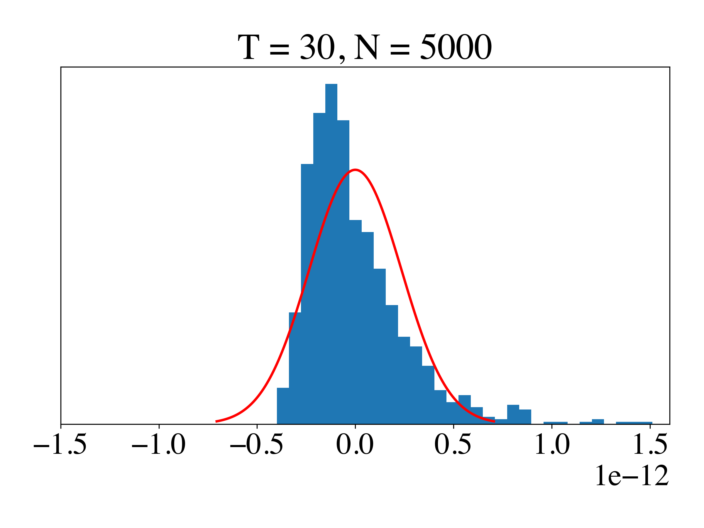
We conducted a series of experiments to validate theorem 1. We simulated a target series $x_{1:T}$ with $x_{i}\in\mathbb{R}^{3}$ and $T=\{30,100\}$ using a 3-state GHMM, where the initial probabilities and sticky transition probabilities are as described in Section 5.1.1. We set the discrete emission probability matrix to $[[0.8,0.1,0.1]^{\top},[0.1,0.8,0.1]^{\top},[0.1,0.1,0.8]^{\top}]^{\top}$. We estimated parameters $\widehat{\mu},\widehat{\Sigma}$, and $\widehat{K}$ using training samples generated from the same model as the target series. Specifically, $N$ i.i.d. samples $Y_{1}^{(\mu)}$ were used to estimate $\widehat{\mu}$, $N$ i.i.d. samples of $(Y_{1}^{(\Sigma)},Y_{2}^{(\Sigma)})$ to estimate $\widehat{\Sigma}$, and $N$ i.i.d. samples of $(Y_{1}^{(K)},Y_{2}^{(K)},Y_{3}^{(K)})$ to estimate $\widehat{K}$. We used training sets of size $N=5000,10000,50000,100000$, replicating the experiment 1000 times for each $N$. For each replication $r$, we estimated $\hat{P}r(x_{1:T})^{(N,r)}$ and constructed a histogram of the estimation errors $\{\hat{P}r(x_{1:T})^{(N,r)}-Pr(x_{1:T})^{(N,r)}\}_{r}$. We compared this histogram to the theoretical probability density function (pdf), which by Theorem 1 should converge to a normal distribution as $N$ increases.

In Figure 3 we see that, as $N$ increases, the distribution of the estimated likelihood converges to the normal distribution, and with a shorter length $T$, the error converges faster. We also analyzed the asymptotic behavior of the first-order estimation errors separately for the first moment, $(v+\tilde{v})^{\top}\widehat{\Delta\mu}$, second moment, $\sum_{t=0}^{T}b_{t}^{\top}\widehat{\Delta\Sigma}\tilde{b_{t}}$, and third moment, $\sum_{t=1}^{T}a_{t}^{\top}\widehat{\Delta K}(y_{t})\tilde{a_{t}}$ (see Figure 4). We found that the third moment estimation error has the largest effect, as shown in Table 1. We further analyzed the asymptotic distribution of the Frobenius norm of the first, second and third moment estimation error. Figure 5 shows the empirical histogram and its corresponding theoretical pdf.

We note two sources of error in estimating the likelihood. The first is the typical CLT-type error in parameter estimation, which decreases as $N$ increases. The second the propagation of estimation errors during forward recursion. To achieve a stable normal distribution given the second issue, $N$ must be much greater than $T$. In our simulation with $T=100$, we observe reasonable evidence of asymptotic normality at $N=10000$, but not at $N=5000$. When $N=T$ or is only slightly larger, the distribution is heavy-tailed, suggesting that regularization could be beneficial.

For simplicity of presentation, we derive Theorem 1 under the assumption that the output distribution is discrete. For continuous output, the CLT still holds with a proper kernel function $G(\cdot)$ as mentioned in section 1.2.

The Baum-Welch algorithm (Baum et al.,, 1970) predicts belief probabilities, or weights, for each underlying hidden state. Let $\hat{w}_{t}$ denote the predicted weight vector at time $t$. The prediction can be expressed as a weighted combination of cluster means: $\hat{y}_{t}=M\hat{w}_{t}$ where $||\hat{w}_{t}||_{1}=1$. In the Baum-Welch algorithm, these weights are explicitly guaranteed to be non-negative and sum to 1 during forward propagation, which is consistent with their interpretation as probabilities.

However, SHMM does not directly estimate the belief probabilities, and these constraints are not explicitly enforced in spectral estimation. Consequently, SHMM can sometimes produce predictions that are far from the polyhedron spanned by the cluster means. To address this issue, we propose the projected SHMM, where projection serves to regularize the predictions, constraining them within a reasonable range.

This is particularly important when $N$ is not sufficiently large, and extreme deviations of the estimated likelihood from the true likelihood can occur when error is propagated over time. Regularization can help stabilize the performance of estimation of the likelihood by limiting this propagation of error.

We propose two projection methods for SHMM: projection-onto-polyhedron and projection-onto-simplex. Projection-onto-polyhedron directly addresses the motivation for using projections in SHMM but is computationally expensive. As a computationally efficient alternative, we propose projection-onto-simplex.

This section addresses two key aspects of PSHMM implementation: choosing the dimensionality of the projection space and computing the projection matrix $U$.

We illustrate an online learning strategy that allows for adaptive parameter estimation. Let $\hat{\mu},\hat{\Sigma}$, and $\hat{K}$, be the estimated moments based on $T$ data points. Upon receiving new data $Y_{T+1}$, we update our moments recursively:

References

- Baum and Petrie, (1966) Baum, L. E. and Petrie, T. (1966). Statistical inference for probabilistic functions of finite state markov chains. The annals of mathematical statistics, 37(6):1554–1563.
- Baum et al., (1970) Baum, L. E., Petrie, T., Soules, G., and Weiss, N. (1970). A maximization technique occurring in the statistical analysis of probabilistic functions of markov chains. The annals of mathematical statistics, 41(1):164–171.
- Boyd et al., (2004) Boyd, S., Boyd, S. P., and Vandenberghe, L. (2004). Convex optimization. Cambridge university press.
- Dempster et al., (1977) Dempster, A. P., Laird, N. M., and Rubin, D. B. (1977). Maximum likelihood from incomplete data via the EM algorithm. J. R. Stat. Soc. Series B Stat. Methodol., 39(1):1–22.
- Eckart and Young, (1936) Eckart, C. and Young, G. (1936). The approximation of one matrix by another of lower rank. Psychometrika, 1(3):211–218.
- Frisch, (1955) Frisch, K. (1955). The logarithmic potential method of convex programming. Memorandum, University Institute of Economics, Oslo, 5(6).
- Grossman and Zhou, (1993) Grossman, S. J. and Zhou, Z. (1993). Optimal investment strategies for controlling drawdowns. Mathematical finance, 3(3):241–276.
- Halko et al., (2011) Halko, N., Martinsson, P.-G., and Tropp, J. A. (2011). Finding structure with randomness: Probabilistic algorithms for constructing approximate matrix decompositions. SIAM review, 53(2):217–288.
- Harris et al., (2020) Harris, C. R., Millman, K. J., van der Walt, S. J., Gommers, R., Virtanen, P., Cournapeau, D., Wieser, E., Taylor, J., Berg, S., Smith, N. J., Kern, R., Picus, M., Hoyer, S., van Kerkwijk, M. H., Brett, M., Haldane, A., del Río, J. F., Wiebe, M., Peterson, P., Gérard-Marchant, P., Sheppard, K., Reddy, T., Weckesser, W., Abbasi, H., Gohlke, C., and Oliphant, T. E. (2020). Array programming with NumPy. Nature, 585(7825):357–362.
- Hassan and Nath, (2005) Hassan, M. R. and Nath, B. (2005). Stock market forecasting using hidden markov model: a new approach. In 5th International Conference on Intelligent Systems Design and Applications (ISDA’05), pages 192–196. IEEE.
- Hsu et al., (2012) Hsu, D., Kakade, S. M., and Zhang, T. (2012). A spectral algorithm for learning hidden markov models. Journal of Computer and System Sciences, 78(5):1460–1480.
- Jaeger, (2000) Jaeger, H. (2000). Observable Operator Models for Discrete Stochastic Time Series. Neural Comput., 12(6):1371–1398.
- Knoll et al., (2016) Knoll, B. C., Melton, G. B., Liu, H., Xu, H., and Pakhomov, S. V. (2016). Using synthetic clinical data to train an hmm-based pos tagger. In 2016 IEEE-EMBS International Conference on Biomedical and Health Informatics (BHI), pages 252–255. IEEE.
- Lahmiri and Bekiros, (2021) Lahmiri, S. and Bekiros, S. (2021). Deep learning forecasting in cryptocurrency high-frequency trading. Cognitive Computation, 13:485–487.
- Mamon and Elliott, (2014) Mamon, R. S. and Elliott, R. J. (2014). Hidden Markov models in finance: Further developments and applications, volume II. International series in operations research & management science. Springer, New York, NY, 2014 edition.
- McLachlan and Basford, (1988) McLachlan, G. J. and Basford, K. E. (1988). Mixture models: Inference and applications to clustering, volume 38. M. Dekker New York.
- Pedregosa et al., (2011) Pedregosa, F., Varoquaux, G., Gramfort, A., Michel, V., Thirion, B., Grisel, O., Blondel, M., Prettenhofer, P., Weiss, R., Dubourg, V., Vanderplas, J., Passos, A., Cournapeau, D., Brucher, M., Perrot, M., and Duchesnay, E. (2011). Scikit-learn: Machine learning in Python. Journal of Machine Learning Research, 12:2825–2830.
- Rodu, (2014) Rodu, J. (2014). Spectral estimation of hidden Markov models. University of Pennsylvania.
- Rodu et al., (2013) Rodu, J., Foster, D. P., Wu, W., and Ungar, L. H. (2013). Using regression for spectral estimation of hmms. In International Conference on Statistical Language and Speech Processing, pages 212–223. Springer.
- Scott et al., (2005) Scott, S. L., James, G. M., and Sugar, C. A. (2005). Hidden markov models for longitudinal comparisons. J. Am. Stat. Assoc., 100(470):359–369.
- Sharpe, (1966) Sharpe, W. F. (1966). Mutual fund performance. The Journal of business, 39(1):119–138.
- Shirley et al., (2010) Shirley, K. E., Small, D. S., Lynch, K. G., Maisto, S. A., and Oslin, D. W. (2010). Hidden markov models for alcoholism treatment trial data. aoas, 4(1):366–395.
- Siddiqi et al., (2009) Siddiqi, S., Boots, B., and Gordon, G. J. (2009). Reduced-rank hidden markov models. AISTATS, 9:741–748.
- Stratos et al., (2016) Stratos, K., Collins, M., and Hsu, D. (2016). Unsupervised part-of-speech tagging with anchor hidden markov models. Trans. Assoc. Comput. Linguist., 4:245–257.
- Virtanen et al., (2020) Virtanen, P., Gommers, R., Oliphant, T. E., Haberland, M., Reddy, T., Cournapeau, D., Burovski, E., Peterson, P., Weckesser, W., Bright, J., van der Walt, S. J., Brett, M., Wilson, J., Millman, K. J., Mayorov, N., Nelson, A. R. J., Jones, E., Kern, R., Larson, E., Carey, C. J., Polat, İ., Feng, Y., Moore, E. W., VanderPlas, J., Laxalde, D., Perktold, J., Cimrman, R., Henriksen, I., Quintero, E. A., Harris, C. R., Archibald, A. M., Ribeiro, A. H., Pedregosa, F., van Mulbregt, P., and SciPy 1.0 Contributors (2020). SciPy 1.0: Fundamental Algorithms for Scientific Computing in Python. Nature Methods, 17:261–272.
- Wang and Carreira-Perpinán, (2013) Wang, W. and Carreira-Perpinán, M. A. (2013). Projection onto the probability simplex: An efficient algorithm with a simple proof, and an application. arXiv preprint arXiv:1309.1541.
- Zhou and Su, (2001) Zhou, G. and Su, J. (2001). Named entity recognition using an HMM-based chunk tagger. In Proceedings of the 40th Annual Meeting on Association for Computational Linguistics - ACL ’02, Morristown, NJ, USA. Association for Computational Linguistics.