Bridging The Multi-Modality Gaps of Audio, Visual and Linguistic for Speech Enhancement
Abstract
Speech Enhancement (SE) aims to improve the quality of noisy speech. It has been shown that additional visual cues can further improve performance. Given that speech communication involves audio, visual, and linguistic modalities, it is natural to expect another performance boost by incorporating linguistic information. However, bridging the modality gaps to efficiently incorporate linguistic information, along with audio and visual modalities during knowledge transfer, is a challenging task. In this paper, we propose a novel multi-modality learning framework for SE. In the model framework, a state of the art diffusion Model based backbone is utilized for Audio-Visual Speech Enhancement (AVSE) modeling where both audio and visual information are directly captured by microphones and video cameras. Based on this AVSE, the linguistic modality employs a PLM to transfer linguistic knowledge to the visual-acoustic modality through a process termed Cross-Modal Knowledge Transfer (CMKT) during AVSE model training. After the model is trained, it is supposed that linguistic knowledge is encoded in the feature processing of the AVSE model by the CMKT, and the PLM will not be involved during inference stage. We carry out SE experiments to evaluate the proposed model framework. Experimental results demonstrate that our proposed AVSE system significantly enhances speech quality and reduces generative artifacts, such as phonetic confusion compared to the state-of-the-art. Moreover, our visualization results demonstrate that our Cross-Modal Knowledge Transfer method further improves the generated speech quality of our AVSE system. These findings not only suggest that Diffusion Model-based techniques hold promise for advancing the state-of-the-art in AVSE but also justify the effectiveness of incorporating linguistic information to improve the performance of Diffusion-based AVSE systems.
Index Terms:
Diffusion Model, Predictive and Generative model, Audio-Visual Speech Enhancement, Pretrained Language model (PLM), Cross-Modal Knowledge Transfer.I Introduction
Deep learning (DL) has rapidly become a powerful tool in the field of Speech Enhancement (SE), leading to remarkable progress. By utilizing deep architectures, DL models can capture complex features from noisy input signals, allowing for the effective reconstruction of clean speech. Several DL-based models have been applied to SE, including deep denoising autoencoders (DDAEs) [1], fully connected neural networks (FCNNs) [2], convolutional neural networks (CNNs) [3], and recurrent neural networks (RNNs) with long short-term memory (LSTM) units [4]. These approaches have proven to consistently outperform both traditional SE methods and earlier machine learning techniques.
A major benefit of deep learning (DL) models is their ability to combine data from various domains. With many devices capable of capturing both audio and visual information simultaneously, recent research has explored incorporating visual cues to enhance speech enhancement (SE) systems, a technique known as Audio-Visual Speech Enhancement (AVSE). Traditional SE methods, which depend solely on audio input, are prone to difficulties like background noise and overlapping speech. In contrast, AVSE integrates visual information, such as lip movements and facial expressions, to complement the auditory signals, leading to more precise speech reconstruction. Several AVSE and Audio-Visual Speech Separation (AVSS) systems have been developed and proven effective [5] [6] [7] [8] [9] [10] [11] [12] [13] [14] [15] [16]. Some unified learning frameworks also proposed to jointly learn Audio-Visual Speech Enhancement with another task [17].
Recently, Diffusion Models [18] have been introduced and shown to be competitive in both vision and speech regression tasks. [19] proposed a Diffusion-based SE model that incorporates a supervised training loss component alongside a generative Gaussian noise prediction loss, demonstrating the effectiveness of a Diffusion-based SE system. Additionally, [20] presented an Audio-Visual Speech Separation (AVSS) system that employs a Diffusion model in two stages: a Predictive stage and a Generative stage, achieving state-of-the-art results across several benchmarks.
Speech communication relies on multiple modalities, including audio, visual, and linguistic elements, so it is logical to expect that incorporating linguistic information could further enhance the performance of SE. In noisy environments with human interference, integrating linguistic knowledge allows the SE model to identify context-dependent relationships between textual content and the target speaker’s utterances, leading to clearer speech and enhanced overall performance.
Incorporating a pretrained language model (PLM) offers a potential solution for linguistic-guided AVSE. After aligning features across different modalities, the PLM refines visual-acoustic feature representations using linguistic-guided loss functions. However, the feature distributions of visual-acoustic and linguistic modalities vary significantly. Directly forcing high similarity between these features could lead to a loss of important visual-acoustic information. These domain gaps make transferring linguistic knowledge in AVSE more challenging.
In this study, we propose a Diffusion-based AVSE system integrating visual, acoustic, and linguistic modalities. The visual-acoustic component employs both a Predictive stage and a Generative stage to produce clean speech from noisy audio and lip movements. Additionally, we introduce a linguistic framework that leverages context-dependent knowledge from a Pre-Trained BERT Model (PLM) to train the AVSE system, referred to as ”Linguistic Cross-Modal Knowledge Transfer (LCMKT).” This framework is implemented in two ways: ”Multi-Head Cross-Attention (MHCA)” [21] and ”Optimal Transport (OT)” [22]. Both methods facilitate the transfer of linguistic knowledge between visual-acoustic and linguistic modalities by bridging the domain gaps between them. Moreover, since this linguistic framework is only applied during training, the additional inference cost is nearly zero, demonstrating its efficiency in terms of parameters and computation. Our experiments, conducted on the Chinese ”Taiwan Mandarin Speech with Video (TMSV)” dataset and the English ”3rd AVSE Challenge Dataset,” not only validate the effectiveness of our proposed AVSE system but also highlight the significant benefits of incorporating the linguistic modality in the AVSE task.
II Related Works
Recently, through an analysis of the stochastic differential equation (SDE) tied to the discrete-time Markov chain [23], diffusion models have been associated with score matching [24]. This connection allows the forward process to be reversed, producing a corresponding reverse SDE that depends solely on the score function of the perturbed data [25]. [26] proposed a Speech Enhancement (SE) system utilizing Score-Based Diffusion Model, which defines forward and reverse processes by Stochastic Differential Equations (SDE). This work extends the Score-Based Generative Modeling from [23]. In our study, we refer to the Score-Based Diffusion Model and feature-preprocessing steps proposed by [26] in our Visual-Acoustic modality.
Recent studies have increasingly acknowledged the advantages of using the PLM to transfer context-dependent linguistic knowledge, which boosts the capability of acoustic models for speech classification tasks (ex: speech recognition). This knowledge transfer process is termed “Linguistic Cross-Modal Knowledge Transfer (LCMKT)”. [27] utilize a pre-trained language model with Optimal Transport (OT) to boost an end-to-end Connectionist Temporal Classification(CTC)-based Audio Speech Recognition (ASR) framework. [28] utilize hierarchical architecture with Sinkhorn Attention [29] to further boost the performance of CTC-OT ASR framework. To investigate whether LCMKT can also transfer linguistic knowledge by bridging the domain gaps on AVSE tasks, we include LCMKT in the training stage of our proposed system.
We also review several existing AVSE systems on TMSV Dataset. AVDCNN [5] incorporates audio and visual streams into a unified network model and propose a multi-task learning framework for Audio Visual Speech Enhancement. iLAVSE [30] uses convolutional recurrent neural network architecture as the backbone model, which validated the effectiveness of incorporating visual input to improve Speech Enhancement(SE) performance. Moreover, iLAVSE utilizes the mouth region of interest (ROI) rather than the entire face for a more efficient AVSE system. AVCVAE [31] proposes audio-visual variants of Variational auto-encoders (VAE) for single-channel and speaker-independent speech enhancement. SSL-AVSE [32] leverage AV-Hubert [33] to combine visual cues with audio signals. DCUC-Net [34] design a complex U-Net-based framework leveraging complex domain features and a stack of conformer blocks, which is the SOTA on TMSV Dataset. On the other hand, we also compare our results with several benchmark models on the 3rd AVSE Challenge. MMDTN [35] presents a multi-model dual-transformer that uses the attention mechanism to capture correlations between features for AVSE. LSTMSE-Net [36] proposed long short-term memory network processing visual and audio features through a separator network for optimized AVSE, These works serve as our baseline model for comparison in the later section.

III Proposed method
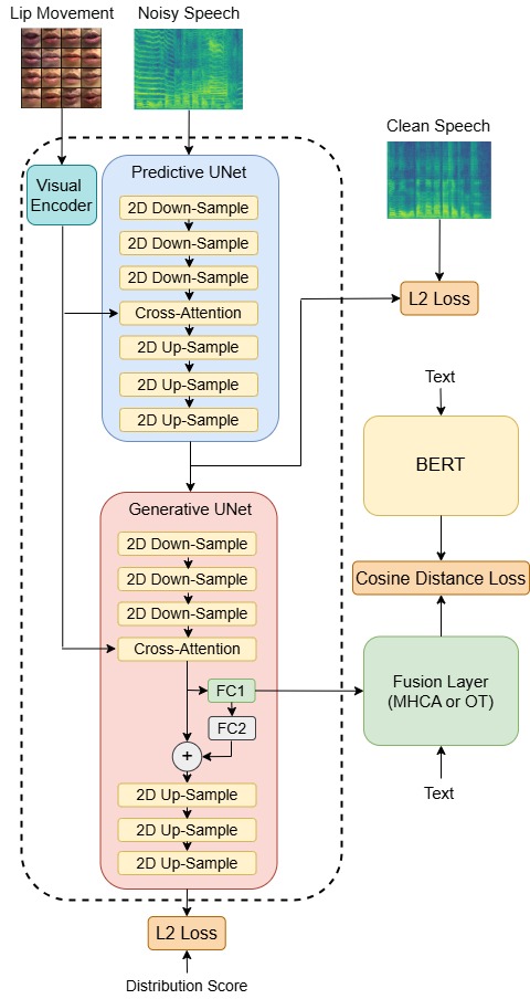
In this work, we adapt the hybrid Diffusion AVSE System system “DAVSE” [37]. This work extends the application of diffusion models [38] to the audio-visual domain by injecting visual information into the diffusion process. We further extend this AVSE system to three modalities, including acoustic modality, visual modality, and linguistic modalities. Our model can be divided into two branches. The overall AVSE training architecture can be seen in Fig. 1.
The left branch represents acoustic modality and visual modality, which consists of a Predictive model and a Generative model. The Predictive model serves as a preliminary noise predictor, which pre-processes the input noisy speech spectrogram and the visual embeddings, and the outputs serve as a guide for the diffusion process. For the Generative model, the inputs will be the preliminary-denoised speech spectrogram, the current process state spectrogram with a specific timestep, and the visual embeddings. The output will be the score of the distribution at each intermediate time step. This Generative model is also called a “score model”. For both Predictive and Generative models, we use cross-attention blocks to integrate visual and acoustic modalities.
The right branch represents linguistic modality, which consists of a pre-trained language model “BERT” [39] and a cross-modal alignment model. To force the acoustic model to encode context-dependent linguistic information, we use text embeddings and the intermediate feature in our Generative model as the inputs of the cross-alignment model. This model can be either “Cross-Attention” or “Optimal Transport”, which aims to transfer the linguistic knowledge encoded in BERT to the visual-acoustic model by adding additional distance loss. This enables our visual-acoustic feature to behave somehow like the BERT’s linguistic feature. However, since the feature distribution and feature dimension are quite different between the visual-acoustic feature and linguistic feature, we cannot directly transfer linguistic knowledge by the original visual-acoustic feature in our Generative model. To solve the problem of domain gap, we design a cross-modal neural adapter, which consists of a fully connected layer and a feedback addition. This adapter is attached to visual-acoustic modality for effective linguistic knowledge transfer. The final intermediate feature representation in our Generative model is an addition of the original feature and the output of the cross-modal neural adapter. We supposed that the feature explored by these two-branch modalities will boost the linguistic information representation for AVSE. At the inference stage, we adapt the idea of a hybrid Diffusion System proposed by [20]. The overall Diffusion process can be seen in Fig. 2.
III-A Lip Movement Model
Instead of using the visual information of the entire human face, we use mouth Region-Of-Interest (ROI). These lip movements enable our visual model to focus on the most relevant visual information on the human face and improve the accuracy of AVSE. To extract the feature of visual modality, we utilize a modified ResNet-18 [40] visual encoder pre-trained on the Lip Reading in the Wild dataset (LRW), where the mouth ROI encoder consists of a 3D convolutional layer that processes consecutive frames, followed by a 2D ResNet-18. The output features of the visual encoder will be sent into the following Predictive and Generative models as visual embeddings. Note that since we freeze this visual encoder during our training stage, we can extract the visual embeddings of all the datasets beforehand. It means that we don’t need to include the visual model during our entire training stage, which reduces parameters and memory usage.
| (1) |
Where is the lip movement model, is the visual embeddings, and is the image of ROI.
III-B Predictive Denoiser Model
Since the initialization of the diffusion process significantly affects the enhanced speech of the Generative model, we utilize a Predictive denoiser to provide an initial estimation of noise. The noisy speech is initially converted into a spectrogram using the short-time Fourier transform (STFT) and serves as an input to this model, and the output of this model will then be sent into the Generative model. As a guide for the diffusion process, we assume that this initial estimation will improve the later diffusion process and provide a higher-quality enhancement result. In this study, we use the same model architecture as our Predictive denoiser, which will be further described later.
| (2) |
Where is the Predictive denoiser, is the noisy speech spectrogram and is the preliminary-denoised speech spectrogram.
To train this denoiser, we apply a Mean square error (MSE) Loss between the denoised speech spectrogram and the clean speech spectrogram.
| (3) |
Where is the loss of the Predictive denoiser, is the clean speech spectrogram.
III-C Generative Score-Based Diffusion Model
In the Generative part of the acoustic modality, we adopt a score-based diffusion model “SGMSE” proposed by Richter et al. [26]. “SGMSE” defines the diffusion process in the complex short-time Fourier transform (STFT) domain, which uses Stochastic Differential Equations (SDE) to operate speech spectrograms. In the forward process, noise is gradually added to the clean speech spectrogram, which is described by the Stochastic Differential Equation (SDE):
| (4) |
Where is the spectrogram of the current process state, is a continuous time-step variable describing the progress of the process. Note that since we use the predictive model before the diffusion process, preliminary-denoised speech spectrogram is used here, and denotes a standard Wiener process.
Functions and represent “drift coefficient” and “diffusion coefficient” respectively. The definitions of them are given below:
| (5) |
| (6) |
Where is a constant called “stiffness”, which controls the transition from x0 to y. and are parameters defining the noise schedule of the Wiener process.
While the reverse process learns to generate a clean speech spectrogram in an iterative way starting from the preliminary-denoised speech. This process is described by another SDE:
| (7) |
where is “score” approximated by a DNN. This DNN is therefore called the score model. We can then denote the score model as , which is determined by model parameters in DNN and receives the current process state , the preliminary-denoised speech spectrogram , and the current time-step as inputs. After plugging in , our SDE of the reverse process can be rewritten as:
| (8) |
After training the score model, we can use the output of the score model to plug in reverse SDE, and this equation can be solved by various discrete solver procedures.
At the inference stage, we can use the well-trained model to iterate through the reverse process from to . The initial condition of the reverse process at is given below:
| (9) |
Where initial condition is sampled from , which denotes the circularly symmetric complex normal distribution, and denotes the identity matrix. Following the denoising process, the enhanced spectrogram is converted back to a waveform using the inverse short-time Fourier transform (ISTFT).
At each training step, we sample and pass into the score model . The sampling procedure can be summarized as: (1) Sample timestep (2) Sample from the dataset (3) Sample (4) Sample by the equation:
| (10) |
Where and denote the mean and variance of Gaussian process. Since the initial conditions are known, we can derive the equations for them:
| (11) |
| (12) |
Where is the clean speech. To explicitly define the objective function at the training stage, we use denoising score-matching to rewrite the approximated score as:
| (13) |
By substituting Eq. (10) into Eq. (13), our overall training objective can be defined as an L2 loss:
| (14) |
III-D Visual-Acoustic Fusion
Inspired by Stable Diffusion [42], which demonstrates that cross-attention is effective in injecting the conditions from various input modalities for conditional image generation, we’re interested in using cross-attention blocks to integrate visual-acoustic information. For the self-attention blocks in our Predictive and Generative acoustic models, we replace the acoustic key and value with the visual embedding encoded by our visual encoder. We assume that complementing the acoustic input with visual lip movement information leads to more accurate speech reconstruction. The overall performance of the speech enhancement system can be boosted without additional cost.
| (15) |
Where is the visual-acoustic feature, and is the original acoustic feature in the Predictive or Generative model.
III-E Audio Text Generation
To enable the training of linguistic knowledge transfer, we utilize the speech recognition model Whisper [43] to generate the text for each clean speech. Note that we use the large model for higher recognition accuracy.
III-F Linguistic Feature Representation
In the right branch of Fig. 1, the context-dependent linguistic representation is explored from a pre-trained BERT model. The output of this BERT model is termed linguistic guidance, which helps visual-acoustic modality learn the context-dependent representation. The process of extracting linguistic guidance can be formulated as:
| (16) |
Where “” is the text sequence generated by Whisper [43], “” is word piece-based tokens “” is a pre-trained BERT model, token symbols “CLS” and “SEP” represent the start and end of an text sequence, is the linguistic guidance which encodes context-dependent linguistic information, denotes the text sequence length, and denotes the token-based vocabulary size.
III-G Cross-Modal Knowledge Transfer
By using Cross-modal knowledge transfer (CMKT), we can force the visual-acoustic model to encode context-dependent linguistic information. This is achieved by introducing additional losses from the linguistic modality, which closes the distance between visual-acoustic features from the left branch and linguistic guidance from BERT. However, the dimension and distribution are quite different between visual-acoustic feature and linguistic guidance . To solve the problem of this huge domain gap, we adopt the concept of “Cross-Modal Alignment” and “Cross-Modal Neural Adapter” proposed by Lu et al.[27] in our CMKT system.
Cross-Modal Alignment consists of a fully connected layer and one of the feature fusion layers, which aims to transfer linguistic knowledge from BERT to our visual-acoustic modality. To achieve this, we force the fusion of the encoded-text embedding and visual-acoustic latent features to behave like our linguistic guidance from BERT. However, since the feature dimension is different between visual-acoustic features and encoded text embedding, a fully connected layer is used to project visual-acoustic features into the visual-acoustic latent features as:
| (17) |
Where is the visual-acoustic feature from the encoder output of the Generative model, is the visual-acoustic latent feature, which has the same dimension as encoded text embedding, denotes the length of the visual-acoustic feature, and represents feature dimension of text representation.
In this study, we implement two types of fusion layers models, termed “Multi-Head Cross-Attention (MHCA)” and “Optimal Transport (OT)” respectively. Both of them aim to fuse the information from visual-acoustic and information from linguistic modality.
For Multi-Head Cross-Attention (MHCA), we fuse the feature by multiple cross-attention layers [21]. The extraction of encoded-text embedding is:
| (18) |
Where is text embedding from the tokenizer, is a token embedding layer, and is position encoding of text embedding. In each cross-attention layer, the transform is formulated as:
| (19) |
Where “MHCA” denotes the multi-head cross-attention layer, and “” is the index of the layer with values from 1 to . After cross-attention layers, we apply a layer norm and a linear transform, the context-dependent visual-acoustic feature (Cross-Modal Embedding) can be obtained from:
| (20) |
Where “LN” denotes layer norm, “” is a full-connected linear transform and “” denotes the token-based vocabulary size.
Optimal Transport (OT) is another fusion process. The original OT is proposed by Villani et al.[22], which transports a distribution to another with the minimum amount of cost. Lu et al.[27] use this concept for CMKT and prove that OT is successful in Speech Recognition. We adopt a similar concept, which finds the optimal transport matching between visual-acoustic modality and linguistic modality. This projection matrix will then be used for efficient projection between two feature spaces. In the training process, this projection matrix is obtained by an OT Loss defined below:
| (21) |
Where is the OT Loss for finding an optimal transport matrix, is a transport plan matrix, is a set of transport plan between two distributions, is a transport cost between and , where and are column vectors in
and respectively. Note that the inputs of this loss function are text embedding from the tokenizer and visual-acoustic latent features. For simplification, we denote as , as in this equation.
The transport cost is explicitly defined as a cosine distance function below:
| (22) |
The optimal transport plan matrix can be obtained by minimizing OT Loss:
| (23) |
To solve this equation, we adopt the “Sinkhorn Attention” proposed by Tay et al.[29] and C. Villani et al. [22]. Minimizing OT Loss by Sinkhorn Attention proves to be successful on Speech Recognition tasks by Lu et al.[28]. We can obtain the final optimal transport plan matrix by the transport cost and projection process, which can be implemented as:
| (24) |
Where and in Eq. (22) define the initial condition of transport coupling. is the transport coupling at the current iteration process, and are column-wise and row-wise normalization respectively. The normalization processes are formulated as:
| (25) |
After several iteration processes, we obtain the optimal transport plan matrix, and the context-dependent visual-acoustic feature (Cross-Modal Embedding) can be estimated from:
| (26) |
To further refine the feature representation in our Generative model, Cross-Modal Neural Adapter is attached to the Generative model in the left branch, which is represented by another fully connected layer. The linear transform can be defined as:
| (27) |
Where is the visual-acoustic projected feature, is a fully-connected linear transform and denotes the dimension of visual-acoustic feature. As the output of , will be sent into Cross-Modal Alignment for knowledge transfer, and we assume that after the training stage, it contains context-dependent information from the linguistic modality. After projecting back to the visual-acoustic feature space, helps visual-acoustic features to encode context-dependent information. This feature refinement further boosts the feature representation in the Generative model. The process can be formulated as:
| (28) |
Where “” is a weighting coefficient of Cross-Modal Neural Adapter, which controls how much linguistic knowledge from the linguistic modality can affect the visual-acoustic representation in the Generative model. The new representation of the visual-acoustic feature will then be sent into the Up-sampling layers of the Generative UNet for the later diffusion process. (subscript ‘t’ denotes visual-acoustic features incorporating linguistic modality).
In the training stage, we force the visual-acoustic modality encoding context-dependent information by an additional Cross-Modal Alignment Loss. This loss can be estimated by the cosine distance function given below:
| (29) |
Where “” denotes the Cross-Modal Alignment loss. By minimizing the cross-modal transfer loss defined in Eq. (29), we suppose that feature representation in visual-acoustic modality encodes rich linguistic information.
For AVSE with MHCA, given speech spectrograms (including a noisy one and a clean one), lip movement, and corresponding text token sequence, we can train an AVSE system with Linguistic Cross-Modal Knowledge transfer with the total loss defined as:
| (30) |
Where is the loss of Predictive model, is the loss of Generative score model, is Cross-Modal Alignment loss defined in Eq. (29), weights Generative model loss and Predictive model loss, weights Cross-Modal Alignment. For AVSE with OT, we aim to find an optimal transport matrix between two distributions. To achieve this, we introduce an additional OT Loss in our total loss, which is defined below:
| (31) |
Where is OT Loss defined in Eq. (21). After the model is trained, only the left branch of our AVSE system (see Fig. 1) is kept for inference, which saves the parameters and computing costs.
IV Experiments
In this section, we introduce our model implementation and evaluate our proposed AVSE system with Cross-Modal Knowledge Transfer. We compare the performance of our model with several benchmark models on two datasets. To further examine whether our CMKT can improve the Speech Enhancement(SE) system, we also conduct ablation studies, which compare the results with the audio model without CMKT.
IV-A Dataset
Our experiments are conducted on Taiwan Mandarin speech with video (TMSV) dataset and 3rd AVSE Challenge [44] dataset extracted from The Lip Reading Sentences 3 (LRS3). TMSV dataset includes speech recordings from 18 native Mandarin speakers (13 males and 5 females). Each speaker recorded 320 Mandarin sentences with each sentence consisting of 10 Chinese characters. The total duration of each utterance ranges from approximately 2 to 4 seconds. To ensure methodological congruence and experiment reproducibility, we followed the procedures detailed in [30] for the introduction of noise interference into the dataset and train-test split. The 3rd AVSE Challenge dataset contains the speech from 37823 speakers, and each speaker with a 2-10 seconds video. For simplicity, we abbreviate this dataset as “LRS3” in the later sections.
IV-B Model implementation
For visual feature extraction, we utilize the Mediapipe [45] face tracker to identify facial landmarks. The final visual crop is a mouth ROI region with size of 96 × 96. Note that each frame is also normalized by the mean and standard deviation of the training set.
For acoustic feature-preprocessing, we follow the experiment settings in “SGMSE”[26]. We use a sampling rate of 16 kHz to convert audio recordings into a complex-valued STFT representation using a window size of 510, resulting in F = 256, and a periodic Hann window, hop length is 128 for TMSV and 160 for LRS3. Moreover, the length of each spectrogram is trimmed to T = 256 STFT time frames to enable multiple examples for batch training with randomly selected start and end times.
For the Predictive model, we adopt and modify NCSN++ in [23]. Since the network is originally used for generative purposes, the timestep is set to 1 and the output score of the model serves as the preliminary-denoised speech spectrogram. For the model architecture of the UNet, please refer to the original paper.
For the Generative model, we also adopt and modify NCSN++ in [26] as our backbone model. For the Stochastic Process, we set = 0.05, = 0.5, and = 1.5. We track an exponential moving average of the DNN weights with a decay of 0.999 to be used for sampling. Note that the input spectrograms are all represented in the complex STFT domain. Since NCSN++ only works with real value, the real parts and imaginary parts of the complex inputs are separated into different channels before being sent into the model. After that, the real value channels and imaginary value channels will be concatenated back as complex outputs before calculating loss.
For the sampler used in the inference stage, we use a Predictor-Corrector (PC) Sampler with reverse steps 30, which includes a Reverse Diffusion Predictor (RDP) and an Annealed Langevin Dynamics (ALD) corrector with corrector steps 1.
In the linguistic modality, we use the pre-trained checkpoints “bert-base-chinese” for TMSV, and “bert-base-cased” for LRS3. Both models from huggingface [46] are fine-tuned in our task. In our BERT model, there are transformer encoders. Token-based vocabulary size is 21128 for TMSV and 28996 for LRS3, and the dimension of the linguistic feature representation is . Since the dimension of visual-acoustic features is after downsampling in our Generative model, the fully-connected transform in Fig. 1 is a weight matrix in order to match feature dimensions between visual-acoustic and linguistic modalities. Similarly, is a weight matrix that transforms the visual-acoustic latent features back to the feature size of visual-acoustic space. For MHCA, we use attention layers with = 6, and each layer is a 4-head multi-head cross-attention layer. is 0.5, is 0.2 in Eq. (30) For OT, is 0.5, is 0.01 in Eq. (31), is 0.5 in (24). The weighting coefficient of cross-modal neural adapter is 0.1 in Eq. (28). For training configuration, we use the Adam optimizer with a learning rate of and batch size of 1.
IV-C Results
After training the entire AVSE system, only the left branch (visual-acoustic modality) in Fig. 1 will be used for inference. It means that we don’t need any text inputs to do inference. Moreover, compared to the system without CMKT, we only need two additional fully connected layers to enhance speech.
We first examine the effectiveness of using visual modality and linguistic modality to benefit speech regression tasks. We expect that the visual and linguistic information serves as the additional hint for the acoustic model and thus has better performance. We first compare the results of three types of models on TMSV dataset. All of them are based on our proposed method. The results of them are shown in Table I.
| Method | Modality | PESQ | STOI | SI-SDR |
|---|---|---|---|---|
| Noisy | - | 1.19 | 0.60 | -5.5 |
| Ours | A | 1.54 | 0.69 | 1.4 |
| Ours | A+L | 1.66 | 0.70 | 1.9 |
| Ours | A+V+L | 1.74 | 0.72 | 4.1 |
Where “Noisy” represents the original noisy input, “A” represents that we don’t integrate visual embeddings and Cross-Modal Knowledge Transfer into our AVSE system and train the model with speech ground truth only (pure acoustic model). “A+L” represents that we don’t integrate visual embeddings but enable Cross-Modal Knowledge Transfer with acoustic loss and linguistic Loss. “A+V+L” represents our proposed full AVSE framework with Cross-Modal Knowledge Transfer. In this table, we can first observe that incorporating linguistic modality can significantly benefit the original acoustic model. That’s why “A+L” surpasses “A” on TMSV. Moreover, we can include visual modality to further improve the performance of the model, and therefore “A+V+L” yields the best result.
We then compare the results our AVSE system with other benchmark models on TMSV and LRS3. The results of them are shown in Table II and Table III respectively.
| Method | Modality | PESQ | STOI | SI-SDR |
|---|---|---|---|---|
| Noisy | - | 1.19 | 0.60 | -5.5 |
| AVCVAE [31] | A+V | 1.34 | 0.63 | - |
| SSL-AVSE [32] | A+V | 1.4 | 0.68 | - |
| ILAVSE [30] | A+V | 1.41 | 0.64 | - |
| DCUC-Net [34] | A+V | 1.41 | 0.66 | - |
| Ours | A+V | 1.74 | 0.71 | 2.5 |
| Ours (+MHCA) | A+V+L | 1.74 | 0.72 | 4.1 |
| Ours (+OT) | A+V+L | 1.66 | 0.69 | 2.5 |
| Method | Modality | PESQ | STOI |
|---|---|---|---|
| Noisy | - | 1.46 | 0.61 |
| Baseline | A+V | 1.49 | 0.62 |
| LSTMSE-Net [36] | A+V | 1.55 | 0.65 |
| MMDTN [35] | A+V | 1.73 | 0.69 |
| Ours | A+V | 1.91 | 0.68 |
| Ours (+MHCA) | A+V+L | 1.82 | 0.66 |
| Ours (+OT) | A+V+L | 1.94 | 0.69 |
In these tables, the model performance was mainly evaluated based on the Perceptual Evaluation of Speech Quality (PESQ), Short-Time Objective Intelligibility (STOI), and Scale-invariant Signal-to-Distortion Ratio (SI-SDR). Moreover, we also examine the modalities used in each model, where “A” represents acoustic modality, “V” represents visual modality, and “L” represents linguistic modality.
For our method, “Ours” represents our AVSE system without Cross-Modal Knowledge Transfer, “Ours (+MHCA)” represents our AVSE system with MHCA, and “Ours (+OT)” represents our AVSE system with OT. “Baseline” represents the baseline model in the 3rd AVSE Challenge [44]. Table II shows that the AVSE system with MHCA surpasses all the other SOTA on TMSV datasets. On the other hand, Table III shows that AVSE system with OT surpasses the 3rd AVSE Challenge baseline model and several benchmark models on LRS3 datasets. These tables not only justify the effectiveness of our AVSE system but also show that Cross-Modal Knowledge Transfer enables the visual-acoustic model to learn linguistic knowledge during the training stage and therefore contributes to the improvement of the AVSE system.

To further investigate the effect of adding linguistic modality, we also performed spectrogram analysis on noisy speech, clean speech, and enhanced speech generated by our proposed model. We visualize an example in the development set on TMSV. The visualized spectrograms can be seen in Fig.3. Where “Acoustic”, “Acoustic + Linguistic”, “Acoustic + Visual”, and “Acoustic + Visual + Linguistic” is the modality model used by the model. At the end of the clean speech spectrogram, the power of the low-frequency component is much smaller. This is because the speaker stops to utter at this moment. The visualization results show that “Acoustic + Linguistic” has better noisy compression capability than “Acoustic” at the end of the speech. The reason is probably that word-based tokens help the model build the correspondence between the frequency frames and the word sequence. This additional token information serves as a hint for the model to identify the difference between pure noise and noisy word utterance. It enables the model to generate enhanced frames with lower power at the end of the speech, which is closer to the clean ground truth. Therefore, “Acoustic + Linguistic” gives better results.
Moreover, we can see that the high-frequency component is much smaller in the clean speech spectrogram. This is because the human voice mainly concentrates on the low-frequency components. The visualization results show that “Acoustic + Visual + Linguistic” has better noise compression than “Acoustic + Visual” on the high-frequency components. The reason is probably that word-based tokens help the model build the correspondence between the frequency frames and the word sequence. This additional token-frame correspondence serves as a hint for the clean word utterance at each moment. It enables the model to generate enhanced frames closer to the clean ground truth. Therefore, “Acoustic + Visual + Linguistic” gives a better result. The visualization results also show that “Acoustic + Visual + Linguistic” is the best among all settings. Our proposed method effectively suppresses the noise components present in the noisy speech spectrogram, which justifies the noise reduction capability of our model.
IV-D Ablation study
In this study, we adopt two models in our Cross-Modal Knowledge Transfer. One is the Cross-Modal Neural Adapter, which corresponds to the gray part in the Generative UNet in Fig. 1 and the other is Cross-Modal Alignment, which corresponds to the green parts in Fig. 1. To examine the effectiveness of these two methods, we conduct two additional experiments. In the first experiment, we attach the Cross-Modal Neural Adapter to the acoustic model and train this model with acoustic loss only (without CMKT). In the second experiment, we use an additional Cross-Modal Alignment model to train the ASE system with acoustic loss and linguistic loss but without attaching the Cross-Modal Neural Adapter to the acoustic model. Note that to further clarify the effectiveness of our CMKT model, we don’t integrate the visual embedding and use only the generative stage in our proposed model. It means that the Acoustic Generative model is used in this section. The results are shown in Table IV.
| Method | Modality | PESQ | STOI | SI-SDR |
|---|---|---|---|---|
| AGen | A | 1.54 | 0.69 | 1.4 |
| AGen + Adpt | A | 1.58 | 0.70 | 0.4 |
| AGen + Attn | A+L | 1.61 | 0.70 | 1.3 |
| AGen + MHCA | A+L | 1.66 | 0.70 | 1.9 |
In this table, the entry labeled “AGen” indicates the Acoustic Generative model in our system, “AGen + Adpt” indicates the Acoustic Generative model with Cross-Modal Neural Adapter (without right branch in Fig. 1), and “AGen + Attn” indicates that we apply MHCA Cross-Modal Alignment in model learning, but the adapter does not connect to the Acoustic Generative model (without and feedback addition). “AGen + MHCA” doesn’t incorporate visual information into our proposed Generative model, but enables the entire MHCA Cross-Modal Knowledge Transfer.
The results show that the “AGen + Attn” is better than the original model “AGen”. However, since it’s without attaching Cross-Modal Neural Adapter, the feature refinement in the visual-acoustic modality is limited, and that’s probably the reason why it cannot surpass the performance of “AGen + MHCA”. On the other hand, we can observe that in “AGen + Adpt”, without the context-dependent information of Cross-Modal Alignment, the linear layer with feedback addition in the UNet can not only enable knowledge transfer capability but also lead to overfitting. Therefore, although the PESQ of “AGen + Adpt” is slightly better than the original acoustic model “AGen”, the SI-SDR is significantly decreased. The result of our ablation study explains the effectiveness of using Cross-Modal Alignment and Cross-Modal Neural Adapter in our linguistic modality.
We also conduct additional experiments on the effect of selected features for CMKT. In this study, we use the visual-acoustic feature after the Cross-Attention block in UNet for CMKT. To clarify the effect of the selected feature, we conduct the following experiments in Table V.
| Selected Feature | PESQ | ESTOI |
|---|---|---|
| Down-Sample Layer | 1.98 | 0.73 |
| Cross-Attention Layer | 2.30 | 0.78 |
| Up-Sample Layer | 1.35 | 0.60 |
In this table, “Down-Sample Layer” represents that we use the feature after the second 2D Down-Sample layer, “Cross-Attention Layer” represents that we use the feature after the Cross-Attention block, and ‘Up-Sample Layer” represents that we use the feature after the last 2D Up-Sample layer in Acoustic Generative UNet. Note that we evaluate the performance of our model on TMSV Validation set. The results can also be attributed to domain gaps. In the ”Down-Sample Layer,” only a few layers are encoded with linguistic information, and this refinement is too weak to effectively bridge the domain gap. In contrast, in the ”Up-Sample Layer,” nearly all layers are linguistically encoded, causing significant information loss in the visual-acoustic domain. As a result, the ”Cross-Attention Layer” proves to be the optimal setting, explaining why we utilize the features from the Cross-Attention block for Cross-Modal Knowledge Transfer (CMKT).
IV-E Discussion
Throughout our experiments, we observed that the values of hyperparameters in Cross-Modal Knowledge Transfer have a great impact on performance improvement, especially the weight controlling loss function. To examine the importance of the parameters chosen, we plan to conduct ablation studies on the weight of Cross-Modal Alignment and the weight of Cross-Modal Neural Adapter . These two hyperparameters control the extent of domain gap bridging and significantly impact the effect of linguistic knowledge transfer. Moreover, we plan to conduct experiments on other benchmarks such as VoxCeleb2 and Lip Reading in the Wild (LRW), which further examine the generalizability of our approach. Furthermore, since it needs more parameters and computations for the linguistic guided training, we also plan to find a more compact implementation of our linguistic modality in our future study.
V Conclusion
In this study, we propose a novel Diffusion-based Audio-Visual Speech Enhancement (AVSE) system, which incorporates linguistic modality into visual-acoustic modality. Our visual-acoustic modality is based on Score-Based Diffusion model with Predictive and Generative stages and demonstrates a competitive performance on two AVSE benchmarks. For linguistic modality, we introduce two different implementations of “Cross-Modal Knowledge Transfer (CMKT)” termed ”Multi-Head Cross-Attention (MHCA)” and ”Optimal Transport (OT)”. Both of them bridge the domain gap and utilize the Pre-trained Language model “BERT” to transfer linguistic knowledge to the visual-acoustic modality. This context-dependent transferring process further improves the performance of the AVSE system without additional inference costs. Additionally, we demonstrate the effectiveness of our model on two datasets with different languages. This also implies that our proposed method is cross-language generalizable. In our future study, we not only plan to find a more compact implementation of our AVSE method but also look forward to exploring other multi-modal Speech Enhancement systems.
References
- [1] Xugang Lu, Yu Tsao, Shigeki Matsuda, and Chiori Hori, “Speech Enhancement Based on Deep Denoising Autoencoder.,” in Proc. INTERSPEECH, 2013.
- [2] Morten Kolbæk, Zheng-Hua Tan, and Jesper Jensen, “Speech Intelligibility Potential of General and Specialized Deep Neural Network Based Speech Enhancement Systems,” IEEE/ACM Transactions on Audio, Speech and Language Processing, vol. 25, no. 1, pp. 153–167, 2017.
- [3] Szu-Wei Fu, Ting-Yao Hu, Yu Tsao, and Xugang Lu, “Complex Spectrogram Enhancement by Convolutional Neural Network with Multimetrics Learning,” in Proc. MLSP, 2017.
- [4] Lei Sun, Jun Du, Li-Rong Dai, and Chin-Hui Lee, “Multiple-Target Deep Learning for Lstm-Rnn Based Speech Enhancement,” in Proc. HSCMA, 2017.
- [5] Jen-Cheng Hou, Syu-Siang Wang, Ying-Hui Lai, Yu Tsao, Hsiu-Wen Chang, and Hsin-Min Wang, “Audio-Visual Speech Enhancement using Multimodal Deep Convolutional Neural Networks,” IEEE Transactions on Emerging Topics in Computational Intelligence, vol. 2, no. 2, pp. 117–128, 2018.
- [6] Elham Ideli, Bruce Sharpe, Ivan V Baji´c, and Rodney G Vaughan, “Visually Assisted Time-Domain Speech Enhancement,” in Proc. GlobalSIP, 2019.
- [7] Ahsan Adeel, Mandar Gogate, Amir Hussain, and William M Whitmer, “Lip-Reading Driven Deep Learning Approach for Speech Enhancement,” IEEE Transactions on Emerging Topics in Computational Intelligence, pp. 1–10, 2019.
- [8] Daniel Michelsanti, Zheng-Hua Tan, Shi-Xiong Zhang, Yong Xu, Meng Yu, Dong Yu, and Jesper Jensen, “An Overview of Deep-Learning-Based Audio-Visual Speech Enhancement and Separation,” IEEE/ACM Transactions on Audio, Speech, and Language Processing, 2021.
- [9] Shang-Yi Chuang, Yu Tsao, Chen-Chou Lo, and Hsin-Min Wang, “Lite Audio-Visual Speech Enhancement,” in Proc. INTERSPEECH, 2020.
- [10] Mostafa Sadeghi, Simon Leglaive, Xavier Alameda-Pineda, Laurent Girin, and Radu Horaud, “Audio-Visual Speech Enhancement Using Conditional Variational Auto-Encoders,” in IEEE/ACM Transactions on Audio, Speech, and Language Processing, 2020.
- [11] Ariel Ephrat, Inbar Mosseri, Oran Lang, Tali Dekel, Kevin Wilson, Avinatan Hassidim, William T. Freeman, and Michael Rubinstein, “Looking to listen at the cocktail party: a speaker-independent audio-visual model for speech separation,” ACM Transactions on Graphics (TOG), 2018.
- [12] Ruohan Gao, and Kristen Grauman, “VisualVoice: Audio-Visual Speech Separation with Cross-Modal Consistency,” Proc. CVPR, 2021.
- [13] Triantafyllos Afouras, Joon Son Chung, and Andrew Zisserman, “The Conversation: Deep Audio-Visual Speech Enhancement,” in Proc.Interspeech, 2018.
- [14] Aviv Gabbay, Asaph Shamir, and Shmuel Peleg, “Visual Speech Enhancement”, in Proc.Interspeech, 2018.
- [15] E. Ideli, B. Sharpe, Ivan V. Bajić, and Rodney G. Vaughan, “Visually Assisted Time-Domain Speech Enhancement,” IEEE Global Conference on Signal and Information Processing, pp. 1–5. 2019.
- [16] A. Adeel, M. Gogate, A. Hussain, and William M. Whitmer, “Lip-Reading Driven Deep Learning Approach for Speech Enhancement,” IEEE Transactions on Emerging Topics in Computational Intelligence, vol. 5, no. 3, pp. 481–490, 2019.
- [17] Junwen Xiong, Yu Zhou, Peng Zhang, Lei Xie, Wei Huang, and Yufei Zha, “Look and listen: Multi-Modal Correlation Learning for Active Speaker Detection and Speech Enhancement,” IEEE Transactions on Multimedia, vol. 25, 2023.
- [18] Jonathan Ho, Ajay Jain, and Pieter Abbeel, “Denoising Diffusion Probabilistic Models,” NeurIPS, 2020.
- [19] Jean-Eudes Ayilo, Mostafa Sadeghi, and Romain Serizel, “Diffusion-Based Speech Enhancement with a Weight Generative-Supervised Learning Loss,” in Proc. ICASSP, 2024.
- [20] Suyeon Lee, Chaeyoung Jung, Youngjoon Jang, Jaehun Kim, and Joon Son Chung, “Seeing Through the Conversation: Audio-Visual Speech Separation Based on Diffusion Model,” in Proc. ICASSP, 2024.
- [21] A. Vaswani, N. Shazeer, N. Parmar, J. Uszkoreit, L. Jones, A. Gomez, L. Kaiser, and I. Polosukhin, “Attention Is All You Need,” in Proc. NIPS, pp. 5998-6008, 2017.
- [22] C. Villani, Optimal Transport: old and new, volume 338. Springer, 2009.
- [23] Y. Song, J. Sohl-Dickstein, D. P. Kingma, A. Kumar, S. Ermon, and B. Poole, “Score-Based Generative Modeling through Stochastic Differential Equations,” in Proc. ICLR, 2021.
- [24] A. Hyvärinen and P. Dayan, “Estimation of Non-normalized Statistical Models by Score Matching.” Journal of Machine Learning Research, vol. 6, no. 4, 2005.
- [25] B. D. Anderson, “Reverse-Time Diffusion Equation Models,” Stochastic Processes and their Applications, vol. 12, no. 3, pp. 313–326, 1982.
- [26] J. Richter, S. Welker, J.-M. Lemercier, B. Lay, and T. Gerkmann, “Speech Enhancement and Dereverberation with Diffusion-based Generative Models,” IEEE/ACM Transactions on Audio, Speech, and Language Processing, pp. 2351–2364, 2023.
- [27] Xugang Lu, Peng Shen, Yu Tsao, and Hisashi Kawai, “Cross-Modal Alignment with Optimal Transport for CTC-Based ASR,” in Proc. ASRU, 2023.
- [28] Xugang Lu, Peng Shen, Yu Tsao, and Hisashi Kawai, “Hierarchical Cross-Modality Knowledge Transfer with Sinkhorn Attention for CTC-Based ASR,” in Proc. ICASSP, 2024.
- [29] Y. Tay, D. Bahri, L. Yang, D. Metzler, and D. Juan, “Sparse Sinkhorn Attention,” in Proc. ICML, pp. 9438-9447, 2020.
- [30] S.-Y. Chuang, H.-M. Wang, and Y. Tsao, “Improved Lite Audio-Visual Speech Enhancement,” IEEE/ACM Transactions on Audio, Speech, and Language Processing, vol. 30, pp. 1345–1359, 2022.
- [31] Mostafa Sadeghi, Simon Leglaive, Xavier Alameda-PIneda, Laurent Girin, Radu Horaud, “Audio-visual speech enhancement using conditional variational auto-encoders,” IEEE/ACM Transactions on Audio, Speech, and Language Processing, vol. 28, pp. 1788–1800, 2020.
- [32] Richard Lee Lai, Jen-Cheng Hou, Mandar Gogate, Kia Dashtipour, Amir Hussain, and Yu Tsao, “Audio-Visual Speech Enhancement Using Self-supervised Learning to Improve Speech Intelligibility in Cochlear Implant Simulations,” arXiv preprint, arXiv:2307.07748, 2023.
- [33] Bowen Shi, Wei-Ning Hsu, Kushal Lakhotia, and Abdelrahman Mohamed, “Learning Audio-Visual Speech Representation by Masked Multimodal Cluster Prediction,” in Proc. ICLR, 2022.
- [34] Shafique Ahmed, Chia-Wei Chen, Wenze Ren, Chin-Jou Li, Ernie Chu, Jun-Cheng Chen, Amir Hussain, Hsin-Min Wang, Yu Tsao, and Jen-Cheng Hou, “Deep Complex U-NET with Conformer for Audio-Visual Speech Enhancement,” in 3rd COG-MHEAR Workshop on Audio-Visual Speech Enhancement (AVSEC), 2024.
- [35] Fazal E Wahab, Nasir Saleem, Amir Hussain, Rizwan Ullah, and Md Bipul Hossen, “Multi-Model Dual-Transformer Network for Audio-Visual Speech Enhancement,” in 3rd COG-MHEAR Workshop on Audio-Visual Speech Enhancement (AVSEC), 2024.
- [36] Arnav Jain, Jasmer Singh Sanjotra, Harshvardhan Choudhary, Krish Agrawal, Rupal Shah, Rohan Jha, M. Sajid, Amir Hussain, and M. Tanveer, “LSTMSE-Net: Long Short Term Speech Enhancement Network for Audio-visual Speech Enhancement,” in 3rd COG-MHEAR Workshop on Audio-Visual Speech Enhancement (AVSEC), 2024.
- [37] Chia-Wei Chen, Jen-Cheng Hou, Yu Tsao, Jun-Cheng Chen, and Shao-Yi Chien, “DAVSE: A Diffusion-Based Generative Approach for Audio-Visual Speech Enhancement,” in 3rd COG-MHEAR Workshop on Audio-Visual Speech Enhancement (AVSEC), 2024.
- [38] Y.-J. Lu, Z.-Q. Wang, S. Watanabe, A. Richard, C. Yu, and Y. Tsao, “Conditional Diffusion Probabilistic Model for Speech Enhancement,” in Proc. ICASSP, 2022.
- [39] J. Devlin, M. Chang, K. Lee, and K. Toutanova, “BERT: Pretraining of Deep Bidirectional Transformers for Language Understanding,” in Proc. NAACL-HLT, pp. 4171–4186, 2019.
- [40] P. Ma, Y. Wang, S. Petridis, J. Shen, and M. Pantic, “Training Strategies for Improved Lip-reading,” in Proc. ICASSP, 2022.
- [41] Olaf Ronneberger, Philipp Fischer, and Thomas Brox, “U-Net: Convolutional Networks for Biomedical Image Segmentation,” in Proc. MICCAI, 2015.
- [42] R. Rombach, A. Blattmann, D. Lorenz, P. Esser, and B. Ommer, “High-Resolution Image Synthesis with Latent Diffusion Models,” in Proc. CVPR, pp. 10684–10695, 2022.
- [43] https://github.com/openai/whisper
- [44] https://challenge.cogmhear.org
- [45] https://github.com/google-ai-edge/mediapipe
- [46] https://huggingface.co/