ifaamas \acmConference[AAMAS ’25] Proc. of the 24th International Conference on Autonomous Agents and Multiagent Systems (AAMAS 2025)May 19 – 23, 2025 Detroit, Michigan, USAA. El Fallah Seghrouchni, Y. Vorobeychik, S. Das, A. Nowe (eds.) \copyrightyear2025 \acmYear2025 \acmDOI \acmPrice \acmISBN \affiliation \institutionPolytechnique Montreal \cityMontreal \countryCanada \affiliation \institutionPolytechnique Montreal \cityMontreal \countryCanada \affiliation \institutionUniversity of Konstanz \cityKonstanz \countryGermany \affiliation \institutionPolytechnique Montreal \cityMontreal \countryCanada
Bridging Swarm Intelligence and Reinforcement Learning
Abstract.
Swarm intelligence (SI) explores how large groups of simple individuals (e.g., insects, fish, birds) collaborate to produce complex behaviors, exemplifying that the whole is greater than the sum of its parts. A fundamental task in SI is Collective Decision-Making (CDM), where a group selects the best option among several alternatives, such as choosing an optimal foraging site. In this work, we demonstrate a theoretical and empirical equivalence between CDM and single-agent reinforcement learning (RL) in multi-armed bandit problems, utilizing concepts from opinion dynamics, evolutionary game theory, and RL. This equivalence bridges the gap between SI and RL and leads us to introduce a novel abstract RL update rule called Maynard-Cross Learning. Additionally, it provides a new population-based perspective on common RL practices like learning rate adjustment and batching. Our findings enable cross-disciplinary fertilization between RL and SI, allowing techniques from one field to enhance the understanding and methodologies of the other.
Key words and phrases:
Swarm Intelligence, Reinforcement Learning, Evolutionary Game Theory, Opinion Dynamics1. Introduction
Swarm Intelligence (SI) takes inspiration from how a collective of natural entities, following simple, local, and decentralized rules, can produce emergent and complex behaviors Bonabeau et al. (1999). Researchers have extracted core principles such as coordination, cooperation, and local communication from these natural systems, and applied them to artificial systems, (e.g., swarm robotics Dorigo et al. (2021); Hamann (2018) and optimization algorithms Dorigo et al. (2006)).
In this paper, we focus the specific SI problem of Collective Decision Making (CDM). In CDM, individuals work together to reach an agreement on the best option from a set of alternatives, a problem commonly called the best-of-n decision problem. To solve this problem, researchers have turned to opinion dynamics Xia et al. (2011), a field that studies how opinions spread in a population. In particular, in the voter rule Castellano et al. (2009); Redner (2019), an individual copies the opinion of a randomly chosen neighbor. Similarly, researchers have taken inspiration from the house-hunting behavior of honey bees to create the weighted voter rule Valentini et al. (2014); Reina et al. (2024). In this rule, after scouting one of potential nesting areas, bees come back to perform a “dance” Visscher and Camazine (1999) that describes the coordinates of the option that they have explored. According to the weighted voter model, this dance is performed at a frequency that is proportional to the estimated quality of the explored area. Other bees go scout the area corresponding to the first dance they witness, and this process repeats until the entire colony converges to the same option.
Next, we turn toward reinforcement learning (RL), where an agent111To avoid confusion, we use “agent” in the context of RL and “individual” in the context of a population, wherever possible learns to solve a task by interacting with the environment to maximize a reward signal Sutton and Barto (2018). RL has been successfully applied to solve complex problems in various fields such as robotics Kaufmann et al. (2023), nuclear fusion Seo et al. (2024), and games Mnih et al. (2013). In this paper, we are specifically interested in multi-armed bandits Sutton and Barto (2018), in which a single agent makes choices among different options (or “arms”) to maximize its reward. Among the many learning algorithms designed to solve this task (Upper-confidence-Bound Auer et al. (2002) (UCB), -greedy Sutton and Barto (2018), Gradient Bandit Williams (1992)…), we consider the Cross Learning Cross (1973) update rule, closely related to the Gradient Bandit algorithm.
Although SI and RL are seemingly disjoint, we show that these fields can in fact be bridged via the Replicator Dynamic Sandholm et al. (2008) (RD), a famous equation used in Evolutionary Game Theory (EGT) to model the outcome of evolutionary processes through the idea of survival of fittest. In the rest of the paper, we demonstrate a mathematical equivalence between different concepts from SI and RL:
-
•
We first show that a large population whose members follow the voter rule can be seen as a single abstract RL agent following the Cross Learning update rule.
-
•
Next, via a similar argument, we show that the weighted voter rule, yields another abstract RL update that we coin Maynard-Cross Learning.
-
•
We validate these equivalences with RL and population experiments and offer a new perspective about two common practices in RL, learning rate adjustment and batching.
2. Preliminaries
2.1. Multi-armed bandits and Cross Learning
Multi-armed bandits are one of the simplest types of environments encountered in RL literature.
They consist of a discrete set of available actions, called “arms”, amongst which an agent has to find the most rewarding. In an -armed bandit, pulling arm returns a real-valued reward sampled from a hidden distribution .
The objective for an RL agent playing a multi-armed bandit is to learn a policy, denoted by the probability vector , that maximizes the rewards obtained upon pulling the arms.
Different exploration strategies exist to find such policies, one of them being Cross Learning Cross (1973):
Cross Learning (CL).
Let be an action and a corresponding reward sample (). CL updates the policy as:
| (1) |
For convenience, we denote the expected policy update on action ’s probability when sampling reward from action as:
| (2) |
In CL, every reward sampled when applying the associated action directly affects the probabilities accorded by policy to all available actions. As noted earlier, CL is closely related to the Gradient Bandit algorithm, which performs a similar update at the parameter level (called “preferences”) of a parametric policy rather than directly updating the probability vector.
2.2. Evolutionary game theory
Evolutionary game theory (EGT) studies population games Sandholm (2010).
In a single-population game, a population is made of a large number of individuals, where any individual is associated with a type, denoted by .
The population vector represents the fraction of individuals in each type (). Individuals are repeatedly paired at random to play a game, each receiving a separate payoff defined by the game bi-matrix222A bimatrix game is defined by a pair of identical-shape matrices, one per agent. . Individuals adapt their type based on these payoffs according to an update rule.333In population games, an update rule is sometimes called a revision protocol.
One notable such rule is imitation of success Sandholm (2010):
Imitation Dynamics:
Any individual of type follows the voter rule444Voter rule is not a terminology used in EGT. Instead, it comes from opinion dynamics. :
-
(1)
samples a random individual to imitate. Let be .
-
(2)
Both individuals and play the game defined by to receive payoffs and respectively (). In general, each payoff may depend on the types of both individuals.
-
(3)
switches to type with probability 555This definition of voter rule differs from opinion dynamics as individuals do not switch deterministically, but rather make a probabilistic switch..
One can easily see why this rule is called “imitation of success”: imitates based on ’s payoff. When aggregated to the entire population, imitation of success yields a famous equation in EGT, called the Taylor Replicator Dynamic Taylor and Jonker (1978); Sandholm et al. (2008) (TRD) (see Lemma 3.1):
| (3) |
where is the derivative of the -th component of the population vector , is the expected payoff of the type against the current population, and is the current average payoff of the entire population.666In Evolutionary Game Theory, expected payoffs are often referred to as “fitness”, as they model the reproductive fitness of the different types. Further, we describe another useful variant of the TRD for later convenience in the paper, the Maynard Smith Replicator Dynamic Smith (1982) (MRD):
| (4) |
2.3. Collective-decision making in swarms
Consider a population of individuals trying to reach a consensus on which amongst available options is the optimal. Similar to population games, each individual has an opinion, denoted by , about which option they prefer. We again call the population vector , which in this context represents the fraction of individuals sharing each opinion. The weighted voter rule models the dance of honey bees during nest-hunting Reina et al. (2024):
Weighted voter rule: Any individual of opinion follows the weighted voter rule :
-
(1)
estimates the quality of its current opinion , where .
-
(2)
After obtaining , locally broadcasts its opinion at a frequency proportional to .
-
(3)
switches its opinion to the first opinion that it perceives from its neighborhood. Assuming all individuals are well mixed in the population Nowak (2006), the corresponding expected probability of switching to opinion is the proportion of votes cast for : (where is the number of individuals of opinion ). This probability can further be written by dividing both the numerator and the denominator by .
Note that in this model, bees do not directly observe the quality estimate of other individuals, but only their opinion. This makes the weighted voter rule well-adapted to swarms of communication-limited organisms.
3. Theory
Remark 0.
Population-policy equivalence. As noted by Bloembergen et al. (2015), a population vector can be abstracted as a multi-armed bandit RL policy (and vice-versa). In this view, uniformly sampling an individual of type from the population is equivalent to sampling action from the policy.
3.1. Voters and Cross Learning
Proposition 1.
An infinite population of individuals following can be seen as an RL agent following Exact Cross Learning777We call ”exact” the algorithm that applies the expected update., i.e.,
| (5) |
where can be seen as both the population vector and the vector of action-probabilities under the population-policy equivalence, is the single-step change of population under the voter rule (i.e., the change in type proportions after all individuals simultaneously perform once), and is the update performed by CL on the policy for a given action-reward sample .
To prove Proposition 1, we use two intermediate results (Lemmas 3.1 and 3.1). These results are already known from the literature (although to the best of our knowledge we are the first to integrate them and apply them in this context). We provide proofs using our formalism for both Lemmas, as we will later follow a similar reasoning to prove the CDM/RL equivalence. The first result describes a policy-population equivalence between CL and the TRD:
Lemma 0.
In expectation, an RL agent learning via the CL update rule follows Bloembergen et al. (2015):
| (6) |
where is the value of action , and is the value of policy .
Proof.
Let us compute the expectation over actions sampled from in Eq. 2.
For convenience, we write
, and
:
| (7) | ||||
| (8) |
∎
The term is commonly known as the “advantage” of action in RL. From that perspective, it describes how good action is in comparison to the current policy . But Remark 3 enables looking at Lemma 3.1 under a different light: the right-hand sides of Eqs. 3 and 6 are equivalent. In other words, under the population-policy equivalence, the CL update rule tangentially follows the TRD (in expectation). Furthermore, it is known that a population adopting also yields the TRD:
Lemma 0.
Proof.
Let denote the inflow of individuals of type into type , i.e, the proportion of the population leaving type and adopting type . The population has a proportion of individuals of type , each having a probability of meeting an individual of type , and a conditional probability of switching to its type. Thus, we get :
| (10) | ||||
| (11) |
∎
Combining these results yields Proposition 1, as Lemmas 3.1 and 3.1 yield:
Proposition 1 shows how TRD connects multi-agent imitation dynamics and single-agent Exact Cross Learning. In practice, RL updates do not follow their exact expectation due to finite sampling. They rely on action samples from the policy and reward samples from the environment. To circumvent high variance and improve convergence properties, RL practitioners typically perform these policy updates in a batched fashion, which, according to Proposition 1, is equivalent to making these updates closer to infinite-population dynamics. In fact, there is an apt population-based interpretation of this practice, shown in the next section.
3.2. Learning rate and batch-size
Instead of studying the mean-field effect of aggregated individual voters, we can look at the individual effect of each voter on the entire population. This effect yields interesting insights regarding two common practices in RL: adjusting the learning rate, i.e., scaling down RL updates by a small factor, and batching, i.e., averaging RL updates over several samples.
Instead of an infinite population, let us consider a near-infinite888The assumption enables approximating flows by their expectation. population of individuals. Again, we describe by the population vector . A single individual of type sampling payoff and following has the following influence (outflow from to ) on the population vector for types :
| (12) |
while its influence on type is the sum of inflows (to ):
| (13) |
Denoting yields the following learning rule attributable to a single individual on the entire population vector:
| (14) |
Note how the RL update described in Eq. 14 differs from the one described in Eq. 1 only by a scaling factor .
The population-policy equivalence gives an interesting interpretation to the learning rate commonly used in RL. Under the population perspective, describes the number of individuals in the population. In Sec. 5, we empirically show that the CL update rule described in Eq. 1 does not typically converge to the optimal action. However, using a small enough learning rate (i.e., a large enough population size) alleviates this issue999As implied by Eq. 14, assuming that, when performed sequentially on randomly sampled individuals instead of parallelly in one step across the entire population, the voter rule still yields the Replicator Dynamic, which we conjecture. We leave a proof of this conjecture for future work..
To describe the aggregated effect of on the entire population, we can now sum the effect described in Eq. 14 across all individuals. Let us denote the payoff sampled by individual , the number of individuals of type , and the average payoff across individuals of type . The aggregated update is:
| (15) | |||||
| (16) | |||||
which is the TRD.
Note how, as a corollary of Proposition 1, summing the update from Eq. 14 over the population exactly yields the expectation of the CL update rule described in Eq. 1. By summing Eq. 14, we have retrieved the same update as what averaging Eq. 1 over a large batch would have estimated: its expectation, which is the TRD.101010As expected from the population perspective, since this derivation is essentially another proof of Lemma 3.1. From the RL perspective this result means that batching updates removes the need for using a small learning rate (see Sec. 5), at least in gradient-free multi-armed bandits where our analysis provides mathematical grounding to this commonly accepted rule of thumb.
3.3. Swarms and Maynard-Cross Learning
Arguably, the meaning of Eq. 14 is non-intuitive from the population perspective: it describes the effect of a single individual on the entire population , whereas there is no such explicit effect in . However, the weighted voter rule does contain an explicit effect, making the analysis much more intuitive.
In this Section, we will show that, similar to how imitation of success yields the CL update rule, when the entire population is considered as an abstract RL agent, swarms of bees performing CDM for house-hunting follow an abstract RL algorithm that we coin Maynard-Cross Learning.
Let us now consider a near-infinite population of honey bees, reaching a consensus on which nesting site to select via . Under , individuals have a tangible influence on the rest of the population: remember that in this model, individuals deterministically switch to the first action they witness. Hence, the influence of each individual is equal to the ratio of its broadcasting frequency , by the total broadcasting frequency of the entire population . In other words, an individual of type and payoff sample has the same influence on all other members of the population:
| (17) |
Thus, the inflow from type to type attributable to is
| (18) | ||||
| (19) |
And the total inflow into type attributable to is
| (20) | ||||
| (21) |
Eqs. 19 and 21 yield an RL update rule describing the effect of a single individual and corresponding sampled payoff (i.e., reward sample) over the entire population (i.e., policy), called:
Maynard-Cross Learning (MCL).
Let be an action and a corresponding reward sample.
MCL updates the policy as:
| (22) |
where is the current value of policy .
Finding the aggregated population effect amounts to summing Eq. 22 across all individuals:
| (23) | ||||
| (24) |
which is the MRD.
We have shown that a population whose individuals follow aggregates to the MRD. An argument similar to Sec. 3.2 yields the “batched” version of Eq. 22, that we call Exact Maynard-Cross Learning (EMCL):111111MCL has a valid implementation only when the learning rate is small enough, while EMCL has a valid implementation when the batch-size used to estimate the expectation is large enough. In both cases, also needs to be estimated.
| (25) |
EMCL is the RL algorithm followed by swarms of bees that make a collective decision via :
Proposition 2.
An infinite population of individuals following can equivalently be seen as an RL agent following EMCL
| (26) |
where is both the population vector and the policy under the population-policy equivalence, is the single-step change of population under the weighted voter rule (i.e., the change in type proportions after all individuals simultaneously perform once), and is the update performed by EMCL on the policy .
4. Methods
We present two types of experiments to validate the findings from the previous section. First, we implement the two RL update rules, CL and MCL in two variants: batched and non-batched. Second, we conduct population-based experiments using and (VR, WVR) for different population sizes. Moreover, we also numerically simulate the TRD and MRD to show how the above experiments compare with the analytical solutions.
4.1. Environment
We consider the standard multi-armed stateless bandit setting described in preliminaries (see Sec. 2.1). As it is clear from Remark 3, we can use the same environment for RL and population experiments. The environment in consideration returns rewards sampled from the hidden distribution when is pulled. A normal distribution is used to generate these reward samples, where is the mean of , and the variance. These rewards need to be bounded between , for which sigmoid function is used on , making this the hidden distribution . Moreover, this transformation squeezes and shifts the mean away from to a new mean denoted by . This can be estimated as , by sampling a large number of samples ( samples) from and averaging them. Further, three different kinds of environments are used, where ’s are near 0, spread between 0 and 1, or near 1.
4.2. RL experiments
Non-batched: In these experiments, an RL agent starts with an initial random policy . The agent then samples only one action from in an iterative fashion. Further, pulling action in the environment, the agent receives a noisy reward signal . For CL, the agent utilizes Eq. 14 to make an update. Whereas for MCL, Eq. 22 cannot be used directly, since we do not have access to . We therefore, approximate by employing a moving average over rewards, where is a weighting factor for recent rewards:
| (27) |
Moreover, since this update rule can make invalid, i.e., components could become negative or above one (see footnote 11), we clamp between 0 and 1:
| (28) |
We call this training step a run, and perform runs per seed.
Batched: In these experiments, we implement the batched variants of update rules CL (Eq. 2) and MCL (Eq. 25), henceforth named B-CL and B-MCL. B-CL is a straightforward batching of the CL update rule, averaging over a batch of samples instead of one sample to update . Whereas, with B-MCL, is no longer a moving average of the rewards but rather the mean of batch rewards. We also need to explicitly clamp the policy between 0 and 1 to ensure it remains valid. B-MCL also uses samples simultaneously similar to B-CL. Similar to non-batched experiments, we perform runs per seed.
4.3. Population Experiments
In this section, we focus on the population update rules, VR, and WVR (see preliminaries Secs. 2.3 and 2.2). Since we cannot simulate for infinite sizes, we choose two finite population sizes of 10 and 1000. For both VR and WVR, we start with an equal proportion of individuals associated with any type/opinion. Further, each individual receives a stochastic payoff/quality estimate for its type/opinion. Thereafter, with VR, everyone is paired with another random individual. All individuals then generate a random number between 0 and 1, and if the random number is greater than the payoff of the paired individual, they switch to their partner’s type (rule 3 of ). Whereas with WVR, each individual switches to an opinion sampled from the distribution defined by , where is the ratio of votes for type by the total number of votes in the population:121212We implement the third rule of in a centralized fashion for these simple numerical simulations, but in reality, it is a completely decentralized rule.
| (29) |
Similar to RL experiments, we perform runs per seed.
4.4. TRD and MRD
To empirically validate Propositions 1 and 2, we numerically simulate both the differential equations 3 (TRD) and 4 (MRD). As these equations are continuous, we discretize them by a step (discretizing step). Further, we start from an initial random population/policy () and simulate its evolution according to TRD and MRD between time intervals , using the privileged information not available to RL and population experiments.
| (30) | |||
| (31) |


Results for RL non-batched experiments for small

Results for RL non-batched experiments for large


bandits and how it connects to things

bandits and how it connects to things
5. Results
For all experiments, we use the hyperparameters described in supplementary Sec. A.3.
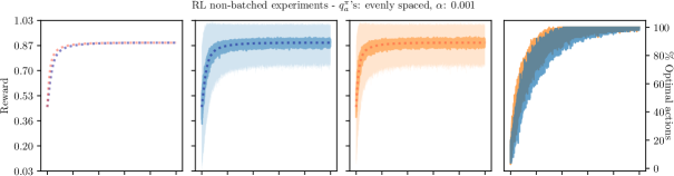
Non-batched RL update rules CL and MCL follow TRD and MRD respectively when the learning rate () is small.
These results are presented in Figures 1 and 2.
For all environments, CL and MCL follow TRD and MRD respectively, which can be explicitly seen with the dotted line of the analytical solutions (TRD, MRD) exactly at the center of the average reward curves of the CL and MCL update rules. This empirically validates that, with a small , Eqs. 14 and
22 follow the TRD and MRD respectively, even when iteratively applied with single samples.
However, as soon as is increased, CL and MCL start deviating from their respective analytical solutions (see Figure 2).
This is a well-known effect in optimization literature but from a population perspective (see Sec. 3.2) we see that a larger corresponds to a smaller population, hence leading to a poor approximation of the expected update. Further, we also observe that MCL performs poorly compared to TRD with larger .
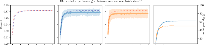
Batched RL update rules B-CL and B-MCL follow TRD and MRD respectively when the batch size () is large enough. As seen in Figure 4, it is clear that B-CL and B-MCL follow TRD and MRD respectively for large batch sizes (this can be seen from how the analytical solution is exactly at the center of the average reward curves of B-CL and B-MCL).
However, as soon we make the batch sizes smaller, the batched updates deviate from their analytical solutions (see sub-section 3.2). See supplementary Sec. A.1 for other environments. We also observe that B-MCL performs poorly compared to B-CL with smaller batch sizes, similar to observations made with non-batched RL experiments.
Convergence rate of MRD is TRD. As noted by Sandholm (2010), TRD and MRD can be rearranged in the form:
| (TRD) | (32) | ||||
| (MRD) | (33) |
being the update ”speed” and being bounded between 0 and 1.
The MRD speed is thus greater than the TRD speed.
Empirically, we observe that MRD converges faster than TRD, especially when the ’s are close to 0, as seen in the first column of Figure 1.
Whereas, when the ’s are near 1 there is no visible difference (as ). By extension, this also implies that MCL (for small ), B-MCL (for large batch size), and WVR (for large population) have convergence rates CL, B-CL, and VR respectively.
Population experiments with VR and WVR follow TRD and MRD respectively for large populations. It can be seen in Figure 3 that both VR and WVR follow TRD and MRD respectively when the population size is large. See supplementary Sec. A.2 for other environments. As soon as the population shrinks, VR and WVR start deviating from the analytical solution. Similar to the RL experiments, WVR performs poorly in comparison to VR for small population sizes.
Finally, from the discussions related to batched RL updates and
population experiments, we empirically validate Proposition 1 and Proposition 2.
6. Conclusions
With Propositions 1 and 2, we have demonstrated how RD is the underlying connection between Reinforcement Learning and Collective Decision-Making. Further, we have empirically validated this correspondence. This correspondence opens a bridge between these two fields, enabling the flow of ideas, new perspectives, and analogies for both. For example, it can be seen that Cross Learning, Maynard-Cross Learning, and, more generally, Reinforcement Learning take a single-agent perspective, where information from consecutive action samples/batches is accumulated into one centralized agent’s policy. On the other hand, and take a multi-agent perspective, where every individual implements simple local and decentralized rules, making independent decisions, which leads to an emergent collective policy.
Significance for RL. Similar to how we discovered a new RL update rule (i.e., Maynard-Cross Learning) from Swarm Intelligence, other ideas such as majority rule Valentini et al. (2016), and cross-inhibition Reina et al. (2017), can be used to create new update rules for Reinforcement Learning. Moreover, Swarm Intelligence algorithms are often inspired by nature, and thus require individuals to follow physics. This mandates practical constraints such as congestion Soma et al. (2023), communication, and finite size effects, which are generally ignored in Reinforcement Learning and population games. Comparing the performance of Reinforcement Learning agents with their equivalent swarm counterparts on such constraints is a direction for future work.
Significance for SI. The population-policy equivalence highlights how certain Swarm Intelligence methods are equivalent to single-agent Reinforcement Learning, demonstrating agency of the entire swarm as a single learning entity. Therefore, one could imagine that Multi-Agent Reinforcement Learning would similarly yield equivalent multi-swarm systems, where two or more coexisting swarms would compete/collaborate for resources (i.e., prisoners dilemma, hawk dove, etc). Further, ideas that empower Reinforcement Learning, could be ported to swarm intelligence and swarm robotics.
References
- (1)
- Auer et al. (2002) Peter Auer, Nicolò Cesa-Bianchi, and Paul Fischer. 2002. Finite-time Analysis of the Multiarmed Bandit Problem. Machine Learning 47 (05 2002), 235–256. https://doi.org/10.1023/A:1013689704352
- Bloembergen et al. (2015) Daan Bloembergen, Karl Tuyls, Daniel Hennes, and Michael Kaisers. 2015. Evolutionary Dynamics of Multi-Agent Learning: A Survey. Journal of Artificial Intelligence Research 53 (08 2015), 659–697. https://doi.org/10.1613/jair.4818
- Bonabeau et al. (1999) Eric Bonabeau, Marco Dorigo, and Guy Theraulaz. 1999. Swarm Intelligence: From Natural to Artificial Systems. Oxford University Press. https://doi.org/10.1093/oso/9780195131581.001.0001
- Castellano et al. (2009) Claudio Castellano, Santo Fortunato, and Vittorio Loreto. 2009. Statistical physics of social dynamics. Reviews of Modern Physics 81, 2 (May 2009), 591–646. https://doi.org/10.1103/revmodphys.81.591
- Cross (1973) John G. Cross. 1973. A Stochastic Learning Model of Economic Behavior. The Quarterly Journal of Economics 87, 2 (1973), 239–266. https://EconPapers.repec.org/RePEc:oup:qjecon:v:87:y:1973:i:2:p:239-266.
- Dorigo et al. (2006) Marco Dorigo, Mauro Birattari, and Thomas Stutzle. 2006. Ant colony optimization. IEEE Computational Intelligence Magazine 1, 4 (2006), 28–39. https://doi.org/10.1109/MCI.2006.329691
- Dorigo et al. (2021) Marco Dorigo, Guy Theraulaz, and Vito Trianni. 2021. Swarm Robotics: Past, Present, and Future [Point of View]. Proc. IEEE 109, 7 (2021), 1152–1165. https://doi.org/10.1109/JPROC.2021.3072740
- Hamann (2018) Heiko Hamann. 2018. Swarm Robotics: A Formal Approach. https://doi.org/10.1007/978-3-319-74528-2
- Kaufmann et al. (2023) Elia Kaufmann, Leonard Bauersfeld, Antonio Loquercio, Matthias Mueller, Vladlen Koltun, and Davide Scaramuzza. 2023. Champion-level drone racing using deep reinforcement learning. Nature 620 (08 2023), 982–987. https://doi.org/10.1038/s41586-023-06419-4
- Mnih et al. (2013) Volodymyr Mnih, Koray Kavukcuoglu, David Silver, Alex Graves, Ioannis Antonoglou, Daan Wierstra, and Martin A. Riedmiller. 2013. Playing Atari with Deep Reinforcement Learning. CoRR abs/1312.5602 (2013). arXiv:1312.5602 http://arxiv.org/abs/1312.5602
- Nowak (2006) Martin A. Nowak. 2006. Five Rules for the Evolution of Cooperation. Science 314, 5805 (2006), 1560–1563. https://doi.org/10.1126/science.1133755 arXiv:https://www.science.org/doi/pdf/10.1126/science.1133755
- Redner (2019) Sidney Redner. 2019. Reality-inspired voter models: A mini-review. Comptes Rendus. Physique 20, 4 (May 2019), 275–292. https://doi.org/10.1016/j.crhy.2019.05.004
- Reina et al. (2017) Andreagiovanni Reina, James A. R. Marshall, Vito Trianni, and Thomas Bose. 2017. Model of the best-of-N nest-site selection process in honeybees. Physical Review E 95, 5 (May 2017). https://doi.org/10.1103/physreve.95.052411
- Reina et al. (2024) Andreagiovanni Reina, Thierry Njougouo, Elio Tuci, and Timoteo Carletti. 2024. Speed-accuracy trade-offs in best-of- collective decision making through heterogeneous mean-field modeling. Phys. Rev. E 109 (May 2024), 054307. Issue 5. https://doi.org/10.1103/PhysRevE.109.054307
- Sandholm (2010) William H Sandholm. 2010. Population games and evolutionary dynamics. MIT press.
- Sandholm et al. (2008) William H. Sandholm, Emin Dokumacı, and Ratul Lahkar. 2008. The projection dynamic and the replicator dynamic. Games and Economic Behavior 64, 2 (2008), 666–683. https://doi.org/10.1016/j.geb.2008.02.003 Special Issue in Honor of Michael B. Maschler.
- Seo et al. (2024) Jaemin Seo, SangKyeun Kim, Azarakhsh Jalalvand, Rory Conlin, Andrew Rothstein, Joseph Abbate, Keith Erickson, Josiah Wai, Ricardo Shousha, and Egemen Kolemen. 2024. Avoiding fusion plasma tearing instability with deep reinforcement learning. Nature 626 (02 2024), 746–751. https://doi.org/10.1038/s41586-024-07024-9
- Smith (1982) John Maynard Smith. 1982. Evolution and the Theory of Games. Cambridge University Press, Cambridge, UK.
- Soma et al. (2023) Karthik Soma, Vivek Shankar Vardharajan, Heiko Hamann, and Giovanni Beltrame. 2023. Congestion and Scalability in Robot Swarms: A Study on Collective Decision Making. In 2023 International Symposium on Multi-Robot and Multi-Agent Systems (MRS). 199–206. https://doi.org/10.1109/MRS60187.2023.10416793
- Sutton and Barto (2018) Richard S Sutton and Andrew G Barto. 2018. Reinforcement learning: An introduction. MIT press.
- Taylor and Jonker (1978) Peter D. Taylor and Leo B. Jonker. 1978. Evolutionary stable strategies and game dynamics. Mathematical Biosciences 40, 1 (1978), 145–156. https://doi.org/10.1016/0025-5564(78)90077-9
- Valentini et al. (2016) Gabriele Valentini, Eliseo Ferrante, Heiko Hamann, and Marco Dorigo. 2016. Collective decision with 100 Kilobots: speed versus accuracy in binary discrimination problems. Autonomous Agents and Multi-Agent Systems 30, 3 (2016), 553–580. https://doi.org/10.1007/s10458-015-9323-3
- Valentini et al. (2014) Gabriele Valentini, Heiko Hamann, and Marco Dorigo. 2014. Self-organized collective decision making: the weighted voter model. In Proceedings of the 2014 International Conference on Autonomous Agents and Multi-Agent Systems (Paris, France) (AAMAS ’14). International Foundation for Autonomous Agents and Multiagent Systems, Richland, SC, 45–52.
- Visscher and Camazine (1999) P Kirk Visscher and Scott Camazine. 1999. Collective decisions and cognition in bees. Nature 397, 6718 (February 1999), 400. https://doi.org/10.1038/17047
- Williams (1992) Ronald J Williams. 1992. Simple Statistical Gradient-Following Algorithms for Connectionist Reinforcement Learning. , 229-256 pages.
- Xia et al. (2011) Haoxiang Xia, Huili Wang, and Zhaoguo Xuan. 2011. Opinion dynamics: A multidisciplinary review and perspective on future research. International Journal of Knowledge and Systems Science (IJKSS) 2, 4 (2011), 72–91.
Appendix A Supplementary material
A.1. Batched RL experiments


A.2. Population experiments


A.3. Hyperparametrs
In this section, we list out various hyperparameters used by RL and population experiments.
| Hyperparameter | value |
|---|---|
| Arms () | 10 |
| Learning rate () | |
| Epochs () | 100 |
| Variance ( | 1 |
| Runs () | |
| Weight factor () | 0.01 |
| Discretizing factor () | |
| final time () | = 100 |
| Hyperparameter | value |
|---|---|
| Arms () | 10 |
| Epochs () | 100 |
| Variance ( | 1 |
| Runs () | 100 |
| Batch size () | |
| Discretizing factor () | 1 |
| final time () | = 100 |
| Hyperparameter | value |
|---|---|
| Types/opinions () | 10 |
| Epochs () | 100 |
| Variance ( | 1 |
| Runs () | 100 |
| population size () | |
| Discretizing factor () | |
| final time () | = 100 |