Breathers in lattices with alternating strain-hardening and strain-softening interactions
Abstract
This work focuses on the study of time-periodic solutions, including breathers, in a nonlinear lattice consisting of elements whose contacts alternate between strain-hardening and strain-softening. The existence, stability, and bifurcation structure of such solutions, as well as the system dynamics in the presence of damping and driving are studied systematically. It is found that the linear resonant peaks in the system bend toward the frequency gap in the presence of nonlinearity. The time-periodic solutions that lie within the frequency gap compare well to Hamiltonian breathers if the damping and driving are small. In the Hamiltonian limit of the problem, we use a multiple scale analysis to derive a Nonlinear Schrödinger (NLS) equation to construct both acoustic and optical breathers. The latter compare very well with the numerically obtained breathers in the Hamiltonian limit.
I Introduction
Nonlinear lattices play a pivotal role in the modeling of a wide range of physical, biological, chemical, and electrical systems FPUreview ; pgk:2011 ; moti ; Morsch ; sievers . One of the prototypical examples, and most relevant for the present study, is the Fermi-Pasta-Ulam-Tsingou (FPUT) chain, which is simply a mass-spring system with nonlinear springs FPU55 . While the types of behavior that are possible in FPUT chains span a wide range, the structure we will focus on here is the so-called discrete breather, which is a solution that is localized in space and periodic in time. Discrete breathers (or just breathers) have been studied in a variety of physical systems, including, optical waveguide arrays and photorefractive crystals moti , micromechanical oscillator arrays sievers2 , Josephson-junction ladders alex ; alex2 , electrical lattices with nonlinear elements remoissenet , layered antiferromagnetic crystals lars3 ; lars4 , halide-bridged transition metal complexes swanson , dynamical models of the DNA double strand Peybi , Bose–Einstein condensates in optical lattices Morsch , and magnetic lattices moleron ; Mehrem2017 ; Marc2017 ; magBreathers ; Chong_2021 ; cantilevers among others.
One mechanical realization of an FPUT lattice that has attracted significant attention is the so-called granular chain, in which case the nonlinear interaction is described by a power-law with nonlinearity exponent . Granular chains consist of closely packed arrays of particles that interact elastically upon compression Nester2001 ; granularBook ; yuli_book ; Lindenberg_review ; gc_review ; sen08 . The contact force can be tuned to yield responses that range from near-linear to purely nonlinear, and the effective stiffness properties can also be easily changed by modifying the material, geometry, or contact angle of the elements in contact Nester2001 , although the stiffness will be of the strain-hardening type (implying an increase of elastic modulus with strain). Due to the strain-hardening nature of the granular chain, the monomer one (where all particles are identical) does not have genuine breather solutions JAMES201339 (although so-called dark breathers are possible dark ; dark2 ). Breathers are possible in granular chains with defects Theocharis2009 ; Nature11 or in mass-dimer chains Boechler2010 ; Theocharis10 ; hooge12 and have been studied in great detail.
More recently, strain-softening materials (implying a decrease of elastic modulus with strain) have been emerging as a new playground for the formation of nonlinear waves Deng2017 ; Raney , and the dynamics here will be distinct from their strain-hardening counterparts. For instance, rarefaction waves form in lattices with strain-softening interactions shock_trans_granular ; yasuda ; HEC_DSW instead of the classic solitary waves in the case of hardening lattices Nester2001 . Examples of lattices that have been argued to exhibit strain-softening interaction include tensegrity carpe , origami origami ; origami2 , stainless steel cylinders separated by polymer foams RarefactionNester , and hollow elliptical cylinders HEC_DSW . These strain-softening lattices can be modeled with FPUT type lattices with a power-law interaction with nonlinear exponent . Breathers in such strain-softening lattices are far less studied than their strain-hardening counterparts.
More novel still, to the best of our knowledge, is the study of breathers in lattices that feature both strain-hardening and strain-softening interactions, the focus of the present study. Such a lattice could be possible in an origami setting where each origami unit cell is tailored to have strain-hardening or strain-softening behavior. This is possible, in principle, given the highly tunable nature of origami by virtue of changes in crease-angle (see Bistable_origami for an example of an origami unit cell that can be tuned to exhibit both softening and hardening behavior, depending, e.g., on the folding angle for Tachi-Miura polyhedra origami ). Another possible realization is a chain of stainless steel cylinders in which only a subset of contacts is separated with a polymer foam in order to induce the strain-softening behavior.
The paper is structured as follows. The model equations and basic linear analysis of such a periodically alternating nonlinearity are given in Sec. II. Our main aim herein is to explore this model and especially its nonlinear time-periodic solutions. The numerical study of such breather (exponentially localized in space and periodic in time) waveforms of the damped-driven model (being more realistic for the potential experimental realization of such structures) is detailed in Sec. III. The ideal case of the Hamiltonian lattice is considered in Sec. IV, where the Nonlinear Schrödinger (NLS) equation is derived using a multiple-scale analysis in order to construct an analytical prediction of both acoustic and optical breathers. Section V concludes the paper and offers suggestions for future studies that build on the present one.
II Theoretical Setup
II.1 The model
A heterogeneous FPUT lattice with a power-law nonlinearity is given by Nester2001 ; FPU55
| (1) |
where the over-dot represents differentiation with respect to time , is the displacement of the -th particle from its equilibrium position, is a parameter accounting for the dissipation, and stands for the total number of particles in the chain. The bracket is defined via , and accounts for the (absence of force under potential) loss of contact between adjacent nodes. While general lattices with alternating stiffness will have mass (), equilibrium position (), and elastic properties () depend on the lattice location, we consider here a prototypical setting where we normalize them all to unity () for simplicity, except for the nonlinear exponent . This will allow us to elucidate differences that arise specifically from variations in stiffness as opposed to other variations. We consider nonlinear exponents that alternate in the following fashion
| (2) |
where and are parameters, i.e., we explore a form of a “nonlinearity dimer”. An important special case is that of (i.e., ), which corresponds to the case of the monomer granular crystal chain Nester2001 , in which case all particles are spheres. Other particle geometries can lead to other values of Nester2001 . In general, for the contact is strain-hardening. The practical interpretation of “strain-hardening” is that the “spring” connecting two nodes becomes harder to deform the larger the applied strain (this can be easily discerned by simply plotting the force relation ). Another special case is , which, as mentioned in the introduction, corresponds to tensegrity carpe , origami lattices origami ; origami2 , stainless steel cylinders separated by polymer foams RarefactionNester , and hollow elliptical cylinder lattices HEC_DSW . This is the “strain-softening” case, in which scenario the “spring” connecting two nodes becomes easier to deform the larger the applied strain. For non-constant (-dependent) nonlinear exponents of Eq. (2), the model [cf. Eq. (1)] that we propose considers softening and hardening behavior in an alternating fashion with and . Since the case of alternating stiffness type is what we are interested in here, we will mostly consider and . In this sense, our chain is, more concretely, a “stiffness dimer”, as opposed to the more commonly studied “mass-dimer” granularBook .
The chain [cf. Eq. (1)] is harmonically driven at the left boundary according to
| (3) |
with and being the amplitude and frequency of the (external) drive, and thus rendering the model a damped-driven one. At the right boundary of the chain, we assume a fixed wall which is modeled by .
It is worth mentioning that (the normalized version of) Eq. (1) with stems from the Euler-Lagrange equations:
| (4) |
with discrete Lagrangian density given by:
| (5) |
where
| (6) |
For this special case with , the Hamiltonian
| (7) |
is conserved when free boundary conditions are employed at the left and right ends of the chain, i.e., and , or in case the lattice is infinite in length, i.e., .
II.2 Linear Analysis
To obtain the dispersion relation and the eigenfrequency spectrum for the stiffness-dimer problem, we study in this section the linearized problem associated with Eq. (1). At first, if
| (8) |
then Eq. (1) reduces to
| (9) |
which, upon introducing and , i.e., even and odd displacements, respectively, can be written as
| (10a) | ||||
| (10b) | ||||
with solutions given by the Bloch ansatz:
| (11a) | ||||
| (11b) | ||||
Upon substituting Eqs. (11a)-(11b) into Eqs. (10a) (10b), we arrive at the following linear system for the amplitudes :
| (12) |
where therein. A non-trivial solution to the above system exists if the determinant of the matrix (containing the coefficients in Eq. (12)) is . This condition results in the following dispersion relation:
| (13) |
whose solutions read
| (14a) | ||||
| (14b) | ||||
and define the cut-off frequencies (at and ):
| (15a) | ||||
| (15b) | ||||
| (15c) | ||||
| (15d) | ||||
| (15e) | ||||
Here, it is relevant to note that the relevant frequencies are defined according to from the results of the dispersion relation. Moreover, the imaginary nature of the frequencies reflects the presence of loss, since entering the expressions of Eqs. (11a)-(11b) leads to a negative real part, reflecting the lossy part of the relevant exponential term. The top left panel of Fig. 1 shows the dispersion curves and the cut-off frequencies (see, also Eqs. (14a)-(14b)) as functions of the wavenumber . The existence of a frequency gap can be discerned from the figure.
In the case of homogeneous Dirichlet boundary conditions, i.e., , and for a finite domain, the above analytical solutions are no longer available, and the relevant eigenvalue problem is solved numerically (see, e.g., Ref. Stathis for details on the relevant calculation). Indeed, in the top right panel of Fig. 1, the frequencies obtained numerically for are shown with filled circles together with the cut-off frequencies (obtained analytically from Eqs. (15a)-(15e)) with dashed-dotted black lines. A perfect agreement can be discerned from this panel suggesting the consistency of our (linear) analysis. Example eigenvectors of the acoustic and optical bands are shown in the bottom left and right panels, respectively. It is interesting to observe that in the former (acoustic) case, the nodes bearing a softening nonlinearity are excited, while in the latter (optical) one, it is instead the hardening interaction nodes that are largely excited, while the softening ones are, for the most part, suppressed.
III Time-periodic solutions in the damped-driven chain


We now turn to the study of time-periodic solutions to the nonlinear problem with damping and driving. We will use primarily numerical computations for their study, but we discuss an analytical approximation in the next section using a reduction to the NLS equation in the Hamiltonian limit of the problem.
We compute time-periodic orbits, and their spectral stability, of Eq. (1) with period with high precision using a standard Newton-type procedure, see Appendix A for details. To investigate the dynamical stability of the obtained states, a Floquet analysis is used to compute the multipliers associated with the solutions. If a solution has all Floquet multipliers on or inside the unit circle, the solution is called (spectrally) stable. An instability that results from a multiplier on the (positive) real line is called a real (exponential in nature) instability. However, there can also be oscillatory instabilities, which correspond to complex-conjugate pairs of Floquet multipliers lying outside the unit circle (in the complex plane). In the bifurcation diagrams that are to follow in this paper, solid blue segments will correspond to stable parametric regions while the dashed-dotted red segments correspond to real unstable regions and green dashed-dotted segments correspond to oscillatorily unstable regions. The bifurcation diagrams are obtained using pseudo-arclength continuation as it is implemented in the software package AUTO Doedel . In all of the bifurcation diagrams that follow below, the monitored quantity that will be used is the average energy over one period defined as:
| (16) |
where
| (17) |
is the total energy, and
| (18) |
is the (discrete) energy density. Note that in Eq. (18) is given by Eq. (6).
For the numerical computations, we consider a chain with particles, and set , , and (unless explicitly stated otherwise). The drive amplitude and frequency will be used as continuation parameters. Let us start our presentation by considering Figs. 2-5, which correspond to frequency continuations. In particular, we consider the following cases: linear monomer chain () in Fig. 2, a strain-hardening monomer chain () in Fig. 3, a strain-softening monomer chain () in Fig. 4, and a dimer chain with alternating stiffness ( given by Eq. (2)) in Fig. 5. Figures 2-5 showcase the average energy [cf. Eq. (16)] as a function of the driving frequency . When , i.e., for the case corresponding to a linear lattice, it can be discerned from Fig. 2 that the resonant peaks match perfectly with the resonant frequencies of the respective linear problem shown with vertical dashed-dotted black lines (and solved numerically) in this case, as expected. Adding nonlinearity to the system will cause these linear resonant peaks to deform, or “bend”. For example, supposing that all contacts are strain-hardening, the resonant peaks will bend toward smaller frequencies, as shown in Fig. 3 where . If all contacts are strain-softening, the resonant peaks will bend toward larger frequencies as shown in Fig. 4 where . The observations in Figs. 3 and 4 are expected, and are inline with the established behavior for oscillators with hardening or softening nonlinearities Mook . In the bottom panels of Figs. 3 and 4, the resonant frequencies are depicted by vertical dashed-dotted lines (similar to Fig. 2) in order to ease the visualization of the bending of the resonant curves (to the left or right).
Having investigated the baseline cases of pure hardening and pure softening stiffness, we now turn to the aspect of alternating stiffness, i.e., Eq. (1) with nonlinearity exponents given by Eq. (2). The frequency continuation for this case is shown in Fig. 5 for . Notice the resonant peaks close to the top edge of the acoustic band and the bottom edge of the optical band all bend toward the gap due to the interplay of softening and hardening. This finding is shown in detail in the bottom panel of Fig. 5, which is a zoom of the top panel. Note that the eigenfrequency modes (shown with vertical dashed-dotted lines) help highlight this effect as well as the existence of a frequency gap. Note that in traditional mass-dimer lattices, resonant peaks from either the top of the acoustic band or the bottom of the optical band will bend into the frequency gap, but not both, like in the present case granularBook . The nature of the bending in the lattice with alternating stiffness can be understood in the small amplitude limit by inspection of the strain of the eigenvectors of the linear problem. In particular, within the acoustic band, the larger amplitude strains occur for odd indices, see the bottom left panel of Fig. 1. According to Eq. (2), the odd numbered interactions are of the softening type. Hence, one would expect softening-type dynamics, involving resonant peaks bending toward the right, as seen in Fig. 5. The situation in the optical band is reversed. The even numbered interactions have higher amplitude in the strain (see the bottom right panel of Fig. 1) indicating that hardening-type behavior should be observed, involving resonant peaks bending to the left, like in Fig. 5.
A discussion about the stability characteristics of the pertinent branches of Figs. 2-5 is now in order. In the linear lattice of Fig. 2, we observe that the entire branch is spectrally stable. In the nonlinear cases of Figs. 3-5, the branches are mostly stable, with exceptions occurring typically between two turning points. These segments, in line with what is known for classical oscillator systems Mook , are found to be unstable. For example, in Fig. 3 and for , the alternation of stable and unstable segments between turning points can be discerned. The instability in this case corresponds to an exponential one (and is shown with dashed-dotted red segments). A similar observation is found in Fig. 4 for drive frequencies . Interestingly, in some portions of the relevant branches, and in particular those of Figs. 3 and 5 (see the bottom panels therein), we find oscillatory instabilities. In these cases, the branches have been colored green to reflect this modified instability feature and the associated expected dynamics.
Besides the solutions that live on the main resonant curve shown in Fig. 5, there are also “isolas” of solutions, namely closed curves of solutions in the bifurcation diagram Isolas ; see Fig. 6 for example (and isola_strategy on how it was obtained). This isola lives entirely within the spectral gap. Periodic solutions with frequency that lie within a spectral gap are interesting since they are (necessarily) spatially localized. Such solutions are called nonlinear localized modes, or breathers Flach2007 . The case of damped-driven lattices where there is a driving source has attracted considerable attention in the present context. This is because of the intriguing interplay of localization due to the “defect” (i.e., the source) and that of the bulk breathers (or traveling waves) potentially available in the medium. This interplay can be used to produce hysteresis, metastability, resonances/antiresonances and related hallmarks of nonlinear dynamics that have been explored in a number of publications Nature11 ; hooge12 ; PhysRevE.92.063203 . It is interesting to highlight that there is a portion of the relevant isola branch that is found to be spectrally stable. The starting point of our subsequent study in this work will be to explore the time-periodic solutions of this system that have a frequency that lies in the spectral gap in the presence of damping and driving. Having examined those, we will subsequently turn to the case of the breathers in the Hamiltonian lattice.


We now fix the frequency (within the gap), and vary the amplitude of the drive, as shown in Fig. 7. We show the dependence of as a function of for a number of cases. The left and middle panels of Fig. 7 correspond to the hardening and softening cases, respectively, both with where the well-known hysteretic bifurcation diagram is obtained; see, e.g., Nature11 ; hooge12 . It should be noted in passing that the numerical results depicted in these panels are shown for amplitudes of the drive of up to and , respectively. The stability of the hysteretic bifurcation diagram is in line with earlier works Nature11 ; hooge12 . The fold bifurcations in the left panel of the figure occur at and . In the middle panel the bifurcation values are and . Notice, however, that there are distinctive features such as the short interval of oscillatory instability (for ) preceded by a very narrow segment (for ) of stable breathers in the middle panel of the softening case very near the bifurcation point. The right panel of the figure is a representative example for the alternating stiffness case (i.e., with nonlinearity exponents given by Eq. (2)) with lying in the frequency gap. The bifurcation curve (that is shown for drive amplitudes of up to ) becomes far more elaborate. It features a cascade of turning points, the first of which (i.e., at ) represents a fold bifurcation. Note that the labels (a)-(c) in the figure are connected with the numerical results of Fig. 8. Importantly, many of the numerous intermediate branches are found to be unstable through real instabilities, although the branch eventually features an oscillatory instability for sufficiently larger amplitude (as before). This additional complexity of the bifurcation diagram is introduced by means of the interplay between strain-softening and strain-hardening dynamics.


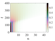
In Fig. 8 we show select examples of the dynamics of breather solutions (with no perturbation added on top of the respective initial conditions) for , which is in the spectral gap. Those solutions correspond to values of and are associated with the labels of the right panel of Fig. 7. The left column of Fig. 8 shows the strain profiles, i.e., where the insets depict the Floquet spectra. The solution in the top row is spectrally stable (and remains accordingly robust, although the energy quantity we measure oscillates due to the presence of damping and driving) whereas the ones in the middle and bottom are unstable. The one in the middle row is an exponentially unstable waveform since the instability is characterized by a real Floquet multiplier pair (with a dominant unstable mode of ), and the bottom one is oscillatory unstable corresponding to a complex multiplier quartet (with a dominant instability of ). The stability results are corroborated in the respective panels of the middle column of the figure which present the spatio-temporal evolution of the energy density [cf. Eq. (18)]. It can be seen in the middle panels of the second and third rows of the figure that after an unstable breather gets destroyed, a wavepacket is created which propagates with decreasing amplitude toward the bulk of the lattice. An additional part of the relevant energy is localized at the left edge of the computational domain and appears to localize forming a smaller amplitude breathing structure therein. At longer times, these structures gradually asymptote to the stable solution of the top left panel of the figure. This finding can be further explored by looking at the right column of the figure. In particular, we present the total energy of Eq. (17) as a function of time in the respective cases. In the top right panel of the figure, the total energy of the stable solution oscillates, as discussed above, but maintains a nearly constant average of about 0.245 for periods. On the other hand, in the middle and bottom panels, the energy experiences large deviations, highlighting the onset of the instability. Both unstable solutions eventually approach the stable one shown in the top row. This can be seen in the energy plots, where the average energy approaches 0.245 at for the unstable breather with label (b) and at for the unstable breather with label (c).
In all the numerical results that we have presented so far, was considered in Eq. (1). Next, we will study the effect of varying the dissipation parameter , where we gradually decrease it in order to approach the Hamiltonian limit. Moreover, this study will be beneficial while connecting the respective results presented herein with the ones of Sec. IV for . Let us start our discussion by considering Fig. 9 which corresponds to the value of driving frequency of being itself the cut-off frequency of the bottom optical edge of the optical band (see the right panel of Fig. 1). From the left to the right panels of the figure, the dependence of is shown as a function of for , , and , respectively. We mention in passing the existence of a cascade of turning points in the panels, with the first four happening (as we trace the bifurcation curve from with increasing arclength) at (left), (middle), and (right). A movie illustrating how the solution profile changes as one moves along the bifurcation curve of the right panel is included in the supplement.
As the value of the dissipation parameter decreases, when , Eq. (1) approaches its Hamiltonian sibling, i.e., when . Indeed, the solutions at the turning points in the right panel with (and ), aside from the lowest one introduced by the drive and vanishing in this limit, are expected to be proximal to Hamiltonian breathers, since they are large amplitude (energy) states that exist in the lattice with nearly zero drive and zero damping. Recall that in the above diagrams we have fixed the frequency at the lower optical band edge. Bifurcation diagrams for frequencies deeper in the gap generally follow the same trend, namely that the turning points move toward smaller drive amplitude as the damping is decreased. However, the overall bifurcation structure is more intricate, as we explore next. Moreover, we would like to report an intriguing feature that happens at the turning points of the above mentioned bifurcation diagrams. As we approach a turning point, two eigenvalues are moving (one from the first and the other one from the fourth quadrant inside the unit circle) toward the real axis, until they collide exactly at the turning point, and past that, a pair of real multipliers emerges. We note that for the Hamiltonian problem at hand, such a collision happens at but for the present damped-driven problem, the collisions happen slightly inside the unit circle. More concretely, in the middle panel of Fig. 9, the eigenvalues at the first turning point (i.e., ) are and . Interestingly and in line with similar earlier observations in jesus , they satisfy the relation which for the Hamiltonian case, i.e., , it gives . Indeed, we have and . We further checked the relation at the other turning points and cases in (right panel of the figure), and it holds indeed. It should also be noted that this implies that the stability change does not arise at the turning point but only nearby, given that the collision happens inside of the unit circle, and hence further parametric tuning is needed for one of the (now real) multipliers to cross the point.


The connection between the damped-driven and Hamiltonian breathers is explored in Fig. 10. We chose a frequency that is in the gap, namely , and a small damping parameter . At this frequency, the amplitude continuation (analogous to the one shown in Fig. 9) yields a more intricate bifurcation diagram (see the top left and middle panels in the figure). It is expected that a solution lying at a turning point with small driving amplitude (see the orange square marker in the inset of the top middle panel) will be proximal to an associated Hamiltonian breather, i.e., an intrinsic localized mode of Eq. (1) with . The velocity profile of the damped-driven breather (corresponding to the orange square maker of the top middle panel) is shown in blue in the top right panel of the figure. The solution itself compares fairly well with the Hamiltonian breather, which is shown in red.


In order to construct Hamiltonian breathers of Eq. (1) numerically, we consider a lattice with beads and employ zero Dirichlet and free boundary conditions at the endpoints of the chain, respectively, i.e., and . The larger lattice size was needed in order to minimize the effect of the boundary conditions (since the strain of the breather solution is nearly zero at the boundaries for large lattices). The initial guess to our solvers was provided by the associated linear mode at the bottom edge of the optical band of the Hamiltonian problem (i.e., when ). The Hamiltonian breathers found in this way are centered at the middle of the lattice. Thus, in order to compare the obtained breather to the damped-driven one (which is localized at the source of the drive, namely the left boundary) we translate the Hamiltonian breather so that the largest amplitude is on the boundary. This is how the comparison shown the the top right panel of Fig. 10 was made, showcasing the proximity between the two.
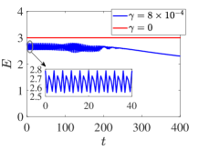
The insets of the top right panel of Fig. 10 indicate that the breathers of the damped-driven model and its Hamiltonian version are both exponentially unstable (with dominant unstable modes of and , respectively), in addition to being extremely proximal to each other profile-wise. It should be reminded here that the difference in the density of Floquet multipliers populating the unit circle between the damped-driven (left) and Hamiltonian (right) insets stems from the different corresponding size lattices. This stability analysis is corroborated in the bottom left and middle panels of Fig. 10 where the spatio-temporal evolution of the energy density of (randomly) perturbed breathers is shown therein. It can be discerned from the figure that the instability in the damped-driven case manifests itself slightly earlier than in the Hamiltonian one, in line with our observation of the slightly larger (instability) growth rate. Moreover, the bottom right panel showcases the total energy as a function of time in both cases. Although the (averaged) energy in the damped-driven case (shown in blue therein) is bounded, it starts deviating at from its original value signaling the onset of the instability. On the other hand, and as per the Hamiltonian nature of the breather, the energy is conserved (and shown in red), i.e., in this case, the energy is not a suitable diagnostic for discerning the instability, yet its conservation is indicative of the accuracy of the numerical simulation. On the other hand, if we probe the total energy of the first 5 sites, one can see that this local energy portion starts deviating around from its initial (unstable equilibrium) value, thus signaling the onset of the instability, in line with the dynamical evolution of the left panel of Fig. 11. In both cases, over suitably long times, we observe that the resulting dynamical outcome is rather similar although the Hamiltonian system features longer-lived (and total-energy-preserving) dispersive radiation. In the dissipative case, the relevant energy appears to decay away due to the damped nature of the lattice bulk. While here we compared a Hamiltonian breather with damped-driven breather located at a single turning point in the bifurcation diagram, there is in fact a zoo of such solutions (one at each turning point in the bifurcation diagram), see the middle and right panels of Fig. 11. A more systematic study of all the relevant waveforms may be an interesting topic for further study.


IV NLS approximation of the Hamiltonian breathers
We have just shown that when the damping is small, the Hamiltonian breathers are close to breather solutions of the damped-driven lattice. In the former case we can analytically approximate breather solutions by deriving an NLS equation to describe slow modulations in time and space of an underlying carrier wave. The NLS equation has an exact soliton solution, and thus one can obtain an analytical approximation in this way. The derivation of the NLS equation we present is similar to the one performed in Huang2 for a mass-dimer, but differs in a few key ways, which is why we include the derivation here.
At first, we re-write the equation of motion of Eq. (1) with in terms of even () and odd () particles as
| (19a) | ||||
| (19b) | ||||
Recall that , while above and in what follows. Upon assuming and , Eqs. (19a)-(19b) reduce into
| (20a) | ||||
| (20b) | ||||
where () is defined by
with coefficients , , , and .
Next, solutions in the form of fast oscillating yet small in amplitude patterns modulated by envelopes (that vary slowly in space and time) are sought by the following multiple scale Ansätze:
| (21a) | ||||
| (21b) | ||||
where as well as , , and . Note that , and also and with the bar standing for complex conjugation. Based on Eqs. (21a)-(21b), we also have that
| (22a) | ||||
| (22b) | ||||
together with the following Taylor expansions:
| (23a) | ||||
| (23b) | ||||
Since we are interested in standing breather solutions, we now set and hence . Thus, the two possible frequencies from which we perturb are , corresponding to the the lower optical cut-off frequency, and , corresponding to the upper acoustic cut-off frequency.
We now plug Eqs. (21a)-(21b) into Eqs. (20a)-(20b), and collect coefficients of each term. In particular, Eq. (20a) (after suppressing the dependence for ) gives, up to the first two orders:
| (24a) | ||||
| (24b) | ||||
| (24c) | ||||
| (24d) | ||||
| (24e) | ||||
Similarly, Eq. (20b) gives:
| (25a) | ||||
| (25b) | ||||
| (25c) | ||||
| (25d) | ||||
| (25e) | ||||
From Eqs. (24b) and (25b), we can express the underlying system as with
| (26) |
which has a non-trivial solution provided that has a vanishing determinant. It should be noted in passing that the matrix is the same as the one of Eq. (12) with . The vanishing determinant of yields the dispersion relation
| (27) |
where the “” subscript corresponds to the lower cut-off of the optical band, and the “” subscript corresponds to the upper cut-off of the acoustic band. In addition, from Eq. (25b) (same argument can be deduced by using Eq. (24b)), we obtain:
| (28) |
based on the dispersion relation.
Upon utilizing Eqs. (24a) and (25a), Eqs. (24d) and (25d) yield:
| (29a) | ||||
which (with the aid of Eq. (28)) can be cast into
| (30) |
Since the matrix is singular (note that the superscripts emanate from , it follows that (where stands for its transpose) has a non-trivial one-dimensional kernel. Indeed, it is then a direct calculation to identify:
| (31) |
such that (upon using Eq. (27) too). In addition, and upon considering the Fredholm alternative for Eq. (30), we can show that the latter indeed has a solution if and only if the right hand side of Eq. (30) is orthogonal to the co-kernel of (that is, the kernel of ).
We now consider Eqs. (24e) and (25e). With the aid of Eqs. (27) and (28), we arrive at
| (32) |
Next we consider the equations, and in particular Eq. (24c) which is solved with respect to (the exact same solution is obtained from Eq. (25c)), thus yielding:
| (33) |
Next, we focus on the equations for (shown in the Appendix B) from which we will obtain an equation for that depends on and its (complex) conjugate. Upon utilizing Eqs. (24a), (25a), and (28), one can find the component. Then, if one plugs the expression for [cf. Eq. (33)] as well as into the equation for , and solves subsequently with respect to , one obtains:
| (34) |
Note that Eq. (34) can be integrated once with respect to , thus yielding
| (35) |
where is an arbitrary function of . Considering our interest in structures that asymptotically vanish at we set . It should be noted in passing that when (i.e., the monomer case), the prefactor is exactly the same as the one in granularBook (see, Eq. (A19) therein).
Finally, we focus on the equations for both and , where we will find the NLS equation. At first, we express in terms of :
which emanates from the (singular) system of Eq. (30). Next, we utilize Eqs. (24a), (25a), (28), (32), and Eq. (33). This way, we obtain the following system at :
| (36a) | ||||
| (36b) | ||||
which can be re-cast into
| (37) |
where the residual vector is given by
| (38) |
However, and due to the Fredholm alternative, the vector is orthogonal to , i.e., , thus this compatibility condition yields the modulation equation for , i.e., the standard NLS equation:
| (39) |
where
| (40a) | ||||
| (40b) | ||||
In the focusing case, i.e., when , the bright-soliton solution of the NLS [cf. Eq. (39)] is given by
| (41) |
where is an arbitrary constant that has the opposite sign of . For simplicity sake, we set . With the parameter values used throughout the manuscript, i.e., and , we have that and in this case . We also have that and in this case . Note that and , namely the NLS is focusing at both the top of the acoustic band and the bottom of the optical band. This is in contrast to classical mass-dimer chains, where only one edge typically leads to a focusing NLS equation granularBook . Keeping the two lowest order terms of Eqs. (21a) with the soliton solution for and the subsequent relation Eq. (35) to compute , we can finally write down an approximate breather solution. For the breather near the top edge of the acoustic band , we have
| (42) | |||||
| (43) |
and by virtue of Eqs. (28) and (25a), a similar expression for is obtained. This is a spatially localized solution with temporal frequency , which is slightly above the edge of the acoustic band that sits on top of a stationary kink background. The acoustic breather would be out-of-phase if one subtracts off the stationary kink background (due to Eq. (28)). For the breather near the bottom edge of the optical band , we have
| (44) |
A similar expression for is obtained. Note that, to leading order, we have that . This implies the optical breather is in-phase. The frequency of the oscillation is , which is slightly below the edge of the optical band .


Both the acoustic and optical breathers have essentially the same structure, with the major difference being the sign of the leading order kink background. These approximate breather solutions compare well to those computed numerically for small values of , see Fig. 12 for example. Note that these formulas predict that the breathers will become larger, and more localized, as the frequency goes deeper into the spectral gap (and no bifurcation is predicted). However, the approximation becomes less accurate as frequencies deviate from the spectral edges, since is becoming larger. In particular, breathers of the full lattice system are expected to terminate or experience other bifurcations, like those reported in dark . Finally, we conclude our discussion here by mentioning the connection between the approximate breathers and the ones computed numerically for the dissipative problem with and (see, the profile in the top right panel of Fig. 10). The relevant comparison is shown in Fig. 13 where a proximity between the two profiles is observed. This confirms the fact that as we approach the point of small dissipation and drive amplitudes, the waveforms of interest essentially are the ones bifurcating from the Hamiltonian limit that our above NLS multiple scales analysis allows us to accurately approximate.

V Conclusions and Future Challenges
We have proposed a new model that involves a mixture of strain-hardening and strain-softening interactions, and studied time-periodic and breather solutions therein. The nonlinear resonant peaks of the damped-driven system bend toward the frequency gap, but they do so in different ways in the case of the acoustic and optical gaps herein. The high-energy states that enter the frequency gap are spatially localized (e.g. breathers) and are found to compare well to Hamiltonian breathers when the damping and drive amplitude are small. The complex bifurcation diagrams associated with the damped-driven chain has been obtained and their fold bifurcations, as well as the ones leading to oscillatory instabilities have been elucidated. The dynamics of the unstable waveforms have also been probed, and it has been observed that they repartition the energy, possibly through weaker localization at the boundary and dispersion of wavepackets towards the bulk of the chain. In the Hamiltonian lattice limit, we derived an NLS equation and from there, we were able to construct approximate acoustic and optical breathers, both of which agree well with numerically computed breathers in the vicinity of the corresponding band edges.
While breathers are fundamental in the study of nonlinear lattices, other structures, such as solitary waves or dispersive shocks merit further exploration in lattices with alternating stiffness. Some indications towards the potential relevance of such structures have also appeared herein in settings where the energy was shown to somewhat coherently propagate through such lattices. It would be interesting to parallel relevant studies to the well-established picture of resonances and anti-resonances in standard granular (mass) dimers staros1 . Similarly to the latter setting JKdimer , it is reasonable to expect that such dimers can be implemented also in the present setting. Moreover, the study of granular chains with nonlinearity exponents close to unity is of extensive mathematical interest, as illustrated by the work of pelingj and the numerous ones that followed along the related direction of the continuum log-KdV model. Although we did not pursue such a connection here, it would be a natural one to also consider in the setting proposed herein. Extensions to higher spatial dimension are also worthy of additional exploration, especially since the existence of breathers in the latter setting is far less explored in the granular case; see, e.g., Chong_2021 for a recent discussion. Finally, the proposed model seems well within current experimental capabilities, and such studies would not only test the viability of breather solutions in such lattices, but may also offer insights for potential applications of lattices with alternating stiffness, such as in shock absorption or energy harvesting. Such studies are currently in progress and will be reported in future publications.
Acknowledgements.
This material is based upon work supported by the Research, Scholarly & Creative Activities Program awarded by the Cal Poly division of Research, Economic Development & Graduate Education (MML, EGC, and SX) and the US National Science Foundation under Grant Nos. DMS-2107945 (CC) and DMS-1809074 (PGK). EGC expresses his gratitude to A. Vainchtein (University of Pittsburgh) for discussions related to the derivation of the NLS.Appendix A Newton’s method and spectral stability
We first compute time-periodic orbits of Eq. (1) with period with high precision by finding roots of the map , where is the solution of Eq. (1) at time with initial condition . Roots of this map (and hence time-periodic solutions of Eq. (1)) are found via Newton iterations. This requires the Jacobian of , which is of the form , where is the identity matrix, is the solution to the variational equations with initial condition and is the Jacobian of the equations of motion evaluated at a given state vector of the form of where . Note that the solution frequency and drive frequency are both by construction. To investigate the dynamical stability of the obtained states, a Floquet analysis is used to compute the multipliers associated with the solutions. The Floquet multipliers for a solution are obtained by computing the eigenvalues of the monodromy matrix (which is upon convergence of the Newton scheme). If a solution has all Floquet multipliers within or on the unit circle, the solution is called (spectrally) stable. An instability that results from a multiplier on the (positive) real line is called a real (exponential in nature) instability. However, there can also be oscillatory instabilities, which correspond to complex-conjugate pairs of Floquet multipliers lying outside the unit circle (in the complex plane).
Appendix B The equations
In this Appendix, we present the equations for the variables and ( and ). We obtain these equations by utilizing together with Eq. (28). This way, the equations for the lower cut-off of the optical band read
| (45a) | ||||
| (45b) | ||||
As it was already mentioned in the text, we solve Eq. (45b) with respect to first, and plug the resulting expression in Eq. (45a) afterwards. Then, and upon using Eq. (33) and its derivative (to eliminate the terms), we thus arrive at Eq. (34) for the component.
References
- [1] G. Gallavotti. The Fermi–Pasta–Ulam Problem: A Status Report. Springer-Verlag, Berlin, Germany, 2008.
- [2] P. G. Kevrekidis. Non-linear waves in lattices: past, present, future. IMA J. Appl. Math., 76:389–423, 2011.
- [3] F. Lederer, G. I. Stegeman, D. N. Christodoulides, G. Assanto, M. Segev, and Y. Silberberg. Discrete solitons in optics. Phys. Rep., 463:1, 2008.
- [4] O. Morsch and M. Oberthaler. Dynamics of Bose–Einstein condensates in optical lattices. Rev. Mod. Phys., 78:179, 2006.
- [5] M. Sato, B. E. Hubbard, and A. J. Sievers. Colloquium: Nonlinear energy localization and its manipulation in micromechanical oscillator arrays. Rev. Mod. Phys., 78:137, 2006.
- [6] E. Fermi, J. Pasta, and S. Ulam. Studies of Nonlinear Problems. I. Tech. Rep., (Los Alamos National Laboratory, Los Alamos, NM, USA):LA–1940, 1955.
- [7] M. Sato, B. E. Hubbard, L. Q. English, A. J. Sievers, B. Ilic, D. A. Czaplewski, and H. G. Craighead. Study of intrinsic localized vibrational modes in micromechanical oscillator arrays. Chaos: An Interdisciplinary Journal of Nonlinear Science, 13(2):702–715, 2003.
- [8] P. Binder, D. Abraimov, A. V. Ustinov, S. Flach, and Y. Zolotaryuk. Observation of breathers in Josephson ladders. Phys. Rev. Lett., 84:745, 2000.
- [9] E. Trías, J. J. Mazo, and T. P. Orlando. Discrete breathers in nonlinear lattices: Experimental detection in a Josephson array. Phys. Rev. Lett., 84:741, 2000.
- [10] M. Remoissenet. Waves Called Solitons. Springer-Verlag, Berlin, 1999.
- [11] L. Q. English, M. Sato, and A. J. Sievers. Modulational instability of nonlinear spin waves in easy-axis antiferromagnetic chains. ii. influence of sample shape on intrinsic localized modes and dynamic spin defects. Phys. Rev. B, 67:024403, 2003.
- [12] U. T. Schwarz, L. Q. English, and A. J. Sievers. Experimental generation and observation of intrinsic localized spin wave modes in an antiferromagnet. Phys. Rev. Lett., 83:223, 1999.
- [13] B. I. Swanson, J. A. Brozik, S. P. Love, G. F. Strouse, A. P. Shreve, A. R. Bishop, W.-Z. Wang, and M. I. Salkola. Observation of intrinsically localized modes in a discrete low-dimensional material. Phys. Rev. Lett., 82:3288, 1999.
- [14] M. Peyrard. Nonlinear dynamics and statistical physics of DNA. Nonlinearity, 17:R1, 2004.
- [15] M. Molerón, A. Leonard, and C. Daraio. Solitary waves in a chain of repelling magnets. Journal of Applied Physics, 115(18):184901, 2014.
- [16] A. Mehrem, N. Jiménez, L. J. Salmerón-Contreras, X. García-Andrés, L. M. García-Raffi, R. Picó, and V. J. Sánchez-Morcillo. Nonlinear dispersive waves in repulsive lattices. Phys. Rev. E, 96:012208, 2017.
- [17] M. Serra-Garcia, M. Molerón, and C. Daraio. Tunable, synchronized frequency down-conversion in magnetic lattices with defects. Phil. Trans. Roy. Soc. A: Math. Phys. Eng. Sci., 376(2127):20170137, 2018.
- [18] M. Molerón, C. Chong, A. J. Martínez, M. A. Porter, P. G. Kevrekidis, and C. Daraio. Nonlinear excitations in magnetic lattices with long-range interactions. New Journal of Physics, 21:063032, 2019.
- [19] C. Christopher, Y. Wang, D. Maréchal, E. G. Charalampidis, M. Molerón, A. J. Martínez, M. A. Porter, P. G. Kevrekidis, and C. Daraio. Nonlinear localized modes in two-dimensional hexagonally-packed magnetic lattices. New Journal of Physics, 23(4):043008, apr 2021.
- [20] C. Chong, A. Foehr, E. G. Charalampidis, P. G. Kevrekidis, and C. Daraio. Breathers and other time-periodic solutions in an array of cantilevers decorated with magnets. Mathematics in Engineering, 1:489–507, 2019.
- [21] V.F. Nesterenko. Dynamics of Heterogeneous Materials. Springer-Verlag, New York, 2001.
- [22] C. Chong and P. G. Kevrekidis. Coherent Structures in Granular Crystals: From Experiment and Modelling to Computation and Mathematical Analysis. Springer, New York, 2018.
- [23] Yu. Starosvetsky, K.R. Jayaprakash, M. Arif Hasan, and A.F. Vakakis. Dynamics and Acoustics of Ordered Granular Media. World Scientific, Singapore, 2017.
- [24] A. Rosas and K. Lindenberg. Pulse propagation in granular chains. Physics Reports, 735:1 – 37, 2018.
- [25] C. Chong, Mason A. Porter, P. G. Kevrekidis, and C. Daraio. Nonlinear coherent structures in granular crystals. J. Phys.: Condens. Matter, 29:413003, 2017.
- [26] S. Sen, J. Hong, J. Bang, E. Avalos, and R. Doney. Solitary waves in the granular chain. Phys. Rep., 462:21, 2008.
- [27] G. James, P. G. Kevrekidis, and J. Cuevas. Breathers in oscillator chains with hertzian interactions. Physica D: Nonlinear Phenomena, 251:39–59, 2013.
- [28] C. Chong, P. G. Kevrekidis, G. Theocharis, and Chiara Daraio. Dark breathers in granular crystals. Phys. Rev. E, 87:042202, 2013.
- [29] C. Chong, F. Li, J. Yang, M. O. Williams, I. G. Kevrekidis, P. G. Kevrekidis, and C. Daraio. Damped-driven granular chains: An ideal playground for dark breathers and multibreathers. Phys. Rev. E, 89:032924, 2014.
- [30] G. Theocharis, M. Kavousanakis, P. G. Kevrekidis, C. Daraio, M. A. Porter, and I. G. Kevrekidis. Localized breathing modes in granular crystals with defects. Phys. Rev. E, 80:066601, 2009.
- [31] N. Boechler, G. Theocharis, and C. Daraio. Bifurcation-based acoustic switching and rectification. Nat. Mater., 10(9):665–668, 2011.
- [32] N. Boechler, G. Theocharis, S. Job, P. G. Kevrekidis, M. A. Porter, and C. Daraio. Discrete breathers in one-dimensional diatomic granular crystals. Phys. Rev. Lett., 104:244302, 2010.
- [33] G. Theocharis, N. Boechler, P. G. Kevrekidis, S. Job, M. A. Porter, and C. Daraio. Intrinsic energy localization through discrete gap breathers in one-dimensional diatomic granular crystals. Phys. Rev. E, 82:056604, 2010.
- [34] C. Hoogeboom, Y. Man, N. Boechler, G. Theocharis, P. G. Kevrekidis, I. G. Kevrekidis, and C. Daraio. Hysteresis loops and multi-stability: From periodic orbits to chaotic dynamics (and back) in diatomic granular crystals. Euro. Phys. Lett., 101:44003, 2013.
- [35] B. Deng, J. R. Raney, V. Tournat, and K. Bertoldi. Elastic vector solitons in soft architected materials. Phys. Rev. Lett., 118:204102, 2017.
- [36] J. Raney, N. Nadkarni, C. Daraio, D. M. Kochmann, J. A. Lewis, and K. Bertoldi. Stable propagation of mechanical signals in soft media using stored elastic energy. Proceedings of the National Academy of Sciences, 2016.
- [37] E. B. Herbold and V. F. Nesterenko. Shock wave structure in a strongly nonlinear lattice with viscous dissipation. Phys. Rev. E, 75:021304, 2007.
- [38] H. Yasuda, C. Chong, J. Yang, and P. G. Kevrekidis. Emergence of dispersive shocks and rarefaction waves in power-law contact models. Phys. Rev. E, 95:062216, 2017.
- [39] H. Kim, E. Kim, C. Chong, P. G. Kevrekidis, and J. Yang. Demonstration of dispersive rarefaction shocks in hollow elliptical cylinder chains. Phys. Rev. Lett., 120:194101, 2018.
- [40] F. Fraternali, G. Carpentieri, A. Amendola, R. E. Skelton, and V. F. Nesterenko. Multiscale tunability of solitary wave dynamics in tensegrity metamaterials. Applied Physics Letters, 105(20):201903, 2014.
- [41] H. Yasuda, C. Chong, E. G. Charalampidis, P. G. Kevrekidis, and J. Yang. Formation of rarefaction waves in origami-based metamaterials. Phys. Rev. E, 93:043004, 2016.
- [42] H. Yasuda, Y. Miyazawa, E. G. Charalampidis, C. Chong, P. G. Kevrekidis, and J. Yang. Origami-based impact mitigation via rarefaction solitary wave creation. Science Advances, 5:eaau2835, 2019.
- [43] E. B. Herbold and V. F. Nesterenko. Propagation of rarefaction pulses in discrete materials with strain-softening behavior. Phys. Rev. Lett., 110:144101, 2013.
- [44] H. Yasuda and J. Yang. Reentrant origami-based metamaterials with negative Poisson’s ratio and bistability. Phys. Rev. Lett., 114:185502, 2015.
- [45] E. G. Charalampidis, F. Li, C. Chong, J. Yang, and P. G. Kevrekidis. Time-periodic solutions of driven-damped trimer granular crystals. Math. Probl. in Eng., 2015:830978, 2015.
- [46] E. Doedel and L. S. Tuckerman. Numerical Methods for Bifurcation Problems and Large-Scale Dynamical Systems. Springer-Verlag, Heidelberg, Germany, 2000.
- [47] A. H. Nayfeh and D. T. Mook. Nonlinear Oscillations. Wiley and Sons, Weihheim, Germany, 2004.
- [48] M. Beck, J. Knobloch, D. J. B. Lloyd, B. Sandstede, and T. Wagenknecht. Snakes, ladders, and isolas of localized patterns. SIAM Journal on Mathematical Analysis, 41(3):936–972, 2009.
- [49] This isola was obtained by performing a frequency continuation in AUTO. The initial seed that was fed to the solver was extracted from the branch shown in the rightmost panel of Fig. 7 for (and ).
- [50] S. Flach and A. Gorbach. Discrete breathers: advances in theory and applications. Phys. Rep., 467:1, 2008.
- [51] D. Pozharskiy, Y. Zhang, M. O. Williams, D. M. McFarland, P. G. Kevrekidis, A. F. Vakakis, and I. G. Kevrekidis. Nonlinear resonances and antiresonances of a forced sonic vacuum. Phys. Rev. E, 92:063203, 2015.
- [52] Anna Vainchtein, Jesús Cuevas-Maraver, Panayotis G. Kevrekidis, and Haitao Xu. Stability of traveling waves in a driven Frenkel–Kontorova model. Communications in Nonlinear Science and Numerical Simulation, 85:105236, 2020.
- [53] G. Huang and B. Hu. Asymmetric gap soliton modes in diatomic lattices with cubic and quartic nonlinearity. Phys. Rev. B, 57:5746, 1998.
- [54] K. R. Jayaprakash, Y. Starosvetsky, and A. F. Vakakis. New family of solitary waves in granular dimer chains with no precompression. Phys. Rev. E, 83:036606, 2011.
- [55] E. Kim, R. Chaunsali, H. Xu, J. Castillo, J. Yang, P. G. Kevrekidis, and A. F. Vakakis. Nonlinear low-to-high frequency energy cascades in diatomic granular crystals. Phys. Rev. E, 92:062201, 2015.
- [56] G. James and D. Pelinovsky. Gaussian solitary waves and compactons in Fermi–Pasta–Ulam lattices with Hertzian potentials. P. Roy. Soc. A-Math-Phy., 470(2165), 2014.