BP3M: Bayesian Positions, Parallaxes, and Proper Motions derived from the Hubble Space Telescope and Gaia data
Abstract
We present a hierarchical Bayesian pipeline, BP3M, that measures positions, parallaxes, and proper motions (PMs) for cross-matched sources between Hubble Space Telescope (HST) images and Gaia – even for sparse fields ( per image) – expanding from the recent GaiaHub tool. This technique uses Gaia-measured astrometry as priors to predict the locations of sources in HST images, and is therefore able to put the HST images onto a global reference frame without the use of background galaxies/QSOs. Testing our publicly-available code in the Fornax and Draco dSphs, we measure accurate PMs that are a median of 8-13 times more precise than Gaia DR3 alone for . We are able to explore the effect of observation strategies on BP3M astrometry using synthetic data, finding an optimal strategy to improve parallax and position precision at no cost to the PM uncertainty. Using 1619 HST images in the sparse COSMOS field (median 9 Gaia sources per HST image), we measure BP3M PMs for 2640 unique sources in the range, 25% of which have no Gaia PMs; the median BP3M PM uncertainty for sources is compared to from Gaia, while the median BP3M PM uncertainty for sources without Gaia-measured PMs () is . The statistics that underpin the BP3M pipeline are a generalized way of combining position measurements from different images, epochs, and telescopes, which allows information to be shared between surveys and archives to achieve higher astrometric precision than that from each catalog alone.
1 Introduction
High precision proper motions (PM) of individual stars have dramatically increased our understanding of kinematics in the Local Group. In particular, the Hubble Space Telescope (HST) has a rich history of providing the precise astrometry needed to make accurate motion measurements. This is thanks to detailed work over the last few decades to characterize and correct HST geometric distortions, describe point spread functions (PSFs), and define best practices for mapping images onto one another (e.g. Anderson & King, 2004, 2006; Anderson, 2007; Bellini & Bedin, 2009; Bellini et al., 2011). As a result, the PMs measured from multi-epoch HST imaging have been used to study key astronomical questions, such as the relative motion of the Milky Way (MW) and M31 (Sohn et al., 2012; van der Marel et al., 2012), the mass of the MW (Sohn et al., 2018), and MW stellar halo kinematic measurements in individual fields (Cunningham et al., 2019b).
More recently, the Gaia mission (Gaia Collaboration et al., 2018) has facilitated substantial leaps in Local Group science by providing full astrometric solutions for millions of stars. In the MW, these results include the identification of our most massive merger, the Gaia-Sausage-Enceladus (e.g Helmi et al., 2018; Belokurov et al., 2018; Mackereth et al., 2019), detailed inventories of the progenitors that built the MW (e.g. Naidu et al., 2020), and nearly-complete catalogs of the motions of nearby globular clusters (Vasiliev & Baumgardt, 2021).
While both of these telescopes have and will continue to fundamentally alter our knowledge about the local universe, they both have limitations. In HST’s case, the small field of view and relatively long observation times mean that only a small portion of the sky has been observed at multiple epochs with significant time baselines. For Gaia, their all-sky catalog necessarily does not see as faint as a standard HST observation, and the precision of their astrometric solutions decreases fairly significantly for their faintest magnitudes (). Gaia’s fairly bright limiting magnitude for stars with precise PMs restricts the spatial resolution on which it can measure average kinematics in the stellar halo. Consequently, many of the previous studies cited above focus on stellar populations over large portions of the sky when measuring the kinematics of the MW stellar halo, but a growing body of work has shown the benefit of being able to resolve (chemo)dynamics on small spatial scales (e.g. Cunningham et al., 2019b; Iorio & Belokurov, 2021; McKinnon et al., 2023). With better sky velocities, we can improve constraints on the formation and evolution history of our Galaxy (e.g. Cunningham et al., 2022, 2023, Apfel et al. in prep).
To reduce the effect of these limitations and to increase the astrometric constraining power of either telescope alone, recent studies have been exploring how to combine information between datasets from different telescopes. Specifically, using archival HST images that have long time baselines with Gaia, PMs that are factors of 10 to 20 times more precise than Gaia alone have been measured for dwarf spheroidal galaxy and globular cluster stars (Massari et al., 2017, 2018, 2020; del Pino et al., 2022; Bennet et al., 2022), which have enabled internal velocity dispersion measurements. Techniques for cross-telescope combinations will become even more important as the field progresses further into the Big Data era of astronomy, especially as future missions come online (e.g. Nancy Grace Roman Space Telescope, Rubin, Euclid).
Regardless of where the astrometry comes from, PMs in the MW can be more challenging to measure than PMs of distant sources. This is largely because the apparent motion on the sky can be quite large and the motion from parallax can become significant. There are three main ways that a star can appear to move between successive images: (1) apparent offset because of statistical uncertainty on position, (2) offsets due to parallax, and (3) offsets due to PM. In studies of distant sources, the motion from parallax can often be ignored. Because of relatively small Gaia uncertainties for source positions, the impact that offsets between true positions and Gaia-measured positions have on PM measurements is usually small enough that it can also be ignored, especially as the time baseline increases. For extragalactic stars, then, all apparent motion is the result of PM, and the longer the time baseline between observations, the more precise and accurate the PM measurements. When the position uncertainties become large (e.g. for faint Gaia sources) and the parallaxes become substantial (e.g. kpc), then detailed and simultaneous accounting of all three motion components becomes necessary. One additional difficulty in measuring MW PMs, especially in studies of the stellar halo, comes from the fact that many fields are quite sparse; this limits the number of sources that can be used to constrain the transformation parameters that align images from multiple epochs and impacts the accuracy and precision of the resulting PMs.
While the GaiaHub pipeline of del Pino et al. (2022) was developed for and performs well in populated fields, a key motivation of this work was to develop a complementary pipeline that can also handle very sparse fields (e.g. ). To address the challenges listed previously, we create a hierarchical Bayesian pipeline, named BP3M (Bayesian Positions, Parallaxes, and Proper Motions), to simultaneously measure the positions, parallaxes, and PMs of all Gaia sources in an HST image while also finding the best mapping of HST images onto Gaia. This package is publicly available on Github111https://github.com/KevinMcK95/BayesianPMs and is designed to be used in combination with the GaiaHub code. The underlying statistics are general in that they apply to any two or more sets of position measurements separated by time, regardless of the telescope they come from. In this way, it is also a useful tool for planning future observations.
In this paper, we describe a standard approach for measuring PMs in Section 2, which then motivates the statistics and pipeline, BP3M, we present in Section 3. We examine and validate the pipeline’s outputs in Section 4 using synthetic data. We then highlight some applications of BP3M on real data in Section 5, including sparse fields in the MW and nearby dwarf spheroidals. Finally, our complete set of results are summarized in Section 6.
2 Measuring Proper Motions
To measure the motion of stars, one traditionally identifies the positions of sources at two epochs, measures the best transformation parameters between those two images, and transforms the coordinates of sources from one image into the other. The final offsets can then be used to measure the relative motion of each of the sources. When mapping one image onto another, a standard approach (Anderson, 2007) is to describe the position of a source in the first image, , in coordinates of the second image using:
| (1) |
where the and vectors are the center of rotation in each coordinate system. The matrix accounts for differences in pixel scale, rotation, and skew as follows:
| (2a) | ||||
| (2b) | ||||
| (2c) | ||||
| (2d) | ||||
With this relationship, we see that there are 6 parameters that need to be fit when transforming one image onto another222We only need to fit for either or because we can fix one vector and the other will absorb those choices.. In general, this would only require the positions of 3 sources found in both images, but in practice, many more sources are required to measure a robust transformation solution.
To be clear, this technique measures the change in as a function of time, but these measurements are relative to the population of sources in the image. For instance, a collection of stars moving with the same PM will only have a difference in translation at two epochs; fitting for transformation parameters will then yield zero change in the relative positions of all the stars. This is still a very useful technique in the cases where the relative motion of stars is of interest, such as for measuring internal kinematics of clusters and galaxies.
To find the PM of the stars in an absolute reference frame, we require known anchor points that have no motion (e.g. background stationary sources like galaxies and QSOs). An alternative approach is to cross-match the stars in an image to an absolute-frame-calibrated survey to estimate the bulk velocity/average absolute velocity of the sources, which is the technique that the GaiaHub pipeline (del Pino et al., 2022) employs. In a high level overview, the GaiaHub pipeline steps are as follows:
- 1.
-
2.
Cross-match HST sources with Gaia;
-
3.
Find the transformation parameters that minimize the offsets between the HST source positions and Gaia positions for each image;
-
4.
With the best fit transformation parameters in hand, any remaining offsets are divided by the time baseline to give the relative PM for each source in an image;
-
5.
Use an average of Gaia-measured PMs to estimate the bulk velocity, giving PMs in an absolute frame;
-
6.
Combine the multiple GaiaHub PM measurements of a source using an inverse-variance weighted average to get a final PM and uncertainty.
As is shown in del Pino et al. (2022), the pipeline performs well, especially in the medium density outskirts of nearby galaxies for which it was developed. Two key assumptions are required for GaiaHub results to accurately describe a population: (1) the parallax motion of the sources are insignificant, and (2) there are enough sources such that their PM distribution is close to Gaussian. The second point is particularly important because the offsets between the sources in different images, which determines the transformation parameters, are minimized when fitting for the transformation. If there are a small number of sources, the individual offsets have an out-sized impact on the resulting transformation parameters; sources with high offsets between images (such as a fast-moving foreground star), can torque the transformation solution around to try to reduce what is an intrinsically large separation. Similarly, in the limiting case where an image contains 3 sources, we can find transformation parameters such that there is no remaining offset, even if the sources truly have moved. In both cases, the transformation parameters are different from the truth, and this impacts the PM measurements of all sources in an image. GaiaHub allows users to remove the impact of outlier PMs (e.g. foreground stars) by defining a co-moving population or to “rewind” sources using the GaiaHub-measures PMs while iterating on the transformation fitting, but both of these modes don’t apply to halo populations that lack an obvious co-moving frame and have a small number of sources per HST image.
Motivated by the PM improvements that GaiaHub has shown when information from Gaia and HST is combined together, we create a tool that enables Gaia+HST PM measurements in sparse fields to study the MW stellar halo. Because these sparse fields have low stellar density (e.g. Gaia sources per HST image) and can contain a significant fraction of nearby sources (e.g. foreground disk and nearby halo stars, which can have non-negligible parallax motion and relatively large sky velocities), our pipeline cannot use the same assumptions that go into GaiaHub. This realization is what ultimately informed our decision to model the motions and transformation parameters simultaneously, though we emphasize that the following pipeline benefits immensely from the GaiaHub project. Specifically, the PSF fitting to measure centroids in HST, the cross-matching between HST and Gaia, and the initial measurements of the transformation parameters from GaiaHub are integral components of the pipeline we present in the remainder of this work.
2.1 COSMOS Test Sample
To demonstrate the performance of GaiaHub in sparse MW halo fields, we turn to the COSMOS field (Nayyeri et al., 2017; Muzzin et al., 2013) from the Cosmic Assembly Near-infrared Deep Extragalactic Legacy Survey (CANDELS; Grogin et al., 2011; Koekemoer et al., 2011, PIs: S. Faber, H. Ferguson). COSMOS is located at a high Galactic latitude and near the Galactic anti-center (, ) and boasts HST imaging that covers a large area of sky: was imaged by ACS/WFC in 2003/2004, and 288 arcmin2 of that area (i.e. ) was imaged again in 2011/2012. From simulated COSMOS-like data – presented in detail in Appendix B – PMs of halo and foreground disk stars in our magnitude range (i.e. ) can regularly be as large as in size.
We analyse all COSMOS HST images within a radius of the field’s center, which is of the total COSMOS area. Figure 1 shows a histogram of the number of sources matched between the HST frames and Gaia for the 1619 HST images in our analysis. In these HST images, GaiaHub finds 2640 unique Gaia sources, with 4, 9, and 23 sources per image in the minimum, median, and maximum cases. To be clear, there are many repeat exposures at the same HST pointing as well as overlapping and multi-epoch regions of the COSMOS field, so all of the sources appear in more than one of the 1619 images.


A comparison of the Gaia- and GaiaHub-measured PMs for 1264 COSMOS sources is presented in Figure 2. The GaiaHub analysis was run using the --rewind_stars option, which iterates on the transformation fitting using Gaia (in the first iteration) and GaiaHub (in subsequent iterations) PMs to extract better solutions, especially when high-PM stars are present. However, the use of this option removes many sources that have poorly-measured Gaia PMs, resulting in more than half of the sources being rejected by GaiaHub in the COSMOS fields (i.e. 1659 used by GaiaHub from the 2640 possible unique sources). While more relaxed GaiaHub options produce PMs for all 2640 unique Gaia sources in the COSMOS images, these results are sensitive to small-number statistics and poorly-measured Gaia PMs that can shift the reference frame solution and yield extreme disagreements with Gaia.
In general, the GaiaHub and Gaia PMs follow the one-to-one line, and many PM measurements agree within their uncertainties. However, there are also some PMs that show significant disagreement between the two catalogs, as is evident in the rightmost panel. Using Mahalanobis distances between the PM measurements (i.e. accounting for their uncertainties) for sources with disagreement between Gaia and GaiaHub PMs, we find that the GaiaHub PM uncertainties would need to be inflated by a factor of to explain the PM differences. For these PMs, the GaiaHub measurements are more than different from the corresponding Gaia values, whereas a sample size of should expect to see no deviations this large.
Because GaiaHub is not tuned for sparse fields, it is not surprising to see these disagreements. Some of this disparity comes from the fact that GaiaHub is only able to propagate realistic uncertainties on the transformation parameters to the measured PMs when there are several repeat HST observations of the same field. For much of COSMOS, there are only HST observations per field, which is not enough samples to obtain statistically robust propagation using GaiaHub’s approach. While the transformation uncertainty is usually a small component of the total error budget when there are a large number of sources, the transformation uncertainties in the sparse images of COSMOS are significant, so many of the GaiaHub PM uncertainties are underestimated. Handling these sparse field cases therefore requires a new tool.
3 Bayesian Positions, Parallaxes, and Proper Motions: The BP3M Pipeline
We build a hierarchical Bayesian tool, BP3M, that measures transformation parameters to map HST images onto Gaia while also simultaneously measuring the PMs, parallaxes, and positions for the sources in an image. While it may appear computationally prohibitive to measure PMs, parallaxes, position of all stars in an image and the transformation parameters simultaneously, a few statistical tricks – namely conjugacy between likelihood and prior distributions – make this approach feasible. The pipeline is able to consider multiple HST images concurrently in a proper Bayesian fashion, which can significantly improve precision for the different motion components of each source.
We use the Gaia-measured positions, parallaxes, and PMs and corresponding uncertainties/covariance as prior distributions to describe each source position over time. This improves the measured astrometric solution because the priors allow the measured positions of the sources to be compared to their expected positions at the epoch of each image, rather than comparing the individual position measurements at each time. This approach is quite general in that it does not require identifying a clean kinematic sample or reference stars and background sources. In many cases, bright foreground stars with well-measured Gaia astrometry can serve as anchors that help define the transformation solution.
Throughout the statistics presented in this section and Appendix A, we refer to HST and Gaia in the subscripts of the variables, but there is nothing about this math or its implementation in BP3M that restricts us to only these telescopes. The statistical statements are generally true for any collection of measurements with at least two positions of the same source – it applies to HST+HST, HST+Roman, HST+Gaia+Roman, etc – though there are a minimum of three sources per image needed to be able to measure the 6 transformation parameters. For our COSMOS analysis, all HST images have 4 or more Gaia sources.
| Parameter | Description |
|---|---|
| Transformation matrix parameters for the -th HST frame to the -th pseudo Gaia frame | |
| Center coordinate in the -th HST frame | |
| Center coordinate of -th pseudo Gaia frame | |
| Observed coordinate of -th source in the -th HST frame | |
| GaiaHub-measured pixel position uncertainty (in both x and y) of the -th source in the -th HST frame | |
| Observed coordinate of -th source in the -th pseudo Gaia frame | |
| Pseudo pixel scale of -th pseudo Gaia frame | |
| Gaia-measured position vector for the -th source | |
| Gaia-measured position uncertainties and correlation for the -th source | |
| Gaia-measured parallax for the -th source | |
| Gaia-measured parallax uncertainty for the -th source | |
| Gaia-measured PM vector for the -th source | |
| Gaia-measured PM uncertainties and correlation for the -th source | |
| True position offset vector for the -th source | |
| True parallax for the -th source | |
| True PM vector for the -th source | |
| Time of Gaia frame observation | |
| Time of -th HST frame observation | |
| Time between Gaia and -th HST frame (negative for older HST images) | |
| Offset-per-parallax vector for -th source between Gaia and -th HST frame |
3.1 The Statistics
This subsection will be quite technical in detail, so readers who are less interested in the formal statistics are encouraged to skip to Section 3.2.
First, we define many of the key variables and parameters in Table 1. While we are ultimately concerned with the PMs in RA and Dec, it is convenient to work in a 2D plane projection (e.g. what a detector sees) when comparing images. Because Gaia’s measurements do not correspond to positions in a true image, we follow GaiaHub’s approach of transforming the Gaia coordinates into XY coordinates on a pseudo image using a tangent-plane projection
| (3a) | ||||
| (3b) | ||||
| (3c) | ||||
| (3d) | ||||
where the are the Gaia-measured coordinates of source in radians, are the coordinates of the center of the Gaia pseudo image when considering HST image , are the pixel coordinates of the center of the Gaia pseudo image, and are the coordinates of source in the Gaia pseudo image in pixels. The and are inherited from the GaiaHub-measured values for each HST image, which come from an average of the source positions, and these values are not left as free parameters during the fitting process. The chosen pixel scale for each Gaia pseudo image is set to the nominal HST pixel scale that it is paired with (e.g. for HST’s ACS/WFC). Then, changes in the RA and Dec can be transformed to changes in XY using the Jacobian matrix:
which is usually very close to
when are in mas and are Gaia pseudo pixels. We note that this simplification only holds for small field-of-view detectors. In the cases of large PMs and large time baselines, the off-diagonal elements can start to become important, so we opt to use the more general version in our pipeline.
To set up the probability model, there are a few remaining key terms that we need to define:
which is the transformation matrix for the -th HST frame to the -th pseudo Gaia frame,
which is the GaiaHub-measured pixel position covariance matrix for the -th source in the -th HST frame,
which is the Gaia-measured position covariance matrix for the -th source, and finally
which is the Gaia-measured PM covariance matrix for the -th source. In these equations and the ones that will follow, our convention is to show matrices (and matrices of matrices) using a bold-faced typesetting.
The fundamental relationships between the prior Gaia measurements and the true parameter for source are given by:
| (4a) | ||||
| (4b) | ||||
| (4c) | ||||
| (4d) | ||||
which says that the Gaia-measured values are offset from the true values by noise dictated by their Gaia-measured uncertainties. While we have explicitly included a mean for the Gaia-measured position offset vector to be as general as possible, in practice because Gaia has no expected offset from the positions it reports. In the form of the probability statements above, we have assumed that there is no correlation between, for example, parallax and , which is not exactly correct because Gaia has measurements for these correlations. Our choices, however, make the following math easier, though it comes at the cost of some additional constraining power from the Gaia priors being ignored. The Gaia-measured correlations between these parameters are indeed included in future sections of this work when we compare the BP3M distributions to Gaia’s results. Future versions of the BP3M pipeline will work to incorporate these prior correlations, which will lead to even tighter posterior distributions on position, parallax, and PMs.
While it may seem nonphysical, Gaia observed parallax measurements can be negative (Lindegren et al., 2018), but it is important to remember that the observed parallax values define the mean of a distribution whose width/uncertainty usually places a large amount of probability in positive parallaxes; in this way, we must treat the Gaia astrometric measurements as distributions and not individual points. Luri et al. (2018), for example, explain how the definitions of motion on the sky (both by Gaia as well as in this work) technically allow for negative observed parallax values, which is especially likely to occur when the position uncertainty is relatively large compared to the size of the parallax motion (e.g. see their Section 3 and Figure 2); as a result, they remind the reader that the Gaia observed parallaxes should not be thought of as a direct measurement of distance, and instead, distances need to be estimated by proper statistical modelling of the information contained in the astrometric solution distributions.
Because some of the sources in an HST image have no Gaia-measured parallaxes or PMs, we find it useful to put a population/global prior on the PMs and parallaxes:
| (5a) | ||||
| (5b) | ||||
which says that there are some global distributions that the true parallaxes and PMs of the sources originate from. While we are free to play with the parameters of the population distributions, we note that they do need to be Gaussian in form so that we retain the necessary conjugacy. We choose to use diffuse hyperpriors, with the goal of minimally impacting the sources with Gaia-measured parallaxes and PMs while offering some guidance to the sources without. In the future, the parallax global prior could be made more constraining in cases where the distances are better known (e.g. clean populations of extra-Galactic stars) or using a magnitude-dependent parallax prior to better incorporate our understanding of the distribution of stars in the MW. Similar changes could also be made to the PM global prior. For the current version of the pipeline, which focuses on faint stars in the MW stellar halo and extra-Galactic sources, we choose the parallax prior to have a mean of 0.5 mas and width of 10.0 mas; when generating synthetic MW thick disk and halo stars (described in Appendix B), we find that these choices contain 99.9% of the synthetic parallaxes within and 100% of the synthetic parallaxes within (maximum parallax of mas). For the PM prior, we use the sources with Gaia-measured PMs to estimate a mean and covariance matrix, and then we multiply that covariance matrix by a factor of to guard against the possibility that some of the sources without Gaia PMs are significantly different in their PM from the other sources.
The information linking Gaia to HST image for source is then given by:
| (6a) | ||||
| (6b) | ||||
| (6c) | ||||
which says that the measured offset between the Gaia and HST positions (after applying the transformation) in the pseudo Gaia image is distributed around the offset implied by the sum of the motion from PM, parallax, and uncertainty in position. As mentioned back in the description of Equation 1, we are able to hold fixed as constants while the are left as free parameters during the fitting. We note that the relationship in Equation 6 ignores the impact that radial motion has on changing the distance to a star between observations (e.g. see see Section 2.3.1 of van de Ven et al., 2006) – and therefore the magnitude of the PM and parallax – though this is a safe assumption because the distance change is almost always extremely small (e.g. a star with LOS velocity of would only experience a distance change of 0.01 pc after 10 years).
The term, which we refer to as the parallax offset vector, is a 2D vector that defines the direction and magnitude of the offset between two observations as a result of parallax motion for a source with a parallax of 1 mas; in this way, the parallax offset vector can be multiplied by any parallax value (i.e. ) to find the appropriate offset in between two observations as a result of parallax motion. To measure the , we use the HST and Gaia observation times, , the position of the source in Gaia, , and built-in functions of astropy (Astropy Collaboration et al., 2013, 2018, 2022). Examples of the parallax motion for different positions on the sky are shown in Figure 3, where the Gaia observation time (i.e. J2016.0) is at the origin and the orbits trace out the parallax motion over the course of a year; the parallax offset vector at any time is simply the vector that connects the corresponding point on the ellipse to the origin.

With the above definitions in hand, we can use the distributions on the vectors for all the sources in all images we are considering to construct the following likelihood distribution:
| (7) |
We note here that we have purposefully chosen to omit writing out the dependency on a few of the explanatory variables (e.g. , the covariance matrices) for ease of reading the math.
From Bayes’ Law, we arrive at the following posterior:
| (8) |
where is the prior distribution on the transformation parameters and the remaining distributions have been defined above. In many of our initial analyses, we chose to use a flat prior on the transformation parameters, which yielded reasonable results. However, we soon realized from our analysis of a few hundred HST ACS/WFC images that there are relatively tight constraints for our expectations of the pixel scale ratio and skew terms. To that end, when using HST ACS/WFC data, we choose to employ a few relatively diffuse/not-overly-constraining priors on the skews, pixel scale ratio, and HST angle, as well as the vector:
| (9a) | ||||
| (9b) | ||||
| (9c) | ||||
| (9d) | ||||
| (9e) | ||||
where we use the same prior on both the on- and off-axis skew terms. The prior means of each distribution come from the parameters measured by the previous iteration of transformation parameter fitting; in the case of the first iteration, we use the GaiaHub outputs. In this way, we tell the pipeline that the transformation solution is likely nearby the previous iteration’s solution, while the relatively large widths allows the values to change significantly if necessary. To transform from priors in angle, skews, and PSR, we need to account for a transformation Jacobian:
such that
It should be noted that these priors may not always apply to all sets of ACS/WFC data, so this may need to be adjusted for other fields/applications.
The complete forms of the posterior conditional distributions for each motion component or source are listed in Appendix A, defining the following important distributions:
| (10a) | |||
| (10b) | |||
| (10c) | |||
where the ellipsis refers to the other variables that each distribution depends on. One key takeaway from the statistics that went into constructing the results in Appendix A is that the conjugacy between all distributions (i.e. all distributions are normally distributed/Gaussians) allows us to fairly easily combine multiple distributions to arrive at well-defined and closed-form posterior distributions.
With these posterior conditionals in hand, we can perform the following steps for each source for a given set of transformation parameters:
-
1.
Draw samples of from ;
-
2.
Use those samples to draw samples of from ;
-
3.
Use those samples to draw samples from .
Once we have samples of the PMs, parallaxes, and position offsets for each source, we can calculate the posterior probability of a set of transformation parameters. We do this by marginalizing over the individual samples of the PMs, parallaxes, and position offsets using Bayes’ Law such that
| (11) |
which is independent of the particular values of the PMs, parallaxes, and positions of each source. This relationship is the key that makes the simultaneous fitting of the 6 transformation parameters per image and 5 motion parameters per source feasible; because we can quickly draw the PM, parallax, and position samples directly from a known posterior distribution given a set of transformation parameters, we can efficiently calculate the posterior probability of the transformation parameters alone. Because we can calculate posterior probabilities for a given set of transformation parameters, we are able to sample those parameters from the posterior distribution using a Metropolis-Hastings (MH) MCMC algorithm. Then, for each sample of transformation parameters, we can sample from the posterior conditional distributions of parallaxes, PMs, and position offsets for each source. In this way, the uncertainty of the transformation fitting is propagated to the resulting PM, parallaxes, and positions.
3.2 The Pipeline
In terms of implementing the statistics in the BP3M pipeline, the general steps are as follows:
-
1.
Read in the position, parallax, PM data from Gaia, where it exists, and the corresponding positions in the HST frames from the GaiaHub output catalogs333To be clear, GaiaHub analyses the HST images, and BP3M operates on the outputs of the HST image analysis from GaiaHub. BP3M does not interact with the raw HST images, though we will use “HST images” as a synonym for “GaiaHub-produced HST analysis catalog” throughout the text of this work.;
-
2.
Use the GaiaHub transformation parameter values as starting guesses;
-
3.
Using sources with Gaia priors on PM, estimate the global PM distribution;
-
4.
Draws samples for the transformation parameters using MH-MCMC, evaluating posterior probabilities using only sources with Gaia priors when measuring the transformation;
-
5.
Given a set of transformation parameters, draw samples of positions, parallaxes, and PMs for all sources;
-
6.
Identify outliers (e.g. bad cross-matches between Gaia and HST) as sources that have more than disagreement between the expected and observed positions in each HST image;
-
7.
Re-estimate the global PM distribution using the new posteriors;
-
8.
Repeat the fitting process using the non-outlier sources, including sources without Gaia priors;
-
9.
Compare the new list of outliers to a union of the new list and the most recent previous list of outliers. If the new list length is more than 10% different from the length of the union, repeat the fitting with the new list of outliers, and stop otherwise.
This process requires a minimum of two iterations to achieve good results, though it isn’t uncommon for the outlier list to change enough that a third iteration is required. In terms of processing time, running BP3M on a 2016 MacBook Pro for an HST image with sources takes approximate 15 minutes to complete its analysis, while an image with sources can be analysed in around 5 minutes. Increasing the number of HST images being analysed together effectively multiplies the computation time by the number of images; this is largely because we need to fit 6 additional transformation parameters for each additional image, and necessarily need to increase the number of MCMC walkers and number of MCMC iterations. Best practice is to analyse all images independently before combining them to save time on searching the transformation parameter space.
Because the HST images are mapped onto the global reference frame of Gaia, the transformation parameters that BP3M measures are also useful in constraining non-Gaia sources. Once the best set of transformation parameters between HST and Gaia have been measured, we can return to the list of all sources in the HST image as measured by GaiaHub, which can include sources much fainter than Gaia can see (i.e. ). When comparing multiple HST images at various epochs, these faint sources can be cross-matched with each other to recover their PMs and parallaxes to much fainter magnitudes. While the pipeline currently offers this feature, it is currently untested and optimized, but preliminary results suggest this approach will be fruitful. It may prove particularly useful in very sparse fields where the number of Gaia sources in each HST image is small, but the shared source list between the HST frames is large.
3.3 Caveats
One key assumption that is built in to GaiaHub – and therefore BP3M – comes from how HST sources are cross-matched with Gaia. An HST source is matched with a Gaia source if they are nearest neighbours within some angular distance of each other (e.g. GaiaHub default of 5 HST pixels, , though this can be changed), which ultimately sets upper limits on the sizes of PMs that can be measured. This works quite well in medium to low density regions where the stars are likely far enough from each other with respect to their motion between images. In high density regions or for fast moving stars, the closest pair of sources in successive images are not necessarily the correct matching. While future versions of our pipeline may adjust the cross-matching technique to reduce this confusion (e.g. rewind the Gaia sources using Gaia-measured PMs, where they exist, before cross-matching and defining matches probabilistically), we stress that our work focuses on the low to medium density regions where the cross-matching assumptions are valid.
As a back-of-the-envelope test, the cross-matching technique is a good assumption when the average distance between stars in an HST image is twice as large as the average position change from PM:
| (12) |
where is the stellar number density in area on the sky. We can use this equation to determine different limits for choices of time baselines, densities, and average PM sizes. For example, with ACS/WFC’s pixel detector with pixel scale of , a time baseline of 15 years, and an average PM of , we find that there would need to be greater than stars in the image for there to be a significant amount of confusion in the cross-matching; as these numbers are similar to HST images in the COSMOS field, this implies that sparse regions in the halo have very low risk of incorrect cross-matching. In denser regions, like nearby galaxies, a time-baseline of 15 years and average PM of implies that a limiting stellar number density of . In practice, we would like the factor of 2 to be even larger (e.g. 5 or 10) to be safe, but this sets the threshold. Future versions of the pipeline will likely explore improvements to the cross-matching between HST and Gaia using the posterior positions and motion measurements from BP3M.
4 Validation with Synthetic Data

To understand how the pipeline performs in ideal conditions where we know the input transformation parameters and stellar motions perfectly, we first generate synthetic, COSMOS-like data. This process is described in detail in Appendix B. In summary, the synthetic sources are a mix of foreground thick disk stars and halo stars covering the range with realistic Gaia measurements and uncertainties of position, parallax, and PM. Like with real Gaia data, sources with have no Gaia-measured PMs or parallaxes. We create synthetic HST observations of these sources – as well as the corresponding GaiaHub-like output catalogs that BP3M expects to use for initial guesses of the transformation parameters – while varying the numbers of sources per HST image and time baselines. Finally, the data from the synthetic catalogs are analysed by BP3M. We emphasize that creating synthetic data with different configurations (e.g. transformation parameters, time baselines, stellar velocities and distance distributions) is quite straightforward using our technique, and it is not necessarily restricted to only HST-like observations. Our method is a useful avenue for estimating the impact that future observations or telescopes can have on stellar motion measurements as well as designing best practices.
4.1 Recovering Transformation Parameters
While the comparison with real data will follow in Section 5, we begin by testing the pipeline on synthetic data to see how well we can recover the input transformation parameters and stellar motion (i.e. position, parallax, and PM) used to generate the synthetic HST image. Figure 4 shows the posterior distributions on the transformation parameters that BP3M measures for one synthetic HST image that has 200 sources and a 15 year time baseline from Gaia; the black points and histograms show the posterior draws, while the blue lines show the true values used to generate the image. The posterior distribution and the input values agree very strongly with each other. The chosen input transformation parameters are representative of real transformation solutions as measured by GaiaHub.

We repeat this process of generating synthetic images while changing the number of sources and the time baseline, and then measure how far the posterior distribution is from the truth. Specifically, we use the posterior samples of the transformation parameters (e.g. the black points in Figure 4) to define a 6D posterior mean vector, , and corresponding covariance matrix, . The 6D distance between the posterior mean vector and the truth vector, , is then defined using the Mahalanobis distance metric
| (13) |

This is analogous to the 1D case of dividing the absolute difference between a mean value and the truth by the uncertainty. Likewise, the units of can be thought of as the number of between the truth and mean, and we will use this definition (for varying dimensions of ) when studying residuals throughout this work. When we analyse 300 synthetic HST images with time baselines between 5 and 15 years from Gaia and 5 to 200 sources per image, we get the blue histogram in Figure 5; the orange distribution shows the expected outcome – namely, a distribution with 6 degrees of freedom and a scale of 1.0 – which agrees well with the measured outputs. This result shows that the pipeline does a good job of recovering the input transformation parameters within the posterior uncertainties.
4.2 Recovering Motions


Next, we analyse how well the pipeline is able to recover the true motions of the sources in each synthetic image of MW halo stars. We also analyse the synthetic data using a GaiaHub-like approach, though we cannot pass the exact synthetic data to GaiaHub because it requires raw HST images that are not currently included in the simulations. Still, the GaiaHub analysis of synthetic data is similar to what GaiaHub would produce after iteration on the transformation parameter fitting (e.g. using the --rewind_stars option), which makes it the same as the analysis mode used to analyze the real COSMOS data in Figure 2.
An example comparison of the PMs for Gaia, GaiaHub, and BP3M is shown in Figure 6 for the same synthetic image that is considered in Figure 4, where in each panel we compare the observed PMs to the known truth. When showing GaiaHub and BP3M results (top middle and right panels), we color the sources by whether there are Gaia-measured parallaxes and PMs to be used as priors; green or blue points designate sources with (“Gaia Prior”) and magenta or orange points designate sources without (“No Gaia Prior”). To be precise, all of the sources have Gaia-measured priors on their position at J2016.0, but not all sources have Gaia priors on their parallaxes and PMs.
The first key takeaway from this figure is that the GaiaHub and BP3M PMs are clustered closer to the true values (i.e. the origin in the upper panels) when compared to Gaia alone: the black points in the Gaia panel represent the same sources as the green points in the GaiaHub panel and the blue points in the BP3M panel. In the GaiaHub panel, the green points near the origin have a systematic trend along the line that is not apparent in the BP3M panel. Investigating this trend using different synthetic data with different PM populations, it seems that large PMs are likely the cause. When focusing on smaller-magnitude PM populations (e.g. the extragalactic populations that GaiaHub was developed for), this systematic trend disappears. As a result, the PM uncertainties in the GaiaHub panel (and the corresponding points in the lower panels) need to be times larger on average to explain the difference between the measured PMs and the truth, whereas the BP3M PM uncertainties completely capture any differences with the truth. While GaiaHub and BP3M both show improvements over Gaia alone, BP3M handling of large PMs (e.g. as expected in the MW halo) and the accuracy of the PM uncertainties help motivate why BP3M’s creation was necessary.
Next, the bottom panels show that the size of the PM uncertainty has decreased significantly when HST information is combined with Gaia using BP3M; the left panel compares the PM uncertainties, while the right panel shows how much smaller the BP3M PM uncertainties are, compared to the Gaia PM uncertainties, as a function of magnitude. As mentioned in the previous paragraph, the GaiaHub uncertainties would need to be a factor of 2 larger than the values shown in this figure to explain the offsets of the measured PMs from the truth. Overall, this figure shows that combining the HST and Gaia data with BP3M not only increases PM precision, it also increases accuracy. To be clear, BP3M is not simply shrinking the Gaia PM distribution around the same mean as a result of an increased time baseline and number of images, it is truly improving the astrometric solution of each source.
The particular pattern of PM uncertainties (i.e. a lower branch around and an upper branch around ) is a consequence of our choices in modelling the synthetic data, which is detailed in Appendix B. As a brief summary, the HST position uncertainties are based on real GaiaHub-analysed sources as a function of magnitude in COSMOS. At a given magnitude, some of the sources have well-measured positions, while others are less constrained, which leads to the PM uncertainty bifurcation shown in Figure 6.
When considering the uncertainty on a vector, there are a few different approaches one can take. In this work, we are concerned with 2D vectors (e.g. positions, PMs), 3D vectors (e.g. parallax plus 2D PM), and 5D vectors (i.e. 2D position, parallax, and 2D PM) of the different motion components. Because the different components of these vectors can have differing units, and because there can be substantial correlations in the covariance matrices we measure, we choose not to use the standard metric of the quadrature sum of the individual uncertainties of each component. Instead, when we compare vectors that have associated covariance matrices, we are interested in how much the size of that covariance matrix has changed, which includes the effect of correlation. We define the size of a vector’s uncertainty to be the determinant of the covariance matrix to the power, where is the vector’s number of dimensions:
| (14) |
where is the covariance matrix of . With this definition, the area/volume created by the vector’s covariance matrix, i.e. the determinant , is equal to the area/volume of a purely diagonal covariance matrix:
In this case, the resulting uncertainty size allows for the correlations between parameters to impact the certainty about the vector’s position, which serve to shrink the volume defined by that covariance matrix. For the remainder of this work, where we compare the uncertainty sizes of different vectors between Gaia and BP3M, we will be using the vector uncertainty size definition of Equation 14.
As an illustrative example, a highly-correlated measurement might have large uncertainties in all of the individual vector components, but the probability distribution implied by its covariance matrix covers only a small volume of parameter space owing to the high correlation between the components. Here, the quadrature sum of individual uncertainties would yield a large result, implying we know little about the true value of the vector, whereas the vector uncertainty size in Equation 14 would return a small value. This small value tells us that the volume of possible values that the vector can occupy is quite small because of the relationship between the dimensions. For a 2D vector , the vector uncertainty size is given by:
| (15) |
where and are the corresponding uncertainty in each of the vector components and is the correlation coefficient between and .
To account for differences that individual realizations might have on the posterior BP3M PMs, we repeat the measurements of Figure 6; that is, we create 5 separate synthetic HST images that have 200 sources and a time baseline of 15 years. For the different realizations, the list of randomly chosen sources all come from the same synthetic catalog of COSMOS-like data, but each realization will have a slightly different set of true PMs, parallaxes, positions, magnitudes, and numbers of sources with/without Gaia priors. The differences of the posterior PMs from the truth for these sources are shown in Figure 7, where the sources with Gaia-measured parallaxes and PMs are in blue and the converse are in orange. As expected for a well-behaved pipeline, the difference distribution clusters around the origin, and we see that the sources with Gaia priors on their motion have smaller posterior uncertainties than those without.
Of course, the PMs are only 2 of the 5 dimensions of the vector measured for each source, so we also compare the 5D vector (2D position, parallax, 2D PM) to the truth, again using the distance definition of Equation 13; this distribution for the 1000 stars in Figure 7 is given as the blue histogram in Figure 8, and it shows remarkable agreement with the expected distribution with 5 degrees of freedom and a scale of 1. These figures show that the pipeline recovers the true positions, parallaxes, and PMs of all sources within their posterior uncertainties.
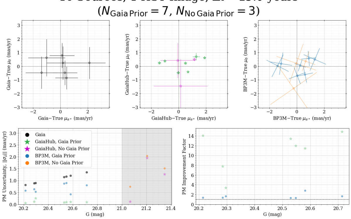
Finally, we explore the impact that the number of sources in an image have on the PM improvement factor when comparing BP3M to Gaia. An example analysis of a synthetic HST image with 10 sources and a 15 year time baseline is given in Figure 9. While the BP3M pipeline again finds good agreement with the truth, the median PM improvement factor over Gaia alone is only 1.39 for the sources in this synthetic image, which is much smaller than the median factor of 8.3 seen for the sources in the range of Figure 6. This is largely because the smaller number of sources aren’t able to place as strong a constraint on the transformation parameters’ distribution, and the larger transformation parameter distribution propagates to the PM distributions of individual sources.
Comparing the GaiaHub and BP3M panels, there is good agreement between the PM means for this particular realization of synthetic data, which should not be taken for granted considering the large GaiaHub outliers that can appear in real COSMOS data (e.g. of the PMs in Figure 2). When we compare the PM uncertainties, however, we see significant differences between the two pipelines. In fact, the GaiaHub uncertainties would need to be increased by a factor of 8 to explain the differences with the true PMs, while the BP3M PMs agree with the truth within their uncertainties. Some of the PM uncertainty differences come from the fact that the GaiaHub analysis is only able to propagate realistic transformation solution uncertainties to the final PMs if there are several HST images of the same field, which is not the case when considering a single synthetic image. The impact of the transformation uncertainty is likely negligible for relatively large numbers of sources (e.g. , as discussed in del Pino et al., 2022), but it becomes quite important in sparse fields and when there are only a handful of repeat HST observations of the same field (e.g. for many fields in COSMOS).
While it is fairly straightforward to estimate how much the GaiaHub uncertainties need to be inflated by using comparisons with the Gaia-measured PMs where they exist, it is much more difficult to assess and correct for the presence of systematics (e.g. as seen in the GaiaHub PMs of Figure 6) in sparse fields. Fortunately, these sparse halo conditions are what BP3M was developed for, and the synthetic data analysis provide evidence that the pipeline provides accurate PMs and uncertainties here.
We leave out example figures exploring the effect that a changing time baseline has on the posterior PMs because it follows expectations exactly; namely, for the same position uncertainty between two images, a smaller time baselines leads to larger PM uncertainties (e.g. Equation 2 of del Pino et al., 2022).
4.3 Optimizing Observing Strategies for Positions and Parallaxes
Our synthetic analysis also allows us to measure the improvement factors in the parallaxes and 2D position vectors of the sources. These results show, not unexpectedly, that the precision of these measurements is strongly tied (but not limited) to the magnitude of the source, the time baseline between images, the number of sources per image, and the effect of the position on the sky on the shape and orientation of the parallax motion. While we cannot change the time baselines of archival HST images, we can explore how changes in the observations times would have impacted the resulting BP3M parallaxes and positions. These lessons are particularly useful for planning of future observations using any telescope.

As before, we create synthetic HST images of COSMOS stars, but in this analysis, we do not let the HST position uncertainty of sources change as a function of magnitude based on GaiaHub examples (e.g. as discussed in Appendix B). Instead, we choose to set the HST position uncertainty to 0.01 pixels, which is the centroid uncertainty that previous studies have measured for well-behaved stars (e.g. Bellini et al., 2011). We adopt the single, well-behaved value to limit the effect that any particular choice/realization of position uncertainties may have on the conclusions we make about optimal observing strategies. Similarly, we choose to use 50 stars in each synthetic HST image to reduce the impact of transformation solution uncertainty as seen in low-source-count images.
Our initial tests suggest that there is minimal improvement on the Gaia-measured parallax or position vectors when using only one HST image (i.e. one HST in combination with Gaia). Additionally, multiple HST images taken very nearby in time (e.g. the multiple exposures taken to guard against cosmic rays) effectively act as a single epoch and are useful for improving the position uncertainty, but don’t offer much information to the parallax. When multiple HST images with common targets and substantial enough time baselines are analysed together, then the parallaxes and positions begin to show improvement. To better understand how parallax and position precision depend on observation times, we choose to simulate 3 epochs of COSMOS observations with HST, with time offsets from Gaia near 12, 8, and 4 years. Specifically, we make the observations occur at the following times:
-
1.
No Gaia Offset: All HST observations at year-multiples of the Gaia observation time,
; -
2.
Half Gaia Offset: All HST observations at half-a-year offset from the Gaia date, ;
-
3.
Apocenter-then-Quarter: The earliest HST observations at the parallax orbit apocenter farthest from Gaia, then offset by a quarter year for the other epochs,
; -
4.
Alternating Apocenters: The earliest HST observations at the parallax orbit apocenter farthest from Gaia, then alternating offsets by half a year for the other epochs,
.
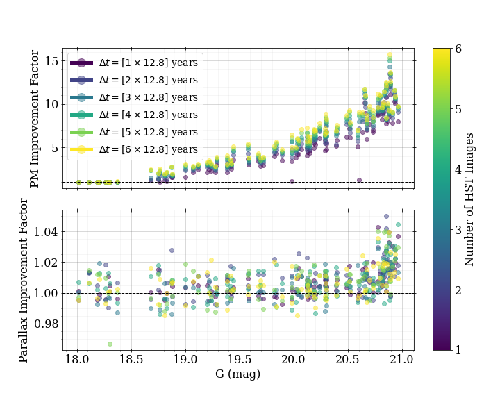
The resulting position, parallax, PM uncertainties from analysing these HST observations concurrently is given in Figure 10, where the two bottom-most panels show the 3D (i.e. parallax, PM) and 5D (i.e. position, parallax, PM) vector uncertainties. This figure reveals many important lessons about the impact that relatively small time offsets of observations within a year have on the stellar measurements.
From the top three panels, we see that different observing strategies lead to significant differences in the resulting position and parallax precisions, though there are minimal differences between the PM uncertainties. This implies that improvements in parallax and position can be achieved with no cost to the PM precision. We emphasize, however, that this is only after analysing all 3 HST epochs together; when considering a single epoch at a time, sources without Gaia priors (i.e. ) do indeed have significantly larger PM uncertainties if there is an offset from the Gaia date as a result of the degeneracy between PM and parallax motions. Our results suggest that completed surveys with multiple HST epochs may be able to improve position and parallax measurements for free through careful design.
Of the observing strategies we consider (including many that are not represented in Figure 10), the best choice for improving positions and parallaxes was to use an alternating-parallax-orbit-apocenters approach, which is the 4th option in the list above and the red points in the figure. This strategy suggests that the parallax is most improved – and therefore the degeneracy between PM and parallax motions most disentangled – when we consider the average parallax orbit of the sources in a given field (e.g. the blue orbit in Figure 3 for COSMOS). The parallax ellipse can be used to identify the points in time that are most distant from each other (i.e. the extremes of the semi-major axis), which are therefore the easiest to tell apart for a given position uncertainty. Then, the best approach is to first observe at the time that is most offset from the Gaia observation time, and subsequent observations alternate by half a year such that they jump back and forth between the two apocenters. This approach also appears to have a large improvement on the position uncertainty, likely caused by the repeated sampling of the source’s position at the same time in the parallax orbit.
5 Applications with Real Data
We test the pipeline using real data in four key ways: (1) using well-studied nearby dwarf spheroidal (dSph) galaxies, (2) using cross-matches with an external QSO catalog, (3) using cross-matches with a PM catalog in COSMOS derived from multi-epoch HST imaging, and (4) using the full unique COSMOS sources presented in Section 2.1.
5.1 Comparison with Nearby Dwarf Spheroidals


We analyse HST images using BP3M in nearby dSph galaxies to see how the posterior PMs and parallaxes compare to Gaia. This serves as a test with real data, as well as more proof that BP3M is improving the astrometric solutions for the sources it measures. We also show how analysing multiple HST images together impact the resulting PM and parallax precision.
A comparison of Gaia, GaiaHub, and BP3M measured PMs is presented in Figure 12 for the Fornax dwarf spheroidal. For the BP3M PMs, 6 HST images at the same epoch (time baseline from Gaia of 12.8 years) with a total of 198 unique sources are analysed together. The GaiaHub PMs are the same as in presented in del Pino et al. (2022) from analysis of the same 6 HST images, but in this case, a co-moving sample has been defined before transformation fitting to identify likely cluster members. While this figure is similar to Figure 6, the top panels are slightly different in that they show PM measurements instead of offsets from known PMs of synthetic data. Sources without Gaia-measured parallaxes and PMs are colored orange in the BP3M panel, which show larger uncertainties than the sources with Gaia priors in blue. The axes of the GaiaHub and BP3M panels have been set to cover the same range of values for easier visual comparison, and this range is times smaller than in the Gaia panel. As before, the lower panels compare the PM uncertainties. Figure 12 shows another PM comparison, this time using 10 HST images of the Draco dwarf spheroidal, taken at 3 different epochs (baselines of 11.2, 9.2, and 2.2 years from Gaia).
First, these figures show a significant tightening of the PMs when Gaia and HST are combined using either GaiaHub or BP3M. This suggests that the increase in PM precision over Gaia alone is not at the cost of PM accuracy. In comparing the PM uncertainties, we find that the GaiaHub values are slightly smaller than those of BP3M, but this is likely because BP3M propagates transformation parameter uncertainties to the final PMs and GaiaHub uses a single set of values for the transformation solution. We also see that the GaiaHub PMs form visually-tighter PM knots than the BP3M PMs, though we would expect them to be more similar based on the size of their PM uncertainties. These differences suggest that there are systematics in the BP3M PMs that are not present in the GaiaHub PMs. In testing possible explanations, we find that the BP3M results are able to look more like the GaiaHub ones when we restrict the samples to only the cluster members from del Pino et al. (2022). Theoretically, the BP3M statistics should not allow the presence of non-member sources to impact the PMs of member stars – in fact, their presence should help improve the transformation solution – but we find that this is not the case.
Some further testing suggests the likely culprit comes from BP3M’s estimate of the source position uncertainty in the HST images. As discussed previously, BP3M uses the same HST position uncertainties as GaiaHub, and this is calculated as a fraction of a PSF quality of fit statistic. When analysing a kinematically-cleaned, co-moving population of stars (i.e. the case that GaiaHub was designed for), this estimate of uncertainty performs well because the sample is restricted to faint sources that follow a linear relation between the quality of PSF fitting and HST position uncertainty. The validity of this approximation is evident from the resulting GaiaHub PMs and the results when BP3M uses the same subsample. However, this uncertainty approximation can occasionally underestimate the true uncertainty – especially for bright-but-not-saturated sources – leading to cases where the transformation solution becomes torqued away from the truth by a few unfairly-high-weighted sources. As more HST images are analysed together (e.g. as we present here with the dSph data), the amount that HST information contributes to the posterior measurements begins to outweigh the Gaia-measured priors, and it becomes more important for the HST uncertainties to be more accurate. It will be important for future versions of BP3M to identify other methods of measuring the HST position uncertainties to be as statistically robust as possible.
For all the BP3M analyses presented in this work, we emphasize that we use all Gaia sources found in each HST image to test the general nature of the pipeline. Our goal is to retain as many sources as possible for transformation fitting, which is especially important in sparse field cases. For BP3M, foreground bright stars – which often have well-measured Gaia positions, parallaxes, and PMs – that do not belong to the distant populations of interest are often useful anchors for the transformation fitting.
We next repeat the BP3M analysis while varying the number of HST images considered together to explore the effect this has on the posterior PMs and parallaxes. The resulting improvement factors as a function of magnitude are given in Figures 13 and 14 for Fornax and Draco respectively, with the legend displaying the time baselines from Gaia for the different sets of HST images. In the case of Fornax, the most significant improvement in PM occurs when analysing a single HST image with Gaia (i.e. a median PM precision increase by a factor of for ), though there is still an additional improvement when the remaining five HST images are brought in ( improvement for for ). The parallax uncertainties, however, do not improve very significantly for any of the images, though there is a slight, , precision increase at the faintest magnitudes. This is likely because the HST images are taken at a single epoch and the time baseline is quite close to a one year multiple of Gaia’s observation date (i.e. only offset by 20% of a year); this means that the parallax orbit is being sampled repeatedly in a small area at the same approximate time, which does not lead to significant increases in parallax precision.
For Draco, increasing the number of HST images does substantially improve the PMs for each image added; considering 10 HST images together with Gaia improves the PM precision by a median factor of for compared to a median factor of when only one HST image is used. The parallaxes also see a noticeable change in precision as a function of HST images analysed. While the time offsets from Gaia are again only of a year, the HST images are spread over three epochs. In the case of Fornax, we effectively have measurements of positions for each source at two different times (i.e. a single epoch of HST images plus Gaia) while the Draco data have measurements of positions at four different times; for the Draco stars then, there is smaller set of parallax and PM combinations that can explain those four position measurements per source than if there were only two position measurements. It is likely that the improvement in the parallax precision also contributes to the increase in PM precision because the degeneracy between the different types of apparent motion become less entangled. However, the time offsets of the HST images from Gaia and from each other are not optimally spaced in the parallax orbit (i.e. near the apocenters), resulting in a median parallax precision increase by a factor of for the faintest magnitudes ().
5.2 Comparison with QSOs


As an additional method of validating the BP3M posterior PMs and their uncertainties, we cross-match the unique COSMOS sources mentioned in Section 2 with the MILLIQUAS QSO catalog444https://heasarc.gsfc.nasa.gov/W3Browse/all/milliquas.html (Flesch, 2023). There are 52 sources in the QSO list that have COSMOS sources within , so we run the HST images that contain these sources through the BP3M pipeline, with the resulting posterior PMs shown in Figure 15. As expected for extremely distant sources, the PMs are closely distributed around the origin.
Next, we use the PM uncertainties to measure the 2D distances of the PMs from stationary, and then compare these measurements to the expected distribution; the result of this process is shown in Figure 16. The expected distribution (orange histogram) for an equivalent sample size agrees quite well with the measured one (blue histogram). This is additional and external evidence that the BP3M posterior PM distributions are reasonable and trustworthy.
5.3 Comparison with HST-measured PMs
Like in Section 5.2, we identify sources in our COSMOS sample that are shared with an external survey; in this case, we cross-match with the COSMOS sample of the HALO7D survey (Cunningham et al., 2019a, b; McKinnon et al., 2023). The HALO7D PMs are described in Cunningham et al. (2019b); to summarize, the PMs are measured using multiple epochs of HST imaging with the absolute reference frame being defined by registration with background galaxies. These HST+HST PMs are therefore a result of traditional PM measurement techniques.
We analyse the HST images in the multi-epoch region of COSMOS that have Gaia sources in common with the HALO7D survey, finding 31 cross-matches. In Figure 17, we see that the BP3M PMs have strong agreement with their HST-only counterparts. As in the other comparisons we have presented, the distribution of 2D differences between the PM measurements agree statistically with our expectations, providing the final piece of validation for the BP3M outputs.
5.4 Proper Motions in Sparse Fields: COSMOS


Using the HST images of the COSMOS field discussed in Section 2.1, we run BP3M on all images within of the field’s center. This includes all regions of COSMOS with multi-epoch HST imaging (near the center), as well as single-epoch-only HST regions. The posterior PMs we measure for the 2640 unique sources that are found in common between the HST images and Gaia are shown in Figure 18, where the sources are colored by whether or not they have Gaia-measured PMs and parallaxes. As a quick sanity check, this PM distribution visually agrees with our expectations based on the synthetic COSMOS data created using previously-measured velocity distributions for the MW thick disk and stellar halo555See Figure 23 in Appendix B, but note that our “visual comparison” here means looking at the range and spread of the PMs, not comparing the different colored populations in each figure.. There may be, however, more BP3M PMs clustered at the origin than originally expected (i.e. the orange, “No Gaia Prior” points), but many of these sources may truly be background stationary sources, which were not included as a component of the synthetic data.
While each source may appear in multiple HST frames, we only show the results from analysing each HST image separately, and the displayed PM is from the posterior distribution with the smallest uncertainty. Currently, it is very computationally expensive to analyse multiple HST concurrently, making the complete simultaneous analysis of COSMOS HST images intractable. Fortunately, as we determined from our dSph test data, analyses of single HST images do not show noticeable systematics in BP3M PMs as a result of the HST position uncertainty estimates, so the PMs we present for the COSMOS sample are robust. After increasing computation efficiency and HST position uncertainty estimates in planned updates to the pipeline, we will be able to present a complete COSMOS analysis in future work.
We also compare the BP3M PMs and uncertainties to the corresponding Gaia PMs in Figure 19, where we again see excellent agreement between the two samples (top panels). Because the sources in this figure include the same sources shown in Figure 2, we can also compare the sparse-field PM performance between the GaiaHub and BP3M pipelines. In general, BP3M returns much closer agreement with the Gaia PMs, as is expected because it uses those measurements as prior constraints. In addition, BP3M is able to measure consistent PMs for all 2640 Gaia sources in the COSMOS images, which is a large increase from the 1659 PMs catalog of GaiaHub. These results suggest that BP3M’s approach has successfully addressed the issues producing the outliers of Figure 19, indicating it is a valid method of extracting useful and trustworthy PMs in sparse fields.
The middle and bottom panels of Figure 19 show the improvement on the PM uncertainty that BP3M measures by combining HST and Gaia, especially for the of sources that had no Gaia-measured PMs; the median PM uncertainty for sources without Gaia priors is found to be . While many of the brightest magnitude sources – those most likely to be at or near saturation in the HST images – show no improvement on Gaia’s PMs, the faintest magnitude sources () have a median PM improvement factor of 2.6. As mentioned for the small-source-count case in Figure 9, the less extreme improvements in PM we see in sparse fields are likely the result of larger uncertainty in the transformation parameters, which propagates to the PM uncertainties of all sources in an image.
The BP3M transformation parameters could likely be pinned down much more precisely by identifying stationary sources in each image. For example, by finding the centroids in each HST image that are clearly associated with quasars and background galaxies, then updating the priors in parallax and PM to a narrow distribution around , the transformation solution can be improved by these anchor points. This would reduce the posterior width of the transformation parameter distributions for each image, especially for particularly sparse images, which would also reduce the posterior widths in the PMs for all of the sources in an HST image. Exploring the impact that known stationary targets can have on the BP3M PMs will be the focus of future work.
The median PM uncertainties in the range are summarized for the COSMOS sample in Table 2. First, the BP3M sample that has Gaia parallax and PM priors has a significant increase in precision compared to Gaia alone. Second, the Gaia COSMOS sample () has a similar median PM uncertainty to the BP3M sample without Gaia priors (), but the latter contains significantly more stars. Effectively, BP3M substantially increases the number of stars in a single field with Gaia-quality PMs at the faintest magnitudes.
| Number of | Median | |
| Sample | Sources | (mas/yr) |
| Gaia | 443 | 1.03 |
| BP3M, Gaia Prior | 443 | 0.44 |
| BP3M, No Gaia Prior | 632 | 1.13 |
A typical MW stellar halo isochrone (i.e. and , see Appendix B) has a red giant branch (RGB) base around an absolute magnitude of . For stars at the base of the RGB with apparent magnitudes in the range, this translates to a distance range of . Using the median PM uncertainties in Table 2, this would imply an uncertainty in velocity on the sky in the range of for the Gaia-alone sample versus a range for the BP3M sample with Gaia priors. For the BP3M sample without Gaia priors, the apparent magnitude range of translates to a distance range of , and results in a sky velocity uncertainty range of when using the median PM uncertainty for this subsample.
Like with the dwarf spheroidal data, many of these COSMOS sources appear in multiple HST images. As a result, the BP3M PM uncertainties presented in this section are significantly larger than the possible PM uncertainty that could be achieved by analysing the images concurrently, which will be the focus on future work. This may also likely yield improvements on the parallax precision, especially for sources in the multi-epoch HST regions of the field. Finally, there are many HST sources that are too faint to have Gaia counterparts, but they nonetheless appear in multiple HST frames. For these sources, future versions of BP3M can use the HST-to-Gaia transformation parameters for each image to identify the positions of these sources in a global reference frame as a function of time, and thus determine their best fit PMs and parallaxes.
In tests of a handful of COSMOS images where we analyse all overlapping HST concurrently, we measure a median PM uncertainty of for mag (sources with Gaia-measured PMs) and a median PM uncertainty of for mag (sources with Gaia-measured PMs). In future work, we plan to use the extreme precision PMs to investigate substructure in the MW stellar halo at large distances ( kpc). Other future applications including measuring internal kinematics of perturbed stellar streams – whose stars are often in sparse fields that are analogous to COSMOS, and where the 3D velocity error budget is dominated by PM terms (e.g., GD-1 Price-Whelan & Bonaca, 2018; Malhan & Ibata, 2019) – to constrain the dark matter subhalo mass function.
6 Summary
We have presented the statistics that describe, in general, how positions of sources from two or more sets of images (from any telescope or instrument) should be combined in a Bayesian hierarchical framework to measure transformation parameters between the images, as well as distributions on the positions, parallaxes, and PMs for the individual sources. We use these statistics to created BP3M – a pipeline that builds off of GaiaHub – to combine archival HST and Gaia data to measure reliable positions, parallaxes, and PMs in the absolute reference frame of Gaia, even in sparse fields (e.g. per HST image). We have tested this pipeline using a combination of synthetic HST images, nearby dwarf galaxies, a catalog of QSOs, and sparse MW stellar halo fields. In all cases, we find that the BP3M PMs are both accurate and precise, especially for magnitudes where Gaia has large PM uncertainties () or no PM measurements at all ().
Our key results include:
-
1.
When trying to maximize parallax precision, the best observing strategy we have found is to alternate the observation times between the two semi-major axis extremes of the ellipse created by the parallax motion. The improvement to the parallax and position precision come at no cost to the PM uncertainty (Section 4.3, Figures 10);
- 2.
- 3.
References
- Anderson (2007) Anderson, J. 2007, Variation of the Distortion Solution, Instrument Science Report ACS 2007-08, 12 pages
- Anderson (2022) —. 2022, One-Pass HST Photometry with hst1pass, Instrument Science Report WFC3 2022-5, 55 pages
- Anderson & King (2004) Anderson, J., & King, I. R. 2004, Multi-filter PSFs and Distortion Corrections for the HRC, Instrument Science Report ACS 2004-15, 51 pages
- Anderson & King (2006) —. 2006, PSFs, Photometry, and Astronomy for the ACS/WFC, Instrument Science Report ACS 2006-01, 34 pages
- Astropy Collaboration et al. (2013) Astropy Collaboration, Robitaille, T. P., Tollerud, E. J., et al. 2013, A&A, 558, A33, doi: 10.1051/0004-6361/201322068
- Astropy Collaboration et al. (2018) Astropy Collaboration, Price-Whelan, A. M., Sipőcz, B. M., et al. 2018, AJ, 156, 123, doi: 10.3847/1538-3881/aabc4f
- Astropy Collaboration et al. (2022) Astropy Collaboration, Price-Whelan, A. M., Lim, P. L., et al. 2022, apj, 935, 167, doi: 10.3847/1538-4357/ac7c74
- Bellini et al. (2011) Bellini, A., Anderson, J., & Bedin, L. R. 2011, PASP, 123, 622, doi: 10.1086/659878
- Bellini et al. (2017) Bellini, A., Anderson, J., Bedin, L. R., et al. 2017, ApJ, 842, 6, doi: 10.3847/1538-4357/aa7059
- Bellini & Bedin (2009) Bellini, A., & Bedin, L. R. 2009, PASP, 121, 1419, doi: 10.1086/649061
- Bellini et al. (2018) Bellini, A., Libralato, M., Bedin, L. R., et al. 2018, ApJ, 853, 86, doi: 10.3847/1538-4357/aaa3ec
- Belokurov et al. (2018) Belokurov, V., Erkal, D., Evans, N. W., Koposov, S. E., & Deason, A. J. 2018, MNRAS, 478, 611, doi: 10.1093/mnras/sty982
- Bennet et al. (2022) Bennet, P., Alfaro-Cuello, M., Pino, A. d., et al. 2022, ApJ, 935, 149, doi: 10.3847/1538-4357/ac81c9
- Bonaca et al. (2020) Bonaca, A., Conroy, C., Cargile, P. A., et al. 2020, ApJ, 897, L18, doi: 10.3847/2041-8213/ab9caa
- Choi et al. (2016) Choi, J., Dotter, A., Conroy, C., et al. 2016, ApJ, 823, 102, doi: 10.3847/0004-637X/823/2/102
- Conroy et al. (2019) Conroy, C., Naidu, R. P., Zaritsky, D., et al. 2019, ApJ, 887, 237, doi: 10.3847/1538-4357/ab5710
- Cunningham et al. (2019a) Cunningham, E. C., Deason, A. J., Rockosi, C. M., et al. 2019a, ApJ, 876, 124, doi: 10.3847/1538-4357/ab16cb
- Cunningham et al. (2023) Cunningham, E. C., Hunt, J. A. S., Price-Whelan, A. M., et al. 2023, arXiv e-prints, arXiv:2307.08730, doi: 10.48550/arXiv.2307.08730
- Cunningham et al. (2019b) Cunningham, E. C., Deason, A. J., Sanderson, R. E., et al. 2019b, ApJ, 879, 120, doi: 10.3847/1538-4357/ab24cd
- Cunningham et al. (2022) Cunningham, E. C., Sanderson, R. E., Johnston, K. V., et al. 2022, ApJ, 934, 172, doi: 10.3847/1538-4357/ac78ea
- del Pino et al. (2022) del Pino, A., Libralato, M., van der Marel, R. P., et al. 2022, ApJ, 933, 76, doi: 10.3847/1538-4357/ac70cf
- Dotter (2016) Dotter, A. 2016, ApJS, 222, 8, doi: 10.3847/0067-0049/222/1/8
- Flesch (2023) Flesch, E. W. 2023, arXiv e-prints, arXiv:2308.01505, doi: 10.48550/arXiv.2308.01505
- Foreman-Mackey (2016) Foreman-Mackey, D. 2016, The Journal of Open Source Software, 1, 24, doi: 10.21105/joss.00024
- Foreman-Mackey et al. (2013) Foreman-Mackey, D., Hogg, D. W., Lang, D., & Goodman, J. 2013, PASP, 125, 306, doi: 10.1086/670067
- Gaia Collaboration et al. (2018) Gaia Collaboration, Helmi, A., van Leeuwen, F., et al. 2018, A&A, 616, A12, doi: 10.1051/0004-6361/201832698
- Grogin et al. (2011) Grogin, N. A., Kocevski, D. D., Faber, S. M., et al. 2011, ApJS, 197, 35, doi: 10.1088/0067-0049/197/2/35
- Harris et al. (2020) Harris, C. R., Millman, K. J., van der Walt, S. J., et al. 2020, Nature, 585, 357, doi: 10.1038/s41586-020-2649-2
- Helmi et al. (2018) Helmi, A., Babusiaux, C., Koppelman, H. H., et al. 2018, Nature, 563, 85, doi: 10.1038/s41586-018-0625-x
- Hunter (2007) Hunter, J. D. 2007, Computing in Science & Engineering, 9, 90, doi: 10.1109/MCSE.2007.55
- Iorio & Belokurov (2021) Iorio, G., & Belokurov, V. 2021, MNRAS, 502, 5686, doi: 10.1093/mnras/stab005
- Kluyver et al. (2016) Kluyver, T., Ragan-Kelley, B., Pérez, F., et al. 2016, in Positioning and Power in Academic Publishing: Players, Agents and Agendas, ed. F. Loizides & B. Schmidt, IOS Press, 87 – 90
- Koekemoer et al. (2011) Koekemoer, A. M., Faber, S. M., Ferguson, H. C., et al. 2011, ApJS, 197, 36, doi: 10.1088/0067-0049/197/2/36
- Kroupa (2001) Kroupa, P. 2001, MNRAS, 322, 231, doi: 10.1046/j.1365-8711.2001.04022.x
- Libralato et al. (2019) Libralato, M., Bellini, A., Piotto, G., et al. 2019, ApJ, 873, 109, doi: 10.3847/1538-4357/ab0551
- Libralato et al. (2018) Libralato, M., Bellini, A., van der Marel, R. P., et al. 2018, ApJ, 861, 99, doi: 10.3847/1538-4357/aac6c0
- Libralato et al. (2022) Libralato, M., Bellini, A., Vesperini, E., et al. 2022, ApJ, 934, 150, doi: 10.3847/1538-4357/ac7727
- Lindegren et al. (2018) Lindegren, L., Hernández, J., Bombrun, A., et al. 2018, A&A, 616, A2, doi: 10.1051/0004-6361/201832727
- Luri et al. (2018) Luri, X., Brown, A. G. A., Sarro, L. M., et al. 2018, A&A, 616, A9, doi: 10.1051/0004-6361/201832964
- Mackereth et al. (2019) Mackereth, J. T., Schiavon, R. P., Pfeffer, J., et al. 2019, MNRAS, 482, 3426, doi: 10.1093/mnras/sty2955
- Malhan & Ibata (2019) Malhan, K., & Ibata, R. A. 2019, MNRAS, 486, 2995, doi: 10.1093/mnras/stz1035
- Massari et al. (2018) Massari, D., Breddels, M. A., Helmi, A., et al. 2018, Nature Astronomy, 2, 156, doi: 10.1038/s41550-017-0322-y
- Massari et al. (2020) Massari, D., Helmi, A., Mucciarelli, A., et al. 2020, A&A, 633, A36, doi: 10.1051/0004-6361/201935613
- Massari et al. (2017) Massari, D., Posti, L., Helmi, A., Fiorentino, G., & Tolstoy, E. 2017, A&A, 598, L9, doi: 10.1051/0004-6361/201630174
- McKinnon et al. (2023) McKinnon, K. A., Cunningham, E. C., Rockosi, C. M., et al. 2023, arXiv e-prints, arXiv:2302.07293, doi: 10.48550/arXiv.2302.07293
- Muzzin et al. (2013) Muzzin, A., Marchesini, D., Stefanon, M., et al. 2013, ApJS, 206, 8, doi: 10.1088/0067-0049/206/1/8
- Naidu et al. (2020) Naidu, R. P., Conroy, C., Bonaca, A., et al. 2020, ApJ, 901, 48, doi: 10.3847/1538-4357/abaef4
- Nayyeri et al. (2017) Nayyeri, H., Hemmati, S., Mobasher, B., et al. 2017, ApJS, 228, 7, doi: 10.3847/1538-4365/228/1/7
- pandas development team (2020) pandas development team, T. 2020, pandas-dev/pandas: Pandas, latest, Zenodo, doi: 10.5281/zenodo.3509134
- Paxton et al. (2011) Paxton, B., Bildsten, L., Dotter, A., et al. 2011, ApJS, 192, 3, doi: 10.1088/0067-0049/192/1/3
- Paxton et al. (2013) Paxton, B., Cantiello, M., Arras, P., et al. 2013, ApJS, 208, 4, doi: 10.1088/0067-0049/208/1/4
- Paxton et al. (2015) Paxton, B., Marchant, P., Schwab, J., et al. 2015, ApJS, 220, 15, doi: 10.1088/0067-0049/220/1/15
- Pérez & Granger (2007) Pérez, F., & Granger, B. E. 2007, Computing in Science and Engineering, 9, 21, doi: 10.1109/MCSE.2007.53
- Price-Whelan & Bonaca (2018) Price-Whelan, A. M., & Bonaca, A. 2018, ApJ, 863, L20, doi: 10.3847/2041-8213/aad7b5
- Robin et al. (2003) Robin, A. C., Reylé, C., Derrière, S., & Picaud, S. 2003, A&A, 409, 523, doi: 10.1051/0004-6361:20031117
- Schönrich et al. (2011) Schönrich, R., Asplund, M., & Casagrande, L. 2011, MNRAS, 415, 3807, doi: 10.1111/j.1365-2966.2011.19003.x
- Sohn et al. (2012) Sohn, S. T., Anderson, J., & van der Marel, R. P. 2012, ApJ, 753, 7, doi: 10.1088/0004-637X/753/1/7
- Sohn et al. (2018) Sohn, S. T., Watkins, L. L., Fardal, M. A., et al. 2018, ApJ, 862, 52, doi: 10.3847/1538-4357/aacd0b
- van de Ven et al. (2006) van de Ven, G., van den Bosch, R. C. E., Verolme, E. K., & de Zeeuw, P. T. 2006, A&A, 445, 513, doi: 10.1051/0004-6361:20053061
- van der Marel et al. (2012) van der Marel, R. P., Fardal, M., Besla, G., et al. 2012, ApJ, 753, 8, doi: 10.1088/0004-637X/753/1/8
- Vasiliev & Baumgardt (2021) Vasiliev, E., & Baumgardt, H. 2021, MNRAS, 505, 5978, doi: 10.1093/mnras/stab1475
- Virtanen et al. (2020) Virtanen, P., Gommers, R., Oliphant, T. E., et al. 2020, Nature Methods, 17, 261, doi: 10.1038/s41592-019-0686-2
- Wes McKinney (2010) Wes McKinney. 2010, in Proceedings of the 9th Python in Science Conference, ed. Stéfan van der Walt & Jarrod Millman, 56 – 61, doi: 10.25080/Majora-92bf1922-00a
Appendix A Motion Statistics
Here, we present the posterior conditional distributions in PM, parallax, and position for a given source.
Because of it’s lack of coefficients, it is easiest to solve for the posterior conditional on first:
| (A1) |
where we use bold-faced versions of scalars to represent the corresponding identity matrix version of that number, such as
We have also included a term for the Gaia-measured position offset vector to be as general as possible, but this vector is just because Gaia has no measured offset from the positions it reports.
Next, the posterior conditional on is given by:
| (A2) |
where
| (A3) |
| (A4) |
| (A5) |
| (A6) |
Finally, the posterior conditional on is given by:
| (A7) |
where
| (A8) |
| (A9) |
| (A10) |
| (A11) |
| (A12) |
| (A13) |
Because these three posterior conditional distributions are all Gaussian, we are able to quickly sample PMs, parallaxes, and position offsets for source given a set of transformation parameters.
| Component | Distribution | Functional Form |
|---|---|---|
| Halo | ||
| Kroupa (2001) IMF, with | ||
| with | ||
| Thick Disk | ||
| Kroupa (2001) IMF | ||
| , where | ||
Appendix B Generating Synthetic, COSMOS-like Data


Following a similar approach to McKinnon et al. (2023), we define mass, age, , and distance distributions for both a MW thick disk and a MW halo population. We also define distributions for the Galactocentric 3D velocities for the halo and thick disk. The distributions for each parameter that go into generating a synthetic star are summarized in Table 3. The particular choices for the velocity distributions come from the MW halo velocity ellipsoid measurements of Cunningham et al. (2019b), as do the distance modulus distributions. For the age distributions, we use an analytical approximation of the age distributions presented in Bonaca et al. (2020). The distributions are again analytical approximations of the results presented in Conroy et al. (2019) and Naidu et al. (2020). The age and distributions are displayed in Figure 20, where the distributions have been scaled by their contribution to the total halo population. After consulting a Besançon model (Robin et al., 2003) in a COSMOS-like field in the range, we choose to set the fraction of the number of observed stars that belong to the halo (i.e. “halo fraction”) to 28%.
Using these distributions and the halo fraction, we draw stellar parameters (i.e. mass, age, and ) for each synthetic star, and then interpolate to that point using the MIST isochrones777https://waps.cfa.harvard.edu/MIST/index.html (Dotter, 2016; Choi et al., 2016; Paxton et al., 2011, 2013, 2015). This interpolated point yields the color and absolute magnitude of each synthetic star. After we draw distances, we can measure the apparent magnitudes for each star, and then perform rejection sampling to get a sample of stars that fall within a particular range in magnitude and/or color. A color-magnitude diagram is shown in Figure 21 for the COSMOS-like stars we generate, with histograms along the top and right edges showing the distribution of the halo (purple), thick disk (turquoise), and total (lime green) populations. A histogram of the heliocentric distance to each synthetic star is given in Figure 22.
Next, for each synthetic star, we draw the 3D velocity components based on whether that star belongs to the halo or the thick disk. Using the stellar position on the sky and distance allow us to transform those Galactocentric velocities into observable velocities888To transform between the observer frame and a Galactocentric one, we use kpc, assume a circular speed of , and solar peculiar motion (Schönrich et al., 2011).. This yields the PMs shown in Figure 23.
To create outputs that the BP3M pipeline expects, the next step is to create synthetic HST images and corresponding Gaia measurements. For synthetic Gaia uncertainties on position, parallax, and PM, we look at real Gaia-measured stars within 1 degree of the COSMOS field center; the resulting uncertainties in each dimension are shown in Figure 24 as a function of magnitude (black points) with a median-binned line overlaid (red). In cases where the data do not extend as faint as needed, we linearly extrapolate from the median binning.
We use a similar approach when it comes to modeling the uncertainties in the HST image positions. Specifically, we use the real COSMOS stars from Section 5.4 to look at the GaiaHub-measured HST position uncertainties as a function of magnitude, and this is shown in Figure 25. When we go to assign HST position uncertainties to the synthetic stars, we identify the 10 nearest real COSMOS stars in magnitude and randomly select one of those stars to bequeath its position uncertainty to the synthetic one.
With all of the true properties of the synthetic star defined, we can create Gaia-like measurements of the position, parallax, and uncertainty by applying some noise corresponding to the uncertainties we’ve defined. Those true positions and motions can then be played forward or backward in time until reaching the correct epoch of the synthetic HST image. After choosing the transformation parameters that map the synthetic HST image onto the synthetic Gaia data, we can apply the correct HST position noise, and then save the outputs in the same .csv files that BP3M expects as inputs. The final step of the process is to run BP3M on the newly-generated synthetic HST images.