Boundary stabilization of a vibrating string with variable length

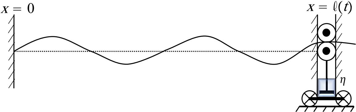
We consider small transversal vibrations of a uniform string, with a time dependent length. The mechanical setting is sketched in Figure 1 where the left end of the string is fixed while the right moving end is also allowed to move transversely and attached to a damping device (a dash-pot with a damping factor $\eta\geq 0$).

Denoting the displacement function by $u$, depending on the position $x$ along the string and the time $t$, the model can be stated as follows

The subscripts $t$ and $x$ in (WP) stand for the derivatives in time and space variables respectively. The functions $u^{0}$ and $u^{1}$ represents the initial shape and the initial transverse speed of the string, respectively. The initial length of the string is denoted by $L=\ell(0)$.

We assume that $\ell\in C\left(\left[0,+\infty\right[\right)$ and that

which means that the speed of variation of the length of the string $\ell^{\prime}\left(t\right)$ is strictly less then the speed of propagation of the wave (here simplified to $c=1$).

In this paper, we are mainly interested in the asymptotic behaviour in time of the energy of the solution, defined as

For the time-independent interval, i.e. when $\ell\left(t\right)=L$ for $t\geq 0$, it is well known that:

• •

  If $\eta=0$, then it is the energy is constant, i.e. $E_{L}\left(t\right)=E_{L}\left(0\right),$ for $t\geq 0$.

• •

  If $\eta\geq 0$ with $\eta\neq 1\$, then the energy decays exponentially

  $$E_{L}\left(t\right)\leq CE_{L}\left(0\right)e^{-\frac{1}{L}\ln\left|\gamma_{\eta}\right|t},\text{ for some constant }C>0,$$

  where $\gamma_{\eta}:=\frac{1+\eta}{1-\eta}$, see [15, 4, 3, 11]. In [5], the present authors showed that

  $$\frac{1}{\gamma_{\eta}^{2}}E_{L}\left(0\right)e^{-\frac{1}{L}\ln\left|\gamma_{\eta}\right|t}\leq E_{L}\left(t\right)\leq\gamma_{\eta}^{2}E_{L}\left(0\right)e^{-\frac{1}{L}\ln\left|\gamma_{\eta}\right|t},\ \ \ \text{for }t\geq 0.$$

  (1.3)

The question of $E_{\ell}\left(t\right)$ behaviour in time is more delicate if the interval depends on time. For instance, for the Dirichlet boundary conditions (which corresponds to $\eta=+\infty$ in (WP)), the energy decays if the interval is expanding and increases if the interval is shrinking, see [2]. See also [12, 13, 14] when the variation of the length is uniform in time.

Regarding the case with a velocity feedback at the moving endpoint $x=\ell\left(t\right)$:

• •

  Gugat [6] considered the case $u_{x}\left(\ell\left(t\right),t\right)+cu_{t}\left(\ell\left(t\right),t\right)=0$ where $c$ is as constant. See also [8] for the particular $\ell(t)=1+vt$ where $v$ is a constant, $0<v<1$.

• •

  Ammari et al. [1] considered the case $u_{x}\left(\ell\left(t\right),t\right)+f\left(t\right)u_{t}\left(\ell\left(t\right),t\right)=0,$ where $f\in L^{\infty}\left(0,+\infty\right)\$and $\ell\left(t\right)$ is periodic. See also [7] where $\ell\left(t\right)$ is not necessarily periodic. Mokhtari [9] considered the case with two moving endpoints.

For the special case $\eta=1$, the boundary condition at $x=\ell\left(t\right)$ reads

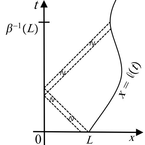
This is a transparent condition, i.e. there is no reflections of waves from the moving endpoint and consequently all the initial disturbances leave the interval $\left(0,\ell\left(t\right)\right)$ at most after a time

where $\beta\left(t\right):=t-\ell\left(t\right),$ see Figure 2. Hence, wether the interval is expanding or shrinking, the linear velocity feedback $-u_{t}\left(\ell^{\prime}\left(t\right),t\right)$ steers the solution to the zero state in the finite time $T_{\ell}$. See for instance [6, 7], and for the particular case $\ell\left(t\right)=L$ see [15, 4]. In the remaining of this paper, we will assume that $\eta\geq 0$ and $\eta\neq 1.$

The approach used in the paper at hands is based on generalized Fourier series. This is possible since the closed form for the solution of (WP) is given by the series

where the coefficients $c_{n}$ can be explicitly computed in function of the initial data $u^{0},u^{1}.\$We denoted by $\omega_{n}$ a sequence of complex number given by

Observe that since $\left|\gamma_{\eta}\right|\geq 1$ for every $\eta\geq 0,$ the real part of $\omega_{n}$ is nonpositive.

By $\varphi,$ we denoted a real function satisfying the functional equation

This equation often called Moor’s equation following his paper [10]. Some pairs of solutions $(\ell,\phi)$ can be found in [17].

We will assume that $\varphi$ is differentiable and increasing. More precisely,

The assumption $\varphi^{\prime}>0$ is needed in the sequel since $\varphi^{\prime}$ will serve as a weight for an $L^{2}$ space. Besides, a deacreasing $\phi$ can not satisfy (1.6) since $\ell\left(t\right)>0$. See [7] for further discussions on the regularity of the solutions of (1.6).

In this work, we demonstrate how the series formulas (1.4) can be used to achieve the following results:

• •

  For the undamped case, i.e. $\eta=0$, the energy of the solution satisfies

  $$\frac{m\left(t\right)}{M\left(t_{0}\right)}E_{\ell}\left(t_{0}\right)\leq E_{\ell}\left(t\right)\leq\frac{M\left(t\right)}{m\left(t_{0}\right)}E_{\ell}\left(t_{0}\right),\text{ \ \ \ for }0\leq t_{0}<t,$$

  (1.8)

  where

  $$m\left(t\right):=\min_{x\in\left[0,\ell\left(t\right)\right]}\left\{\varphi^{\prime}(t-x),\varphi^{\prime}(t+x)\right\}\ \text{and }M\left(t\right):=\max_{x\in\left[0,\ell\left(t\right)\right]}\left\{\varphi^{\prime}(t-x),\varphi^{\prime}(t+x)\right\}.$$

  (1.9)

  See Theorem 2 and its corollaries for sharper estimates.

• •

  For the damped case $\eta>0,$ with $\eta\neq 1$, the energy $E_{\ell}\left(t\right)$ satisfies

  $$\left(\frac{e^{\ln\left|\gamma_{\eta}\right|\varphi(t_{0}-\ell\left(t_{0}\right))}}{M\left(t_{0}\right)}\right)m\left(t\right)e^{-\ln\left|\gamma_{\eta}\right|\varphi(t+\ell\left(t\right))}E_{\ell}\left(t_{0}\right)\leq E_{\ell}\left(t\right)\\ \leq\left(\frac{e^{\ln\left|\gamma_{\eta}\right|\varphi(t_{0}+\ell\left(t_{0}\right))}}{m\left(t_{0}\right)}\right)M\left(t\right)e^{-\ln\left|\gamma_{\eta}\right|\varphi(t-\ell\left(t\right))}E_{\ell}\left(t_{0}\right),\text{ \ for }0\leq t_{0}<t.$$

  (1.10)

  See Theorem 3 and it corollaries for more estimates. The estimate given in (1.10), with explicit constants, is new to the best to our knowledge.

After the present introduction, we derive the exact solution and the expression for the coefficients of the series formula (1.4). In Section 3, we establish upper and lower estimates for the energy $E_{\ell}(t)$ of the undamped equation. In Section 4, we deal with the damped case. Some examples will be included as a last section.

Let us introduce the following family of Hilbert spaces

and assume that the initial data satisfies

Let $T>0.$ Then, we have the following existence result for Problem (WP).

In this section, we show some results for the undamped case, i.e. $\eta=0$ in Problem (WP). To know wether the energy is increasing or in creasing, we compute $E_{\ell}^{\prime}\left(t\right).$ Thus, using Leibniz’s rule for differentiation under the integral sign, we get

Since $u_{tt}=u_{xx}$ , then $u_{t}u_{tt}+u_{x}u_{tx}=\left(u_{t}u_{x}\right)_{x}\$and it follows

Then, we have the following result.

The next theorem show that the asymptotic behaviour of $E_{\ell}\left(t\right)$ is dictated by $\varphi^{\prime}.$

References

- [1] K. Ammari, A. Bchatnia, and K. El Mufti. Stabilization of the wave equation with moving boundary. Eur. J. Control, 39:35–38, 2018. ISSN 0947-3580.
- [2] C. Bardos and G. Chen. Control and stabilization for the wave equation. III: Domain with moving boundary. SIAM J. Control Optim., 19:123–138, 1981.
- [3] M. Cherkaoui. Estimation optimale du taux de décroissance de l’énergie pour une équation des ondes avec contrôle frontière. Rapport de recherche N°2328 - INRIA, 1994.
- [4] S. Cox and E. Zuazua. The rate at which energy decays in a string damped at one end. Indiana Univ. Math. J., pages 545–573, 1995.
- [5] S. E. Ghenimi and A. Sengouga. Energy decay estimates for an axially travelling string damped at one end. Submitted. URL http://arxiv.org/abs/2211.10537. 14 pages.
- [6] M. Gugat. Optimal boundary feedback stabilization of a string with moving boundary. IMA J. Math. Control Inform., 25(1):111–121, 2008.
- [7] B. H. Haak and D.-T. Hoang. Exact observability of a 1-dimensional wave equation on a noncylindrical domain. SIAM J. Control Optim., 57(1):570–589, 2019.
- [8] L. Lu and Y. Feng. Observability and stabilization of wave equations with moving boundary feedback. Acta Appl. Math., 170(1):731–753, 2020.
- [9] Y. Mokhtari. Boundary controllability and boundary time-varying feedback stabilization of the 1d wave equation in non-cylindrical domains. Evol. Equ. Control Theory, 11(2):373–397, 2022.
- [10] G. T. Moore. Quantum theory of electromagnetic field in a variable-length one-dimensional cavity. J. Math. Phys., 11(9):2679–2691, 1970.
- [11] J. P. Quinn and D. L. Russell. Asymptotic stability and energy decay rates for solutions of hyperbolic equations with boundary damping. Proc. R. Soc. Edinb. A: Math., 77(1-2):97–127, 1977.
- [12] A. Sengouga. Observability of the 1-D wave equation with mixed boundary conditions in a non-cylindrical domain. Mediterr. J. Math., 15(62):1–22, 2018.
- [13] A. Sengouga. Observability and controllability of the 1-D wave cquation in domains with moving boundary. Acta Appli. Math., 157:117–128, 2018.
- [14] H. Sun, H. Li, and L. Lu. Exact controllability for a string equation in domains with moving boundary in one dimension. Electron. J. Diff. Equations, 2015(98):1–7, 2015.
- [15] K. Veselić. On linear vibrational systems with one dimensional damping. Appl. Anal., 29(1-2):1–18, 1988.
- [16] A. I. Vesnitskii. The inverse problem for a one-dimensional resonator the dimensions of which vary with time. Radiophysics and Quantum Electronics, 14(10):1209–1215, 1971.
- [17] A. I. Vesnitskii and A. I. Potapov. Some general properties of wave processes in one-dimensional mechanical systems of variable length. Sov. App. Mechanics, 11(4):422–426, 1975. ISSN 1573-8582.