Boundary controllability of the Korteweg-de Vries equation: The Neumann case

Roberto de A. Capistrano Filho Departamento de Matemática, Universidade Federal de Pernambuco (UFPE), 50740-545, Recife (PE), Brazil, www.ufpe.br/capistranofilho ([email protected]). Jandeilson Santos da Silva ) Departamento de Matemática, Universidade Federal de Pernambuco (UFPE), 50740-545, Recife (PE), Brazil ([email protected]

Abstract

This article gives a necessary first step to understanding the critical set phenomenon for the Korteweg-de Vries (KdV) equation posed on interval $[0,L]$ considering the Neumann boundary conditions with only one control input. We showed that the KdV equation is controllable in the critical case, i.e., when the spatial domain $L$ belongs to the set $\mathcal{R}_{c}$ , where $c\neq-1$ and

\mathcal{R}_{c}:=\left\{\frac{2\pi}{\sqrt{3(c+1)}}\sqrt{m^{2}+ml+m^{2}};\ m,l\in\mathbb{N}^{*}\right\}\cup\left\{\frac{m\pi}{\sqrt{c+1}};\ m\in\mathbb{N}^{*}\right\},

the KdV equation is exactly controllable in $L^{2}(0,L)$ . The result is achieved using the return method together with a fixed point argument.

keywords:

Korteweg–de Vries equation, exact boundary controllability, Neumann boundary conditions, Dirichlet boundary conditions, critical set

{AMS}

Primary, 35Q53, 93B05; Secondary, 37K10

1 Introduction

We had known when we formulated the waves as a free boundary problem of the incompressible, irrotational Euler equation in an appropriate non-dimensional form, there exist two non-dimensional parameters $\delta:=\frac{h}{\lambda}$ and $\varepsilon:=\frac{a}{h}$ , where the water depth, the wavelength and the amplitude of the free surface are parameterized as $h,\lambda$ and $a$ , respectively. See, for instance, [2, 3, 1, 4, 23, 26] and references therein for a rigorous justification. Moreover, another non-dimensional parameter $\mu$ appears, the Bond number, to measure the importance of gravitational forces compared to surface tension forces also appears. Considering the physical condition $\delta\ll 1$ we can characterize the waves, called long waves or shallow water waves. In particular, considering the relations between $\varepsilon$ and $\delta$ , we can have the following regime:

•

Korteweg-de Vries (KdV): $\varepsilon=\delta^{2}\ll 1$ and $\mu\neq\frac{1}{3}$ . Under this regime, Korteweg and de Vries [20]¹¹1This equation was first introduced by Boussinesq [6], and Korteweg and de Vries rediscovered it twenty years later. derived the following well-known equation as a central equation among other dispersive or shallow water wave models called the KdV equation from the equations for capillary-gravity waves:

$\pm 2\eta_{t}+3\eta\eta_{x}+\left(\frac{1}{3}-\mu\right)\eta_{xxx}=0.$

Today, it is well known that this equation has an important phenomenon that directly affects the control problem related to them, the so-called critical length phenomenon. Let us briefly present the control problem, which makes the phenomenon of critical lengths emerge. The control problem was presented in a pioneering work of Rosier [24] that studied the following system

\left\{\begin{array}[c]{lll}u_{t}+u_{x}+uu_{x}+u_{xxx}=0,&&\text{ in }(0,L)\times(0,T),\\ u(0,t)=0,\text{ }u(L,t)=0,\text{ }u_{x}(L,t)=g(t),&&\text{ in }(0,T),\\ u(x,0)=u_{0}(x),&&\text{ in }(0,L),\end{array}\right.

(1.1)

where the boundary value function $g(t)$ is considered as a control input. Precisely, the author showed the following control problem for the system (1.1), giving the origin of the critical length phenomenon for the KdV equation.

Question $\mathcal{A}$ : Given $T>0$ and $u_{0},u_{T}\in L^{2}(0,L)$ , can one find an appropriate control input $g(t)\in L^{2}(0,T)$ such that the corresponding solution $u(x,t)$ of the system (1.1) satisfies

u(x,0)=u_{0}(x)\quad\text{and}\quad u(x,T)=u_{T}(x)?

(1.2)

Rosier answered the previous question in [24]. He proved that considering $L\notin\mathcal{N}$ , where

\mathcal{N}:=\left\{\frac{2\pi}{\sqrt{3}}\sqrt{k^{2}+kl+l^{2}}\,:k,\,l\,\in\mathbb{N}^{\ast}\right\},

the associated linear system (1.1)

\left\{\begin{array}[c]{lll}u_{t}+u_{x}+u_{xxx}=0,&&\text{ in }(0,L)\times(0,T),\\ u(0,t)=0,\text{ }u(L,t)=0,\text{ }u_{x}(L,t)=g(t),&&\text{ in }(0,T),\\ u(x,0)=u_{0}(x)&&\text{ in }(0,L),\end{array}\right.

(1.3)

is controllable; roughly speaking, if $L\in\mathcal{N}$ system (1.3) is not controllable, that is, there exists a finite-dimensional subspace of $L^{2}(0,L)$ , denoted by $\mathcal{M}=\mathcal{M}(L)$ , which is unreachable from $0$ for the linear system. More precisely, for every nonzero state $\psi\in\mathcal{M}$ , $g\in L^{2}(0,T)$ and $u\in C([0,T];L^{2}(0,L))\cap L^{2}(0,T;H^{1}(0,L))$ satisfying (1.3) and $u(\cdot,0)=0$ , one has $u(\cdot,T)\neq\psi$ .

Definition 1.1.

A spatial domain $(0,L)$ is called critical for the system (1.3) if its domain length $L$ belongs to $\mathcal{N}$ .

Following the work of Rosier [24], the boundary control system of the KdV equation posed on the finite interval $(0,L)$ with various control inputs has been intensively studied (cf. [7, 8, 10, 11, 15, 17, 18, 19] and see [9, 25] for more complete reviews). Thus, this work gives a necessary step to understanding this phenomenon for the KdV equation with Neumann boundary conditions, completing, in some sense, the results shown in [7].

1.1 Problem set

In this article, we study a class of distributed parameter control systems described by the Korteweg–de Vries (KdV) equation posed on a bounded domain $(0,L)$ with the Neumann boundary conditions

\left\{\begin{array}[c]{lll}u_{t}+u_{x}+u_{xxx}+uu_{x}=0,&&\text{ in }(0,L)\times(0,T),\\ u_{xx}(0,t)=u_{xx}(L,t)=0,&&\text{ in }(0,T),\\ u_{x}(L,t)=h(t),&&\text{ in }(0,T),\\ u(x,0)=u_{0}(x),&&\text{ in }(0,L),\end{array}\right.

(1.4)

where $h(t)$ will be considered as a control input. Recently, the first author dealt with the control problem related to the system (1.4). Precisely, was proved that their solutions are exactly controllable in a neighborhood of $c$ if the length $L$ of the spatial domain $(0,L)$ does not belong to the set

\mathcal{R}_{c}:=\left\{\frac{2\pi}{\sqrt{3(c+1)}}\sqrt{m^{2}+ml+m^{2}};\ m,l\in\mathbb{N}^{*}\right\}\cup\left\{\frac{m\pi}{\sqrt{c+1}};\ m\in\mathbb{N}^{*}\right\},

that is, the relation (1.2) holds for the solution of the system (1.4). The result can be read as follows.

Theorem 1.2 (Caicedo, Capistrano–Filho, Zhang [7]).

Let $T>0$ , $c\neq-1$ and $L\notin\mathcal{R}_{c}$ . There exists $\delta>0$ such that for any $u_{0},u_{T}\in L^{2}(0,L)$ with

\|u_{0}-c\|_{L^{2}(0,L)}<\delta\text{ \ and \ }\|u_{T}-c\|_{L^{2}(0,L)}<\delta

one can find $h\in L^{2}(0,T)$ such that the system (1.4) admits a unique solution

u\in\mathcal{Z}_{T}=C\left([0,T];L^{2}(0,L)\right)\cap L^{2}\left(0,T;H^{1}(0,L)\right)

satisfying (1.2).

As in [24], the first step is to obtain a control result for the linear system, namely,

\left\{\begin{array}[c]{lll}v_{t}+(1+c)v_{x}+v_{xxx}=0,&\text{ \ in \ }(0,L)\times(0,T),\\ v_{xx}(0,t)=v_{xx}(L,t)=0,&\text{ \ in \ }(0,T),\\ v_{x}(L,t)=h(t),&\text{ \ in \ }(0,T),\\ v(x,0)=v_{0}(x),&\text{ \ in \ }(0,L).\end{array}\right.

(1.5)

Precisely the authors in [7] proved the following result.

Theorem 1.3 (Caicedo, Capistrano–Filho, Zhang [7]).

For $c\neq-1$ , the linear system (1.5) is exactly controllable in the space $L^{2}(0,L)$ if and only if $L\notin\mathcal{R}_{c}$ . Otherwise, that is, if $c=-1$ , the system (1.5) is not exactly controllable in the space $L^{2}(0,L)$ for any $L>0$ .

With this in hand, they extend the result for the nonlinear system (1.4) using fixed point argument achieving Theorem 1.2 whenever $L\notin\mathcal{R}_{c}$ . It is important to point out that fixing $k\in\mathbb{N}^{*}$ and considering $m=l=k$ we have $L=2k\pi$ , when $c=0$ , and, from Theorem 1.3, it follows that (1.5) are not exactly controllable. Additionally, as before mentioned, we do not know if the system (1.4) is exactly controllable. So, in this context, the natural questions appear:

Question $\mathcal{B}$ : Given $T>0$ , $L\in\mathcal{R}_{c}$ and $y_{0},y_{T}\in L^{2}(0,L)$ close enough to $c$ , can one find an appropriate control input $h\in L^{2}(0,T)$ such that the solution $y$ of the system (1.9), corresponding to $h$ and $y_{0}$ , satisfies $y(\cdot,T)=y_{T}$ ?

Question $\mathcal{C}$ : Given $T>0$ , $L\in\mathcal{R}_{c}$ and $y_{0},y_{T}\in L^{2}(0,L)$ . The system (1.9) is exactly controllable in the critical length $L$ , that is when $L\in\mathcal{R}_{c}$ ?

1.2 Main results

Let us consider the following nonlinear control system

\displaystyle\left\{\begin{array}[]{lll}y_{t}+(1+c)y_{x}+y_{xxx}+yy_{x}=0,&\text{ in }(0,L)\times(0,T),\\ y_{xx}(0,t)=0,\ y_{x}(L,t)=h(t),\ y_{xx}(L,t)=0,&\text{ in }(0,T),\\ y(x,0)=y_{0}(x),&\text{ in }(0,L),\end{array}\right.

(1.9)

where $h$ will be as a control input and $y$ is the state. Theorem 1.2 says that when $L\notin\mathcal{R}_{c}$ , system (1.9) is locally controllable around $c$ but we do not know if the same holds when $L\in\mathcal{R}_{c}$ . The main result in this work provides an affirmative answer to the Question $\mathcal{C}$ . Precisely, we have the following:

Theorem 1.4.

Let $T>0$ , $c=0$ and $L\in\mathcal{R}_{0}$ . Then, system (1.9) is exactly controllable around the origin $0$ in $L^{2}(0,L)$ , that is, there exists $\delta>0$ such that, for very $y_{0},y_{T}\in L^{2}(0,L)$ with

\displaystyle\|y_{0}\|_{L^{2}(0,L)},\|y_{T}\|_{L^{2}(0,L)}<\delta

it is possible to find $h\in L^{2}(0,T)$ such that the corresponding solution of (1.9) satisfying $y(\cdot,0)=y_{0}$ and $y(\cdot,T)=y_{T}$ .

This previous result can be generalized for any $c$ as follows:

Theorem 1.5.

Let $T>0$ and $L\in\mathcal{R}_{c}$ . The system (1.9) is exactly controllable around $c$ in $L^{2}(0,L)$ in the sense of Theorem 1.4.

To prove the previous results we need an auxiliary property that ensures that for $c$ near enough to $0$ (small perturbations of $0$ ), the system (1.4) is exactly controllable in a neighborhood of $c$ in $\mathcal{R}_{c})$ , or precisely, for $d$ close enough to $c$ one has $L\notin\mathcal{R}_{d}$ so that, the system (1.5) corresponding to $d$ is exactly controllable, answering the Question $\mathcal{B}$ . In other words, the set of critical lengths is sensitive to small disturbances in equilibrium $c$ , and the result can be read as follows.

Theorem 1.6.

Let $T>0$ , $c\neq-1$ and $L\in\mathcal{R}_{c}$ . There exists $\varepsilon_{c}>0$ such that, for every $d\in(c-\varepsilon_{c},c+\varepsilon_{c})\backslash\{c\}$ , $d\neq-1$ , we have $L\notin\mathcal{R}_{d}$ . Consequently, the linear system (1.5), with $c=d$ , is exactly controllable; and the nonlinear system (1.9) is exactly controllable around the steady state $d$ in $L^{2}(0,L)$ , that is, there exists $\delta_{d}>0$ such that, for any $y_{0},y_{T}\in L^{2}(0,L)$ with

\displaystyle\|y_{0}-d\|_{L^{2}(0,L)}<\delta_{d}\text{ \ and \ }\|y_{T}-d\|_{L^{2}(0,L)}<\delta_{d},

one can find $h\in L^{2}(0,T)$ such that the system (1.9) admits a unique solution $y\in\mathcal{Z}_{T}$ satisfying $y(\cdot,0)=y_{0}$ and $y(\cdot,T)=y_{T}$ .

1.3 Heuristic and paper’s outline

The proof of the Theorem 1.6 is based on the topological properties of real numbers together with the Theorem 1.2. Moreover, with this in hand, both results stated in the previous paragraph (Theorems 1.4 and 1.5) rely on the so-called return method together with the fixed point argument.

It is important to point out that the return method was introduced by J.M. Coron in [12] (see also [13]) and has been used by several authors to prove control results in the critical lengths for the KdV-type equation (see, for instance, [8, 10, 11, 15]). This method consists of building particular trajectories of the system (1.9) starting and ending at some equilibrium such that the linearization of the system around these trajectories has good properties. Here, we use a combination of this method with a fixed point argument, successfully applied in [16]. We mention that this method can be applied together with quasi-static deformations and power series expansion, we infer to the reader the nice book of Coron [14] about more details of the method.

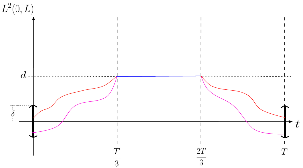
Concerning the construction of solutions to the Theorems 1.4 and 1.5 we follow the following procedure: In the first time, we construct a solution that starts from $y_{0}$ and reaches at time $T/3$ a state which is in some sense close to $d$ (which is yet to be defined). Then we construct a solution (close to the state solution $d$ ), which starts at time $2T/3$ from the previous state. In the last step, we bring the latter state to 0 via a function $y_{2}$ , as we can see in Figure 1 below. For details of this construction see the characterization of the function $y$ in (3.52).

Refer to caption — Figure 1: Solutions driving states close to 0 to constants and vice versa.

We finish this introduction with an outline of this work which consists of four parts, including the introduction. Section 2 gives an overview of the well-posedness of the system (1.9). Section 3 is devoted to proving carefully the controllability of the system (1.9) when $L\in\mathcal{R}_{c}$ . Precisely, in the first part of Section 3, we deal with the proof of Theorem 1.6. In the second part, we prove the construction of the function $y$ mentioned before, and finally, in the third part of Section 3, we use these previous results to achieve Theorem 1.4.

2 Overview of the well-posedness theory

In this section, we review the well-posedness theory for the KdV equation. The results presented here can be found in [5, 7, 21]. For that, consider $L>0$ and $T_{0},T_{1}\in\mathbb{R}$ with $T_{0}<T_{1}$ . We define the space

\displaystyle\mathcal{Z}_{T_{0},T_{1}}:=C\left([T_{0},T_{1}];L^{2}(0,L)\right)\cap L^{2}\left([T_{0},T_{1}];H^{1}(0,L)\right)

which is a Banach space with the following norm

\displaystyle\|y\|_{\mathcal{Z}_{T_{0},T_{1}}}:=\max_{t\in[T_{0},T_{1}]}\|y(\cdot,t)\|_{L^{2}(0,L)}+\left(\int_{T_{0}}^{T_{1}}\|y(\cdot,t)\|_{H^{1}(0,L)}^{2}dt\right)^{1/2}.

For any $T>0$ we denote $\mathcal{Z}_{0,T}$ simply by $\mathcal{Z}_{T}$ .

Additionally, let $T>0$ be given and consider the space

\displaystyle\mathcal{H}_{T}:=H^{-\frac{1}{3}}(0,T)\times L^{2}(0,T)\times H^{-\frac{1}{3}}(0,T)

with a norm

\|(h_{1},h_{2},h_{3})\|_{\mathcal{H}_{T}}:=\|h_{1}\|_{H^{-\frac{1}{3}}(0,T)}+\|h_{2}\|_{L^{2}(0,T)}+\|h_{3}\|_{H^{-\frac{1}{3}}(0,T)}.

The next proposition, showed in [7, Proposition 2.5], provides the well-posedness to the following system

\displaystyle\left\{\begin{array}[]{ll}u_{t}+u_{xxx}=f,&\ \text{ in }(0,L)\times(0,T),\\ u_{xx}(0,t)=h_{1}(t),\ u_{x}(L,t)=h_{2}(t),\ u_{xx}(L,t)=h_{3}(t),&\ \text{ in }(0,T),\\ u(x,0)=u_{0},&\ \text{ in }(0,L).\end{array}\right.

(2.13)

Proposition 2.1 (Caicedo, Capistrano-Filho, Zhang [7]).

For any $v_{0}\in L^{2}(0,L)$ , ${\bf h}=(h_{1},h_{2},h_{3})\in\mathcal{H}_{T}$ and $f\in L^{1}(0,T,L^{2}(0,L))$ , the IBVP (2.13) admits a unique mild solution $u\in\mathcal{Z}_{T}$ , which satisfies

\displaystyle\partial_{x}^{j}u\in L^{\infty}_{x}(0,L;H^{(1-j)/3}(0,T)),\ j=0,1,2.

Moreover, there exists $C_{1}>0$ such that

\displaystyle\|u\|_{\mathcal{Z}_{T}}+\sum_{j=0}^{2}\left\|\partial_{x}^{j}u\right\|_{L^{\infty}_{x}(0,L;H^{(1-j)/3}(0,T))}\leq C_{1}\left(\|u_{0}\|_{L^{2}(0,L)}+\|{\bf h}\|_{\mathcal{H}_{T}}+\|f\|_{L^{1}(0,T;L^{2}(0,L))}\right).

Remark 2.2.

We highlight that the constant $C_{1}$ in the above result depends on $T$ . However, if $\theta\in(0,T]$ then, the estimates in the Proposition 2.1 hold with the same constant $C_{1}$ corresponding to $T$ .

In fact, let $u_{0}\in L^{2}(0,L)$ , ${\bf h}\in\mathcal{H}_{\theta},\ f\in L^{1}(0,\theta;L^{2}(0,L))$ and $u\in\mathcal{Z}_{\theta}$ the solution of (2.13) corresponding to these datas. We extend ${\bf h}$ and $f$ to $[0,T]$ (we will also denote these extensions by ${\bf h}$ and $f$ ) putting

{\bf h}=0\text{ in }(\theta,T]\quad\text{and}\quad f=0\text{ in }(\theta,T].

Now, denote by $\tilde{u}\in\mathcal{Z}_{T}$ the corresponding solution of (2.13). Then, from Proposition 2.1, we have $\tilde{u}\big{|}_{[0,\theta]}=u$ and

	$\displaystyle\\|u\\|_{\mathcal{Z}_{\theta}}\leq\\|\tilde{u}\\|_{\mathcal{Z}_{T}}$	$\displaystyle\leq C_{1}\left(\\|u_{0}\\|_{L^{2}(0,L)}+\\|{\bf h}\\|_{\mathcal{H}_{T}}+\\|f\\|_{L^{1}(0,T;L^{2}(0,L))}\right)$
		$\displaystyle=C_{1}\left(\\|u_{0}\\|_{L^{2}(0,L)}+\\|{\bf h}\\|_{\mathcal{H}_{\theta}}+\\|f\\|_{L^{1}(0,\theta;L^{2}(0,L))}\right).$

Using the Proposition 2.1 we can get properties for the linear problem

\displaystyle\left\{\begin{array}[]{ll}y_{t}+(ay)_{x}+y_{xxx}=f,&\ \text{ in }(0,L)\times(0,T),\\ y_{xx}(0,t)=h_{1}(t),\ y_{x}(L,t)=h_{2}(t),\ y_{xx}(L,t)=h_{3}(t),&\ \text{ in }(0,T),\\ y(x,0)=y_{0}(x),&\ \text{ in }(0,L),\end{array}\right.

(2.17)

where $a\in\mathcal{Z}_{T}$ is given. To do this, the following lemma will be very useful and was proved in [22, Lemma 3].

Lemma 2.3 (Kramer, Zhang [22]).

There exists a constant $C>0$ such that

\displaystyle\int_{0}^{T}\|uv_{x}(\cdot,t)\|_{L^{2}(0,L)}dt\leq C\left(T^{\frac{1}{2}}+T^{\frac{1}{3}}\right)\|u\|_{\mathcal{Z}_{T}}\|v\|_{\mathcal{Z}_{T}},

for every $u,v\in\mathcal{Z}_{T}$ .

With these previous results in hand, the following proposition gives us the well-posedness to the general system (2.17), which will be used several times so, for the sake of completeness, we will give the proof.

Proposition 2.4.

For any $y_{0}\in L^{2}(0,L)$ , ${\bf h}=(h_{1},h_{2},h_{3})\in\mathcal{H}_{T}$ and $f\in L^{1}(0,T,L^{2}(0,L))$ , the IBVP (2.17) admits a unique mild solution $y\in\mathcal{Z}_{T}$ , which satisfies

\displaystyle\partial_{x}^{j}y\in L^{\infty}_{x}(0,L;H^{(1-j)/3}(0,T)),\ j=0,1,2,

and

\displaystyle\|y\|_{\mathcal{Z}_{T}}\leq C_{2}\left(\|y_{0}\|_{L^{2}(0,L)}+\|{\bf h}\|_{\mathcal{H}_{T}}+\|f\|_{L^{1}(0,T;L^{2}(0,L))}\right),

for some positive constant $C_{2}$ which depends only on $T$ and $\|a\|_{\mathcal{Z}_{T}}$ . In addition, the solution $y$ possesses the following sharp trace estimates

\displaystyle\sum_{j=0}^{2}\left\|\partial_{x}^{j}y\right\|_{L^{\infty}_{x}(0,L;H^{(1-j)/3}(0,T))}\leq C_{2}\left(\|y_{0}\|_{L^{2}(0,L)}+\|{\bf h}\|_{\mathcal{H}_{T}}+\|f\|_{L^{1}(0,T;L^{2}(0,L))}\right).

In particular, the map $(y_{0},{\bf h},f)\mapsto y$ is Lipschitz continuous.

Proof 2.5.

Let $y_{0}\in L^{2}(0,L)$ , ${\bf h}\in\mathcal{H}_{T}$ and $f\in L^{1}(0,T;L^{2}(0,L))$ be given. Consider $\theta$ satisfying $0<\theta\leq T$ and define the map $\Gamma:\mathcal{Z}_{\theta}\rightarrow\mathcal{Z}_{\theta}$ in the next way: for $y\in\mathcal{Z}_{\theta}$ , put $\Gamma y$ being the solution of

\displaystyle\left\{\begin{array}[]{ll}u_{t}+u_{xxx}=f-(ay)_{x},&\ \text{ in }(0,L)\times(0,\theta),\\ u_{xx}(0,t)=h_{1}(t),\ u_{x}(L,t)=h_{2}(t),\ u_{xx}(L,t)=h_{3}(t),&\ \text{ in }(0,\theta),\\ u(x,0)=y_{0}(x),&\ \text{ in }(0,L).\end{array}\right.

Consider the set

\displaystyle B=\left\{y\in\mathcal{Z}_{\theta};\ \|y\|_{\mathcal{Z}_{\theta}}\leq r\right\},

with $r>0$ to be determined later. From Proposition 2.1 and Lemma 2.3 we have for any $y\in B$ the following estimate

$\displaystyle\\|\Gamma y\\|_{\mathcal{Z}_{\theta}}\leq$	$\displaystyle C_{1}\left(\\|y_{0}\\|_{L^{2}(0,L)}+\\|{\bf h}\\|_{\mathcal{H}_{\theta}}+\\|f\\|_{L^{1}(0,\theta;L^{2}(0,L))}+\\|(ay)_{x}\\|_{L^{1}(0,\theta;L^{2}(0,L))}\right)$	(2.18)
$\displaystyle\leq$	$\displaystyle C_{1}\left(\\|y_{0}\\|_{L^{2}(0,L)}+\\|{\bf h}\\|_{\mathcal{H}_{\theta}}+\\|f\\|_{L^{1}(0,\theta;L^{2}(0,L))}\right)$
	$\displaystyle+2C_{1}C\left(\theta^{\frac{1}{2}}+\theta^{\frac{1}{3}}\right)\\|a\\|_{\mathcal{Z}_{\theta}}\\|y\\|_{\mathcal{Z}_{\theta}}$
$\displaystyle\leq$	$\displaystyle C_{1}\left(\\|y_{0}\\|_{L^{2}(0,L)}+\\|{\bf h}\\|_{\mathcal{H}_{\theta}}+\\|f\\|_{L^{1}(0,\theta;L^{2}(0,L))}\right)$
	$\displaystyle+2C_{1}C\left(\theta^{\frac{1}{2}}+\theta^{\frac{1}{3}}\right)\\|a\\|_{\mathcal{Z}_{T}}\\|y\\|_{\mathcal{Z}_{\theta}}.$

Choosing

r=2C_{1}\left(\|y_{0}\|_{L^{2}(0,L)}+\|{\bf h}\|_{\mathcal{H}_{\theta}}+\|f\|_{L^{1}(0,\theta;L^{2}(0,L))}\right)

and $\theta$ satisfying

\displaystyle 2C_{1}C\left(\theta^{\frac{1}{2}}+\theta^{\frac{1}{3}}\right)\|a\|_{\mathcal{Z}_{T}}<\frac{1}{2},

(2.19)

the inequality (2.18) give us

\displaystyle\|\Gamma y\|_{\mathcal{Z}_{\theta}}\leq\frac{r}{2}+\frac{r}{2}=r,

that is, $\Gamma(B)\subset B$ . Furthermore, $\Gamma y-\Gamma w$ solves

\displaystyle\left\{\begin{array}[]{ll}u_{t}+u_{xxx}=[a(-y+w)]_{x},&\ \text{ in }(0,L)\times(0,\theta),\\ u_{xx}(0,t)=u_{x}(L,t)=u_{xx}(L,t)=0,&\ \text{ in }(0,\theta),\\ u(x,0)=0,&\ \text{ in }(0,L).\end{array}\right.

So, from Proposition 2.1, Lemma 2.3 and inequality (2.19), we have

	$\displaystyle\\|\Gamma y-\Gamma w\\|_{\mathcal{Z}_{\theta}}$	$\displaystyle\leq C_{1}\\|[a(y-w)]_{x}\\|_{L^{1}(0,\theta;L^{2}(0,L))}$
		$\displaystyle\leq 2C_{1}C\left(\theta^{\frac{1}{2}}+\theta^{\frac{1}{3}}\right)\\|a\\|_{\mathcal{Z}_{\theta}}\\|y-w\\|_{\mathcal{Z}_{\theta}}$
		$\displaystyle\leq 2C_{1}C\left(\theta^{\frac{1}{2}}+\theta^{\frac{1}{3}}\right)\\|a\\|_{\mathcal{Z}_{T}}\\|y-w\\|_{\mathcal{Z}_{\theta}}$
		$\displaystyle<\frac{1}{2}\\|y-w\\|_{\mathcal{Z}_{\theta}}.$

Thus, $\Gamma:B\rightarrow B$ is a contraction so that, by Banach’s fixed point theorem, $\Gamma$ has a fixed point $y\in B$ which is a solution to the problem (2.17) in $[0,\theta]$ , corresponding to data $(y_{0},{\bf h},f)$ . Additionally, inequalities (2.18) and (2.19) yields that

\displaystyle\|y\|_{\mathcal{Z}_{\theta}}\leq C_{1}\left(\|y_{0}\|_{L^{2}(0,L)}+\|{\bf h}\|_{\mathcal{H}_{\theta}}+\|f\|_{L^{1}(0,\theta;L^{2}(0,L))}\right)+\frac{1}{2}\|y\|_{\mathcal{Z}_{\theta}}

and, therefore,

\displaystyle\|y\|_{\mathcal{Z}_{\theta}}\leq 2C_{1}\left(\|y_{0}\|_{L^{2}(0,L)}+\|{\bf h}\|_{\mathcal{H}_{\theta}}+\|f\|_{L^{1}(0,\theta;L^{2}(0,L))}\right).

Since $\theta$ depends only on $a$ , with a standard continuation extension argument, the solution $y$ can be extended to interval $[0,T]$ and the following estimate holds

\displaystyle\|y\|_{\mathcal{Z}_{T}}\leq C_{2}\left(\|y_{0}\|_{L^{2}(0,L)}+\|{\bf h}\|_{\mathcal{H}_{T}}+\|f\|_{L^{1}(0,T;L^{2}(0,L))}\right),

(2.20)

for some suitable constant $C_{2}>0$ which only depends on $T$ and $\|a\|_{\mathcal{Z}_{T}}$ . Therefore, it follows from (2.20) that the map $(y_{0},{\bf h},f)\mapsto y$ is Lipschitz continuous and, as a consequence of this, we have the uniqueness of the solution $y$ in $\mathcal{Z}_{T}$ . The sharp trace estimates follow as a consequence of the Proposition 2.1, showing the proposition.

Now, we will study the well-posedness of the nonlinear problem, namely:

\displaystyle\left\{\begin{array}[]{ll}y_{t}+(ay)_{x}+y_{xxx}+yy_{x}=f,&\ \text{ in }(0,L)\times(0,T),\\ y_{xx}(0,t)=h_{1}(t),\ y_{x}(L,t)=h_{2}(t),\ y_{xx}(L,t)=h_{3}(t),&\ \text{ in }(0,T),\\ y(x,0)=y_{0}(x),&\ \text{ in }(0,L).\end{array}\right.

(2.24)

The result can be read as follows.

Proposition 2.6.

Let $a\in\mathcal{Z}_{T}$ be given. For every $y_{0}\in L^{2}(0,L)$ , ${\bf h}=(h_{1},h_{2},h_{3})\in\mathcal{H}_{T}$ and $f\in L^{1}(0,T,L^{2}(0,L))$ there exists a unique mild solution $y\in\mathcal{Z}_{T}$ of (2.24) which satisfies

\|y\|_{\mathcal{Z}_{T}}\leq C_{3}\left(\|y_{0}\|_{L^{2}(0,L)}+\|{\bf h}\|_{L^{2}(0,T)}+\|f\|_{L^{1}(0,T;L^{2}(0,L))}\right)

and

	$\displaystyle\sum_{j=0}^{2}\left\\|\partial_{x}^{j}y\right\\|_{L^{\infty}_{x}(0,L;H^{(1-j)/3}(0,T))}\leq$	$\displaystyle C_{3}\left(\\|y_{0}\\|_{L^{2}(0,L)}+\\|h\\|_{L^{2}(0,T)}~{}+\\|f\\|_{L^{1}(0,T;L^{2}(0,L))}\right)$
		$\displaystyle+C_{3}\left(\\|y_{0}\\|_{L^{2}(0,L)}+\\|h\\|_{L^{2}(0,T)}+\\|f\\|_{L^{1}(0,T;L^{2}(0,L))}\right)^{2},$

for some constant $C_{3}>0$ . Furthermore, the corresponding solution map $S$ is locally Lipschitz continuous, that is, given $\lambda>0$ there exist $L_{\lambda}>0$ such that, for every

(y_{0},{\bf h},f_{0}),(y_{1},{\bf g},f_{1})\in L^{2}(0,L)\times\mathcal{H}_{T}\times L^{1}(0,T;L^{2}(0,L))

with

	$\displaystyle\\|y_{0}\\|_{L^{2}(0,L)}+\\|{\bf h}\\|_{\mathcal{H}_{T}}+\\|f_{0}\\|_{L^{1}(0,T;L^{2}(0,L))}<\lambda,$
	$\displaystyle\\|y_{1}\\|_{L^{2}(0,L)}+\\|{\bf g}\\|_{\mathcal{H}_{T}}+\\|f_{1}\\|_{L^{1}(0,T;L^{2}(0,L))}<\lambda,$

we have

\begin{split}\|S(y_{0},{\bf h},f_{0})-S(y_{1},{\bf g},f_{1})\|_{\mathcal{Z}_{T}}\leq&L_{\lambda}\left(\|y_{0}-y_{1}\|_{L^{2}(0,L)}\right.\\ &\left.+\|{\bf h}-{\bf g}\|_{\mathcal{H}_{T}}+\|f_{0}-f_{1}\|_{L^{1}(0,T;L^{2}(0,L))}\right).\end{split}

Proof 2.7.

We will proceed as follows: First, we will show the existence of a solution and obtain the desired estimates. Secondly, we will get an estimate that provides the uniqueness of the solution and guarantees that $S$ is locally Lipschitz continuous.

To do that, consider $y_{0}\in L^{2}(0,L)$ , ${\bf h}\in\mathcal{H}_{T}$ and $f\in L^{1}(0,T;L^{2}(0,L))$ . Let $\theta$ satisfying $0<\theta\leq T$ and define the map $\Gamma:\mathcal{Z}_{\theta}\rightarrow\mathcal{Z}_{\theta}$ in the following way: For $y\in\mathcal{Z}_{\theta}$ , pick $\Gamma y$ as solution of the following problem

\displaystyle\left\{\begin{array}[]{ll}u_{t}+(au)_{x}+u_{xxx}=f-yy_{x},&\ \text{ in }(0,L)\times(0,\theta),\\ u_{xx}(0,t)=h_{1}(t),\ u_{x}(L,t)=h_{2}(t),\ u_{xx}(L,t)=h_{3}(t),&\ \text{ in }(0,\theta),\\ u(x,0)=y_{0}(x),&\ \text{ in }(0,L).\end{array}\right.

Consider the set

\displaystyle B=\left\{y\in\mathcal{Z}_{\theta};\ \|y\|_{\mathcal{Z}_{\theta}}\leq r\right\},

with $r>0$ to be determined later. Using Proposition 2.4 and Lemma 2.3 we obtain, for any $y\in B$ ,

	$\displaystyle\\|\Gamma y\\|_{\mathcal{Z}_{\theta}}$	$\displaystyle\leq C_{2}\left(\\|y_{0}\\|_{L^{2}(0,L)}+\\|{\bf h}\\|_{\mathcal{H}_{\theta}}+\\|f\\|_{L^{1}(0,\theta;L^{2}(0,L))}+\\|yy_{x}\\|_{L^{1}(0,\theta;L^{2}(0,L))}\right)$		(2.25)
		$\displaystyle\leq C_{2}\left(\\|y_{0}\\|_{L^{2}(0,L)}+\\|{\bf h}\\|_{\mathcal{H}_{\theta}}+\\|f\\|_{L^{1}(0,\theta;L^{2}(0,L))}\right)+C_{2}C\left(\theta^{\frac{1}{2}}+\theta^{\frac{1}{3}}\right)\\|y\\|_{\mathcal{Z}_{T}}^{2}.$		(2.25)

Choosing

\displaystyle r=4C_{2}\left(\|y_{0}\|_{L^{2}(0,L)}+\|{\bf h}\|_{\mathcal{H}_{\theta}}+\|f\|_{L^{1}(0,\theta;L^{2}(0,L))}\right)

and $\theta$ satisfying

\displaystyle C_{2}C\left(\theta^{\frac{1}{2}}+\theta^{\frac{1}{3}}\right)r<\frac{1}{4},

(2.26)

inequality (2.25) give us

\displaystyle\|\Gamma\|_{\mathcal{Z}_{T}}

\displaystyle\leq\frac{r}{4}+\frac{r}{4}=\frac{r}{2}<r,

that is, $\Gamma(B)\subset B$ . Moreover given $y,w\in B$ , $\Gamma y-\Gamma w$ solves

\displaystyle\left\{\begin{array}[]{ll}u_{t}+(au)_{x}+u_{xxx}=-yy_{x}+ww_{x},&\ \text{ in }(0,L)\times(0,\theta),\\ u_{xx}(0,t)=0,\ u_{x}(L,t)=0,\ u_{xx}(L,t)=0,&\ \text{ in }(0,\theta),\\ u(x,0)=0,&\ \text{ in }(0,L).\end{array}\right.

Therefore, from Proposition 2.4,

\displaystyle\|\Gamma y-\Gamma w\|_{\mathcal{Z}_{\theta}}\leq C_{2}\|yy_{x}-ww_{x}\|_{L^{1}(0,\theta;L^{2}(0,L))}.

Note that

\displaystyle yy_{x}-ww_{x}=\frac{1}{2}\big{[}(y+w)_{x}(y-w)+(y+w)(y-w)_{x}\big{]}.

Then, thanks to the Lemma 2.3, we get that

	$\displaystyle\\|yy_{x}-ww_{x}\\|_{L^{1}(0,\theta;L^{2}(0,L))}$
	$\displaystyle\leq\frac{1}{2}\big{[}\\|(y+w)_{x}(y-w)\\|_{L^{1}(0,\theta;L^{2}(0,L))}+\\|(y+w)(y-w)_{x}\\|_{L^{1}(0,\theta;L^{2}(0,L))}\big{]}$
	$\displaystyle\leq\frac{1}{2}\left[C\left(\theta^{\frac{1}{2}}+\theta^{\frac{1}{3}}\right)\\|y+w\\|_{\mathcal{Z}_{\theta}}\\|y-w\\|_{\mathcal{Z}_{\theta}}+C\left(\theta^{\frac{1}{2}}+\theta^{\frac{1}{3}}\right)\\|y+w\\|_{\mathcal{Z}_{\theta}}\\|y-w\\|_{\mathcal{Z}_{\theta}}\right]$
	$\displaystyle=C\left(\theta^{\frac{1}{2}}+\theta^{\frac{1}{3}}\right)\\|y+w\\|_{\mathcal{Z}_{\theta}}\\|y-w\\|_{\mathcal{Z}_{\theta}}$
	$\displaystyle\leq 2C\left(\theta^{\frac{1}{2}}+\theta^{\frac{1}{3}}\right)r\\|y-w\\|_{\mathcal{Z}_{\theta}}$

and, using (2.26) yields

\displaystyle\|\Gamma y-\Gamma w\|_{\mathcal{Z}_{\theta}}\leq 2C_{2}C\left(\theta^{\frac{1}{2}}+\theta^{\frac{1}{3}}\right)r\|y-w\|_{\mathcal{Z}_{\theta}}<\frac{1}{2}\|y-w\|_{\mathcal{Z}_{\theta}}.

Hence, $\Gamma:B\rightarrow B$ is a contraction so that, by Banach’s fixed point theorem, $\Gamma$ has a fixed point $y\in B$ which is a solution to the problem (2.24) in $[0,\theta]$ , corresponding to data $(y_{0},{\bf h},f)$ .

Furthermore, due to the inequalities (2.25) and (2.26), we have

\displaystyle\|y\|_{\mathcal{Z}_{\theta}}\leq C_{2}\left(\|y_{0}\|_{L^{2}(0,L)}+\|{\bf h}\|_{\mathcal{H}_{\theta}}+\|f\|_{L^{1}(0,\theta;L^{2}(0,L))}\right)+\frac{1}{4}\|y\|_{\mathcal{Z}_{\theta}},

and, therefore

\displaystyle\|y\|_{\mathcal{Z}_{\theta}}\leq\frac{4}{3}C_{2}\left(\|y_{0}\|_{L^{2}(0,L)}+\|{\bf h}\|_{\mathcal{H}_{\theta}}+\|f\|_{L^{1}(0,\theta;L^{2}(0,L))}\right).

Since $\theta$ depends only on $a$ , with a standard continuation extension argument, the solution $y$ can be extended to interval $[0,T]$ and the following estimate holds

\displaystyle\|y\|_{\mathcal{Z}_{T}}\leq\tilde{C}_{3}\left(\|y_{0}\|_{L^{2}(0,L)}+\|{\bf h}\|_{\mathcal{H}_{T}}+\|f\|_{L^{1}(0,T;L^{2}(0,L))}\right),

(2.27)

for some suitable constant $\tilde{C}_{3}>0$ which only depends on $T$ and $a$ . Now, using one more time the Proposition 2.6 together with Lemma 2.3 we obtain

	$\displaystyle\sum_{j=0}^{2}\left\\|\partial_{x}^{j}y\right\\|_{L^{\infty}_{x}(0,L;H^{(1-j)/3}(0,T))}$
	$\displaystyle\leq C_{2}\left(\\|y_{0}\\|_{L^{2}(0,L)}+\\|{\bf h}\\|_{\mathcal{H}_{T}}+\\|f\\|_{L^{1}(0,T;L^{2}(0,L))}+\\|yy_{x}\\|_{L^{1}(0,T;L^{2}(0,L))}\right)$
	$\displaystyle\leq C_{2}\left(\\|y_{0}\\|_{L^{2}(0,L)}+\\|{\bf h}\\|_{\mathcal{H}_{T}}+\\|f\\|_{L^{1}(0,T;L^{2}(0,L))}\right)+C_{2}C\left(\theta^{\frac{1}{2}}+\theta^{\frac{1}{3}}\right)\\|y\\|_{\mathcal{Z}_{T}}^{2}.$

By (2.27) it follows that

	$\displaystyle\sum_{j=0}^{2}\left\\|\partial_{x}^{j}y\right\\|_{L^{\infty}_{x}(0,L;H^{(1-j)/3}(0,T))}$
	$\displaystyle\leq C_{2}\left(\\|y_{0}\\|_{L^{2}(0,L)}+\\|{\bf h}\\|_{\mathcal{H}_{T}}+\\|f\\|_{L^{1}(0,T;L^{2}(0,L))}\right)$
	$\displaystyle+C_{2}C\left(\theta^{\frac{1}{2}}+\theta^{\frac{1}{3}}\right)\tilde{C}^{2}\left(\\|y_{0}\\|_{L^{2}(0,L)}+\\|{\bf h}\\|_{\mathcal{H}_{T}}+\\|f\\|_{L^{1}(0,T;L^{2}(0,L))}\right)^{2}.$

Choosing

\displaystyle C_{3}:=\max\left\{\tilde{C}_{3},C_{2},C_{2}C\left(\theta^{\frac{1}{2}}+\theta^{\frac{1}{3}}\right)\tilde{C}^{2}\right\}

we obtain the desired estimates.

Now, consider

(y_{0},{\bf h},f_{0}),(y_{1},{\bf g},f_{1})\in L^{2}(0,L)\times\mathcal{H}_{T}\times L^{1}(0,T;L^{2}(0,L))

with

	$\displaystyle\\|y_{0}\\|_{L^{2}(0,L)}+\\|{\bf h}\\|_{\mathcal{H}_{T}}+\\|f_{0}\\|_{L^{1}(0,T;L^{2}(0,L))}<\lambda,$
	$\displaystyle\\|y_{1}\\|_{L^{2}(0,L)}+\\|{\bf g}\\|_{\mathcal{H}_{T}}+\\|f_{1}\\|_{L^{1}(0,T;L^{2}(0,L))}<\lambda.$

Write ${\bf h}=(h_{1},h_{2},h_{3})$ and ${\bf g}=(g_{1},g_{2},g_{3})$ . Let $y$ and $u$ be solutions of

\displaystyle\left\{\begin{array}[]{ll}y_{t}+(ay)_{x}+y_{xxx}+yy_{x}=f_{0},&\ \text{ in }(0,L)\times(0,T),\\ y_{xx}(0,t)=h_{1}(t),\ y_{x}(L,t)=h_{2}(t),\ y_{xx}(L,t)=h_{3}(t),&\ \text{ in }(0,T),\\ y(x,0)=y_{0}(x)&\ \text{ in }(0,L),\end{array}\right.

and

\displaystyle\left\{\begin{array}[]{ll}u_{t}+(au)_{x}+u_{xxx}+uu_{x}=f_{1},&\ \text{ in }(0,L)\times(0,T),\\ u_{xx}(0,t)=g_{1}(t),\ u_{x}(L,t)=g_{2}(t),\ u_{xx}(L,t)=g_{3}(t),&\ \text{ in }(0,T),\\ u(x,0)=y_{1}(x)&\ \text{ in }(0,L),\end{array}\right.

respectively. Then, $w=y-u$ solves the problem

\displaystyle\left\{\begin{array}[]{ll}w_{t}+\big{[}\left(a+\frac{1}{2}(y+u)\right)w\big{]}_{x}+w_{xxx}=f_{0}-f_{1},&\ \text{ in }(0,L)\times(0,T,)\\ w_{xx}(0,\cdot)=h_{1}-g_{1},\ w_{x}(L,\cdot)=h_{2}-g_{2},\ w_{xx}(L,\cdot)=h_{3}-g_{3},&\ \text{ in }(0,T),\\ w(x,0)=y_{0}(x)-y_{1}(x),&\ \text{ in }(0,L).\end{array}\right.

From Proposition 2.4 it follows that

\displaystyle\|y-u\|_{\mathcal{Z}_{T}}\leq D\left(\|y_{0}-y_{1}\|_{L^{2}(0,L)}+\|{\bf h}-{\bf g}\|_{\mathcal{H}_{T}}+\|f_{0}-f_{1}\|_{L^{1}(0,T;L^{2}(0,L))}\right),

(2.28)

where $D$ is a constant which depends on $T$ and $\|a+\frac{1}{2}(y+u)\|_{\mathcal{Z}_{T}}$ . But, using (2.27) we have

	$\displaystyle\\|a+\frac{1}{2}(y+u)\\|_{\mathcal{Z}_{T}}\leq$	$\displaystyle\\|a\\|_{\mathcal{Z}_{T}}+\frac{1}{2}\left(\\|y\\|_{\mathcal{Z}_{T}}+\\|u\\|_{\mathcal{Z}_{T}}\right)$
	$\displaystyle\leq$	$\displaystyle\\|a\\|_{\mathcal{Z}_{T}}+\frac{\tilde{C}_{3}}{2}\left(\\|y_{0}\\|_{L^{2}(0,L)}+\\|{\bf h}\\|_{\mathcal{H}_{T}}+\\|f_{0}\\|_{L^{1}(0,T;L^{2}(0,L))}\right)$
		$\displaystyle+\frac{\tilde{C}_{3}}{2}\left(\\|y_{1}\\|_{L^{2}(0,L)}+\\|{\bf g}\\|_{\mathcal{H}_{T}}+\\|f_{1}\\|_{L^{1}(0,T;L^{2}(0,L))}\right)$

and, consequently,

\displaystyle\|a+\frac{1}{2}(y+u)\|_{\mathcal{Z}_{T}}

\displaystyle\leq\|a\|_{\mathcal{Z}_{T}}+\tilde{C}_{3}\lambda.

Hence, the constant $D$ can be chosen depending only on $T$ and $\|a\|_{\mathcal{Z}_{T}}$ (and also on $\lambda$ ), so that, (2.28) gives us the uniqueness of the solution which turns the solution map $S$ well-defined. Moreover, from (2.28)

\begin{split}\|S(y_{0},{\bf h},f_{0})-S(y_{1},{\bf g},f_{1})\|_{\mathcal{Z}_{T}}\leq&D\left(\|y_{0}-y_{1}\|_{L^{2}(0,L)}\right.\\ &\left.+\|{\bf h}-{\bf g}\|_{\mathcal{H}_{T}}+\|f_{0}-f_{1}\|_{L^{1}(0,T;L^{2}(0,L))}\right),\end{split}

which concludes the proof.

Finally, the following Lemma, whose proof can be found in [24], will be useful in the next section.

Lemma 2.8 (Rosier [24]).

If $y\in\mathcal{Z}_{T}$ then $yy_{x}\in L^{1}(0,T;L^{2}(0,L))$ and the map

\displaystyle\begin{array}[]{rcl}\mathcal{Z}_{T}&\longrightarrow&L^{1}(0,T;L^{2}(0,L))\\ y&\longmapsto&yy_{x},\end{array}

is continuous. More precisely, for every $y,z\in\mathcal{Z}_{T}$ we have that

\begin{split}\|yy_{x}-zz_{x}\|_{L^{1}(0,T;L^{2}(0,L))}\leq&C_{4}\left(\|y\|_{L^{2}(0,T;H^{1}(0,L))}\right.\\ &\left.+\|z\|_{L^{2}(0,T;H^{1}(0,L))}\right)\|y-z\|_{L^{2}(0,T;H^{1}(0,L))},\end{split}

where $C_{4}$ is a positive constant that depends only on $L$ .

Remark 2.9.

We end this subsection with the following remarks.

1.

For every $a\in\mathcal{Z}_{T}$ , the Proposition 2.4 give us the well-definition for the solution operator

$\Lambda_{a}:L^{2}(0,L)\times\mathcal{H}_{T}\times L^{1}(0,T;L^{2}(0,L))\rightarrow\mathcal{Z}_{T}$

where, for each $(y_{0},{\bf h},f)\in L^{2}(0,L)\times\mathcal{H}_{T}\times L^{1}(0,T;L^{2}(0,L))$ , $\Lambda_{a}(y_{0},{\bf h},f)$ is the corresponding solution to the problem (2.17). Furthermore, the Proposition 2.6 guarantees that $\Lambda_{a}$ is a bounded linear operator.
2.

Of course, the constant $C_{2}>0$ in the Proposition 2.4 depends on $\|a\|_{\mathcal{Z}_{T}}$ . However, given $M>0$ , the same constant $C_{2}$ can be used for every $a\in\mathcal{Z}_{T}$ with $\|a\|_{\mathcal{Z}_{T}}\leq M$ .

3 Boundary controllability in the critical lenght

In this section, we study the controllability of the system

\displaystyle\left\{\begin{array}[]{ll}y_{t}+y_{x}+y_{xxx}+yy_{x}=0,&\ \text{ in }(0,L)\times(0,T),\\ y_{xx}(0,t)=0,\ y_{x}(L,t)=h(t),\ y_{xx}(L,t)=0,&\ \text{ in }(0,T),\\ y(x,0)=y_{0}(x)&\ \text{ in }(0,L),\end{array}\right.

(3.32)

when $L$ is a critical length. We will use the return method together with the fixed point argument to ensure the controllability of the system (3.32) when $L\in\mathcal{R}_{c}$ . Before presenting the proof of the main result, let us give a preliminary result which is important in our analysis.

3.1 An auxiliary result

Given $c\neq-1$ , the set of critical lengths for the linearization of (3.32) around $c$ is

\displaystyle\mathcal{R}_{c}:=\left\{\frac{2\pi}{\sqrt{3(c+1)}}\sqrt{m^{2}+ml+l^{2}}\ ;\ m,l\in\mathbb{N}^{*}\right\}\cup\left\{\frac{m\pi}{\sqrt{c+1}};\ m\in\mathbb{N}^{*}\right\}.

As mentioned before, when $L\in\mathcal{R}_{c}$ , the linear system

\displaystyle\left\{\begin{array}[]{lll}y_{t}+(1+c)y_{x}+y_{xxx}=0,&\text{ in }(0,L)\times(0,T),\\ y_{xx}(0,t)=0,\ y_{x}(L,t)=h(t),\ y_{xx}(L,t)=0,&\text{ in }(0,T),\\ y(x,0)=y_{0}(x),&\text{ in }(0,L),\end{array}\right.

(3.36)

is not exactly controllable. So, in this section, we first give the proof of Theorem 1.6.

Proof 3.1.

(Proof of Theorem 1.6.) We will split the proof into two cases.

First case: $L=2\pi\frac{\sqrt{j^{2}+jk+k^{2}}}{\sqrt{3(c+1)}}$ for some $(j,k)\in\mathbb{N}^{*}\times\mathbb{N}^{*}$ .

Let $d\neq-1$ and suppose that $L\in\mathcal{R}_{d}$ . Then

L=2\pi\frac{\sqrt{m^{2}+ml+l^{2}}}{\sqrt{3(d+1)}};\ m,l\in\mathbb{N}^{*}

(3.37)

L=\frac{m\pi}{\sqrt{d+1}};\ m\in\mathbb{N}^{*}.

(3.38)

If (3.37) is the case, we have that

2\pi\frac{\sqrt{j^{2}+jk+k^{2}}}{\sqrt{3(c+1)}}=2\pi\frac{\sqrt{m^{2}+ml+l^{2}}}{\sqrt{3(d+1)}},

which implies

d=\frac{(c+1)(m^{2}+ml+l^{2})}{j^{2}+jk+k^{2}}-1

with $m,l\in\mathbb{N}^{*}$ .

Otherwise, if (3.38) holds, so

2\pi\frac{\sqrt{j^{2}+jk+k^{2}}}{\sqrt{3(c+1)}}=\frac{m\pi}{\sqrt{d+1}}

giving that

d=\frac{3m^{2}(c+1)}{4(j^{2}+jk+k^{2})}-1

where $m\in\mathbb{N}^{*}$ . Therefore, if $L\in\mathcal{R}_{d}$ then we necessarily have $d\in\mathcal{A}_{1}\cup\mathcal{B}_{1}$ . Here,

\mathcal{A}_{1}:=\left\{\frac{(c+1)(m^{2}+ml+l^{2})}{j^{2}+jk+k^{2}}-1,\ m,l\in\mathbb{N}^{*}\right\}

and

\mathcal{B}_{1}:=\left\{\frac{3m^{2}(c+1)}{4(j^{2}+jk+k^{2})}-1;\ m\in\mathbb{N}^{*}\right\}.

We are now in a position to prove that $\mathcal{A}_{1}\cup\mathcal{B}_{1}$ is discrete. To do that, consider $x,y\in\mathcal{A}_{1}$ such that $x\neq y$ in the form

x=\frac{(c+1)(m_{1}^{2}+m_{1}l_{1}+l_{1}^{2})}{j^{2}+jk+k^{2}}-1

and

y=\frac{(c+1)(m_{2}^{2}+m_{2}l_{2}+l_{2}^{2})}{j^{2}+jk+k^{2}}-1,

with $m_{1},l_{1},m_{2},l_{2}\in\mathbb{N}^{*}$ . Note that

x-y=\frac{c+1}{j^{2}+jk+k^{2}}\left[(m_{1}^{2}+m_{1}l_{1}+l_{1}^{2})-(m_{2}^{2}+m_{2}l_{2}+l_{2}^{2})\right].

Since $x\neq y$ we have

(m_{1}^{2}+m_{1}l_{1}+l_{1}^{2})\neq(m_{2}^{2}+m_{2}l_{2}+l_{2}^{2}).

Thus

\left|(m_{1}^{2}+m_{1}l_{1}+l_{1}^{2})-(m_{2}^{2}+m_{2}l_{2}+l_{2}^{2})\right|\geq 1

so that

d(x,y)\geq\frac{c+1}{j^{2}+jk+k^{2}},\ \forall x,y\in\mathcal{A}_{1},\ x\neq y.

Analogously, we get

d(x,y)\geq\frac{3(c+1)}{4(j^{2}+jk+k^{2})},\ \forall\ x,y\in\mathcal{B}_{1},x\neq y.

Now, let $x\in\mathcal{A}_{1}$ and $y\in\mathcal{B}_{1}$ with $x\neq y$ , as follow:

x=\frac{(c+1)(m^{2}+ml+l^{2})}{j^{2}+jk+k^{2}}-1

and

y=\frac{3p^{2}(c+1)}{4(j^{2}+jk+k^{2})}-1,

where $m,l,p\in\mathbb{N}^{*}$ . Observe that

\begin{split}x-y=&\frac{(c+1)(m^{2}+ml+l^{2})}{j^{2}+jk+k^{2}}-\frac{3p^{2}(c+1)}{4(j^{2}+jk+k^{2})}\\ =&\frac{4(c+1)(m^{2}+ml+l^{2})}{4(j^{2}+jk+k^{2})}-\frac{3p^{2}(c+1)}{4(j^{2}+jk+k^{2})}\\ =&\frac{c+1}{4(j^{2}+jk+k^{2})}\left[4(m^{2}+ml+l^{2})-3p^{2}\right].\end{split}

Since $x\neq y$ we have that $4(m^{2}+ml+l^{2})$ and $3p^{2}$ are distinct natural numbers so

\left|4(m^{2}+ml+l^{2})-3p^{2}\right|\geq 1

and, consequently, we have

d(x,y)\geq\frac{c+1}{4(j^{2}+jk+k^{2})}.

From all the above we conclude that

d(x,y)\geq\frac{c+1}{4(j^{2}+jk+k^{2})},\ \forall\ x,y\in\mathcal{A}_{1}\cup\mathcal{B}_{1},\ x\neq y,

which implies that $\mathcal{A}_{1}\cup\mathcal{B}_{1}$ is discrete.

Note that $c\in\mathcal{A}_{1}\cup\mathcal{B}_{1}$ since

c=\left[\frac{(c+1)(j^{2}+jk+k^{2})}{j^{2}+jk+k^{2}}-1\right]\in\mathcal{A}_{1}.

As any point in $\mathcal{A}_{1}\cup\mathcal{B}_{1}$ is isolated, there exists $\epsilon_{1}>0$ such that

(c-\epsilon_{1},c+\epsilon_{1})\cap\left[\mathcal{A}_{1}\cup\mathcal{B}_{1}\right]=\{c\}.

Therefore for $d\in(c-\epsilon_{1},c+\epsilon_{1})\backslash\{c\}$ we have that $d\notin\mathcal{A}_{1}\cup\mathcal{B}_{1}$ and, therefore, $L\notin\mathcal{R}_{d}$ .

Second case: $L=\frac{k\pi}{\sqrt{c+1}}$ for some $k\in\mathbb{N}^{*}$ .

Let $d\neq-1$ and suppose that $L\in\mathcal{R}_{d}$ , that is, (3.37) or (3.38) holds. If (3.37) holds, then

\frac{k\pi}{\sqrt{c+1}}=2\pi\frac{\sqrt{m^{2}+ml+l^{2}}}{\sqrt{3(d+1)}}

giving that

d=\frac{(c+1)(m^{2}+ml+l^{2})}{3k^{2}}-1,

with $m,l\in\mathbb{N}^{*}$ . If (3.38) is the case, thus

\frac{k\pi}{\sqrt{c+1}}=\frac{m\pi}{\sqrt{d+1}}

so that

d=\frac{(c+1)m^{2}}{k^{2}}-1.

Therefore, if $L\in\mathcal{R}_{d}$ then we have necessarily $d\in\mathcal{A}_{2}\cup\mathcal{B}_{2}$ where

\mathcal{A}_{2}:=\left\{\frac{(c+1)(m^{2}+ml+l^{2})}{3k^{2}}-1;\ m,l\in\mathbb{N}^{*}\right\}

and

\mathcal{B}_{2}:=\left\{\frac{(c+1)m^{2}}{k^{2}}-1;\ m\in\mathbb{N}^{*}\right\}.

As done before, taking $x,y\in\mathcal{A}_{2}$ with $x\neq y$ , such that

x=\frac{(c+1)(m_{1}^{2}+m_{1}l_{1}+l_{1}^{2})}{3k^{2}}-1

and

y=\frac{(c+1)(m_{2}^{2}+m_{2}l_{2}+l_{2}^{2})}{3k^{2}}-1,

where $m_{1},l_{1},m_{2},l_{2}\in\mathbb{N}^{*}$ ,yields that

x-y=\frac{c+1}{3k^{2}}\left[(m_{1}^{2}+m_{1}l_{1}+l_{1}^{2})-(m_{2}^{2}+m_{2}l_{2}+l_{2}^{2})\right]

and, as $x\neq y$ we have

\left|(m_{1}^{2}+m_{1}l_{1}+l_{1}^{2})-(m_{2}^{2}+m_{2}l_{2}+l_{2}^{2})\right|\geq 1.

Consequently,

d(x,y)\geq\frac{c+1}{3k^{2}},\forall x,y\in\mathcal{A}_{2},\ x\neq y.

In an analogous way,

d(x,y)\geq\frac{c+1}{k^{2}},\ \forall x,y\in\mathcal{B}_{2},\ x\neq y

and

d(x,y)\geq\frac{c+1}{3k^{2}},\ \forall x\in\mathcal{A}_{2},\ y\in\mathcal{B}_{2},\ x\neq y.

Therefore,

d(x,y)\geq\frac{c+1}{3k^{2}},\ \forall x,y\in\mathcal{A}_{2}\cup\mathcal{B}_{2},\ x\neq y.

Proceeding as in the first case, we conclude that there exists $\epsilon_{2}>0$ such that, for every $d\in(c-\epsilon_{2},c+\epsilon_{2})\backslash\{c\}$ we have $d\notin\mathcal{A}_{2}\cup\mathcal{B}_{2}$ so that $L\notin\mathcal{R}_{d}$ . Considering $\epsilon_{c}:=\min\{\epsilon_{1},\epsilon_{2}\}$ , thanks thanks to the [7, Proposition 3.6] and Theorem 1.2, the proof is completed.

3.2 Construction of the trajectories

In this subsection, for simplicity, we will consider $c=0$ in $\mathcal{R}_{c}$ . Let $T>0$ and note that by Theorem 1.6 there exist $\epsilon_{0}>0$ such that for every $d\in(0,\epsilon_{0})$ , the system (3.36) is exactly controllable around $d$ . Henceforth, we use $C,C_{1},C_{2}$ and $C_{3}$ to denote the positive constants given in Proposition 2.6, corresponding to $T$ . One can see that, for every $\tau\in[0,T]$ , the same constants can be used to apply the corresponding results for $\|\cdot\|_{\mathcal{Z}_{\tau}}$ so, for simplicity, we will consider now on $\tau=\frac{T}{3}$ .

The first result of this section ensures that we can construct solutions for the system (3.32) which starts close to $0$ (left-hand side of the spatial domain) and achieves some non-null equilibrium in a certain time $T/3$ . The result is shown by a fixed-point argument.

Proposition 3.2.

There exist $\delta_{1}>0$ such that, for every $d\in(0,\delta_{1})$ and $y_{0}\in L^{2}(0,L)$ with $\|y_{0}\|_{L^{2}(0,L)}<\delta_{1},$ there exists $h_{1}\in L^{2}(0,T/3)$ such that, the solution of (3.32) for $t\in[0,T/3]$ , satisfies

y(\cdot,T/3)=d.

Proof 3.3.

Let $\delta_{1}\in(0,\epsilon_{0})$ be a number to be chosen later. Consider $d\in(0,\delta_{1})$ and $y_{0}\in L^{2}(0,L)$ satisfying

\|y_{0}\|_{L^{2}(0,L)}<\delta_{1}.

For $\varepsilon\in(0,\epsilon_{0})$ such that

\displaystyle C\left(\tau^{\frac{1}{2}}+\tau^{\frac{1}{3}}\right)\|\varepsilon\|_{\mathcal{Z}_{T}}<\delta_{1}\text{ \ \ and \ \ }C\left(\tau^{\frac{1}{2}}+\tau^{\frac{1}{3}}\right)\|\varepsilon\|_{\mathcal{Z}_{T}}^{2}<\delta_{1},

(3.39)

where $C>0$ is the positive constant given in Lemma 2.3, [7, Proposition 3.6] guarantees the existence of a bounded linear operator

\Psi^{\varepsilon}:L^{2}(0,L)\times L^{2}(0,L)\rightarrow L^{2}(0,\tau)

such that, for any $u_{0},u_{\tau}\in L^{2}(0,L)$ , the solution $u$ of

\displaystyle\left\{\begin{array}[]{lll}u_{t}+(1+\varepsilon)u_{x}+u_{xxx}=0,&\text{ in }(0,L)\times(0,\tau),\\ u_{xx}(0,t)=0,\ u_{x}(L,t)=h(t),\ u_{xx}(L,t)=0,&\text{ in }(0,\tau),\\ u(x,0)=u_{0}(x),&\text{ in }(0,L),\end{array}\right.

with the control $h=\Psi^{\varepsilon}(u_{0},u_{\tau})$ satisfies $u(\cdot,\tau)=u_{\tau}$ .

We will denote, for simplicity, the operator $\Lambda_{1+\varepsilon}$ (given in Proposition 2.4 and Remark 2.9 with $a=1+\varepsilon$ ) by $\Lambda_{\varepsilon}$ . Observe that, if $y$ is solution for (3.32) for some control $h$ , then $y$ is a solution of

\displaystyle\left\{\begin{array}[]{ll}y_{t}+(1+\varepsilon)y_{x}+y_{xxx}=-yy_{x}+\varepsilon y_{x},&\ \text{ in }(0,L)\times(0,\tau),\\ y_{xx}(0,t)=0,\ y_{x}(L,t)=h(t),\ y_{xx}(L,t)=0,&\ \text{ in }(0,\tau),\\ y(x,0)=y_{0}(x)&\ \text{ in }(0,L),\end{array}\right.

that is,

\displaystyle y=\Lambda_{\varepsilon}(y_{0},h,-yy_{x}+\varepsilon y_{x})=\Lambda_{\varepsilon}(y_{0},h,0)+\Lambda_{\varepsilon}(0,0,-yy_{x}+\varepsilon y_{x}).

(3.40)

Let $y\in\mathcal{Z}_{\tau}$ and $h_{y}\in L^{2}(0,\tau)$ given by

h_{y}=\Psi^{\varepsilon}\big{(}y_{0},d-\Lambda_{\varepsilon}(0,0,-yy_{x}+\varepsilon y_{x})(\cdot,\tau)\big{)}.

Define the map $\Gamma:\mathcal{Z}_{\tau}\rightarrow\mathcal{Z}_{\tau}$ by

\displaystyle\Gamma y=\Lambda_{\varepsilon}(y_{0},h_{y},0)+\Lambda_{\varepsilon}(0,0,-yy_{x}+\varepsilon y_{x}).

Note that if $\Gamma$ has a fixed point $y$ , then, from the above construction, it follows that $y$ is a solution of (3.32) with the control $h_{y}$ . Moreover, from (3.40) we have

\displaystyle y=\Lambda_{\varepsilon}(y_{0},h_{y},0)+\Lambda_{\varepsilon}(0,0,-yy_{x}+\varepsilon y_{x})

so, by definitions of $\Lambda_{\varepsilon},\ h_{y}$ and $\Psi^{\varepsilon}$ , we get that

	$\displaystyle y(\cdot,\tau)$	$\displaystyle=\Lambda_{\varepsilon}(y_{0},h_{y},0)(\cdot,\tau)+\Lambda_{\varepsilon}(0,0,-yy_{x}+\varepsilon y_{x})(\cdot,\tau)$
		$\displaystyle=d-\Lambda_{\varepsilon}(0,0,-yy_{x}+\varepsilon y_{x})(\cdot,\tau)+\Lambda_{\varepsilon}(0,0,-yy_{x}+\varepsilon y_{x})(\cdot,\tau)$
		$\displaystyle=d,$

and our problem would be solved. So we will focus our efforts on showing that $\Gamma$ has a fixed point in a suitable metric space.

To do that, let $B$ the set

\displaystyle B=\left\{y\in\mathcal{Z}_{\tau};\ \|y\|_{\mathcal{Z}_{\tau}}\leq r\right\},

with $r>0$ to be chosen later. By (3.40) and Proposition 2.4 (together with Remark 2.9) we have, for $y\in B$ , that

\begin{split}\|\Gamma y\|_{\mathcal{Z}_{\tau}}&\leq\|\Lambda_{\varepsilon}(y_{0},h_{y},0)\|_{\mathcal{Z}_{\tau}}+\|\Lambda_{\varepsilon}(0,0,-yy_{x}+\varepsilon y_{x})\|_{\mathcal{Z}_{\tau}}\\ &\leq C_{2}\left(\|y_{0}\|_{L^{2}(0,L)}+\|h_{y}\|_{L^{2}(0,\tau)}+\|-yy_{x}+\varepsilon y_{x}\|_{L^{1}(0,\tau;L^{2}(0,L))}\right).\end{split}

From Lemma 2.3 and Young inequality we ensure that

	$\displaystyle\\|yy_{x}-\varepsilon y_{x}\\|_{L^{1}(0,\tau,L^{2}(0,L))}$	$\displaystyle=\\|(y-\varepsilon)y_{x}\\|_{L^{1}(0,\tau,L^{2}(0,L))}$
		$\displaystyle\leq C\left(\tau^{\frac{1}{2}}+\tau^{\frac{1}{3}}\right)\\|y-\varepsilon\\|_{\mathcal{Z}_{\tau}}\\|y\\|_{\mathcal{Z}_{\tau}}$
		$\displaystyle\leq C\left(\tau^{\frac{1}{2}}+\tau^{\frac{1}{3}}\right)\frac{1}{2}\left(\\|y-\varepsilon\\|_{\mathcal{Z}_{\tau}}^{2}+\\|y\\|_{\mathcal{Z}_{\tau}}^{2}\right)$
		$\displaystyle\leq C\left(\tau^{\frac{1}{2}}+\tau^{\frac{1}{3}}\right)\frac{1}{2}\left(\\|y\\|_{\mathcal{Z}_{\tau}}^{2}+\\|y\\|_{\mathcal{Z}_{\tau}}^{2}+\\|\varepsilon\\|_{\mathcal{Z}_{\tau}}^{2}+\\|\varepsilon\\|_{\mathcal{Z}_{\tau}}^{2}+\\|y\\|_{\mathcal{Z}_{\tau}}^{2}\right).$

Thus,

\displaystyle\|yy_{x}-\varepsilon y_{x}\|_{L^{1}(0,\tau,L^{2}(0,L))}

\displaystyle\leq C\left(\tau^{\frac{1}{2}}+\tau^{\frac{1}{3}}\right)\frac{3}{2}\|y\|_{\mathcal{Z}_{\tau}}^{2}+C\left(\tau^{\frac{1}{2}}+\tau^{\frac{1}{3}}\right)\|\varepsilon\|_{\mathcal{Z}_{\tau}}^{2}

and, by (3.39) we obtain

\displaystyle\|yy_{x}-\varepsilon y_{x}\|_{L^{1}(0,\tau,L^{2}(0,L))}

\displaystyle\leq C\left(\tau^{\frac{1}{2}}+\tau^{\frac{1}{3}}\right)\frac{3}{2}\|y\|_{\mathcal{Z}_{\tau}}^{2}+\delta_{1},

that is,

\displaystyle\|yy_{x}-\varepsilon y_{x}\|_{L^{1}(0,\tau,L^{2}(0,L))}

\displaystyle\leq\overline{C}\|y\|_{\mathcal{Z}_{\tau}}^{2}+\delta_{1},

where

\displaystyle\overline{C}:=\frac{3C}{2}\left(\tau^{\frac{1}{2}}+\tau^{\frac{1}{3}}\right).

In this way

	$\displaystyle\\|h_{y}\\|_{L^{2}(0,\tau)}$	$\displaystyle=\\|\Psi^{\varepsilon}\big{(}y_{0},d-\Lambda_{\varepsilon}(0,0,-yy_{x}+\varepsilon y_{x})(\cdot,\tau)\big{)}\\|_{L^{2}(0,\tau)}$
		$\displaystyle\leq\\|\Psi^{\varepsilon}\\|\left(\\|y_{0}\\|_{L^{2}(0,L)}+\\|d\\|_{L^{2}(0,L)}+\\|\Lambda_{\varepsilon}(0,0,-yy_{x}+\varepsilon y_{x})(\cdot,\tau)\\|_{L^{2}(0,L)}\right)$
		$\displaystyle\leq\\|\Psi^{\varepsilon}\\|\delta_{1}+\\|\Psi^{\varepsilon}\\|d\sqrt{L}+\\|\Psi^{\varepsilon}\\|\\|\Lambda_{\varepsilon}(0,0,-yy_{x}+\varepsilon y_{x})\\|_{\mathcal{Z}_{\tau}}$
		$\displaystyle\leq\\|\Psi^{\varepsilon}\\|\delta_{1}+\\|\Psi^{\varepsilon}\\|\delta_{1}\sqrt{L}+\\|\Psi^{\varepsilon}\\|C_{2}\\|-yy_{x}+\varepsilon y_{x}\\|_{L^{1}(0,\tau;L^{2}(0,L))}$
		$\displaystyle\leq\\|\Psi^{\varepsilon}\\|\delta_{1}+\\|\Psi^{\varepsilon}\\|\delta_{1}\sqrt{L}+\\|\Psi^{\varepsilon}\\|C_{2}\overline{C}\\|y\\|_{\mathcal{Z}_{\tau}}^{2}+\\|\Psi^{\varepsilon}\\|C_{2}\delta_{1}$
		$\displaystyle=\left(1+\sqrt{L}+C_{2}\right)\\|\Psi^{\varepsilon}\\|\delta_{1}+C_{2}\overline{C}\\|\Psi^{\varepsilon}\\|r^{2}.$

Therefore,

	$\displaystyle\\|\Gamma y\\|_{\mathcal{Z}_{\tau}}$	$\displaystyle\leq C_{2}\delta_{1}+C_{2}\left[\left(1+\sqrt{L}+C_{2}\right)\\|\Psi^{\varepsilon}\\|\delta_{1}+C_{2}\overline{C}\\|\Psi^{\varepsilon}\\|r^{2}\right]+C_{2}\left(\overline{C}r^{2}+\delta_{1}\right)$
		$\displaystyle=\left[2C_{2}+C_{2}\left(1+\sqrt{L}+C_{2}\right)\\|\Psi^{\varepsilon}\\|\right]\delta_{1}+\left(C_{2}^{2}\\|\Psi^{\varepsilon}\\|+C_{2}\right)\overline{C}r^{2}.$

Choosing

\displaystyle r=2\left[2C_{2}+C_{2}\left(1+\sqrt{L}+C_{2}\right)\|\Psi^{\varepsilon}\|\right]\delta_{1}

and $\delta_{1}$ small enough such that

\displaystyle\left(C_{2}^{2}\|\Psi^{\varepsilon}\|+C_{2}\right)\overline{C}r<\frac{1}{2},\ \ \ 2\left(C_{2}^{2}\|\Psi^{\varepsilon}\|+C_{2}\right)r<\frac{1}{2},\ \ \ \left(C_{2}^{2}\|\Psi^{\varepsilon}\|+C_{2}\right)\delta_{1}<\frac{1}{2},

(3.41)

yields that

\displaystyle\|\Gamma\|_{\mathcal{Z}_{\tau}}\leq\frac{r}{2}+\frac{r}{2}=r\implies\Gamma(B)\subset B.

Additionally, observe that for $y,w\in B$ , Proposition 2.4 give us

	$\displaystyle\\|\Gamma y-\Gamma w\\|_{\mathcal{Z}_{\tau}}=$	$\displaystyle\\|\Lambda_{\varepsilon}(0,h_{y}-h_{w},0)+\Lambda_{\varepsilon}(0,0,-yy_{x}+ww_{x}+\varepsilon y_{x}-\varepsilon w_{x})\\|_{\mathcal{Z}_{\tau}}$
	$\displaystyle\leq$	$\displaystyle C_{2}\\|h_{y}-h_{w}\\|_{L^{2}(0,\tau)}+C_{2}\\|yy_{x}-ww_{x}\\|_{L^{1}(0,\tau;L^{2}(0,L))}$
		$\displaystyle+C_{2}\\|\varepsilon(y_{x}-w_{x})\\|_{L^{1}(0,\tau;L^{2}(0,L))}.$

Since

	$\displaystyle h_{y}-h_{w}$	$\displaystyle=\Psi^{\varepsilon}\left(0,-\Lambda_{\varepsilon}(0,0,-yy_{x}+\varepsilon y_{x})(\cdot,\tau)+\Lambda_{\varepsilon}(0,0,-ww_{x}+\varepsilon w_{x})(\cdot,\tau)\right)$
		$\displaystyle=\Psi^{\varepsilon}\left(0,\Lambda_{\varepsilon}(yy_{x}-\varepsilon y_{x}-ww_{x}+\varepsilon w_{x})(\cdot,\tau)\right),$

we have again from Proposition 2.4 that

	$\displaystyle C_{2}\\|h_{y}-h_{w}\\|_{L^{2}(0,\tau)}\leq$	$\displaystyle C_{2}^{2}\\|\Psi^{\varepsilon}\\|\\|yy_{x}-\varepsilon y_{x}-ww_{x}+\varepsilon w_{x}\\|_{L^{1}(0,\tau;L^{2}(0,L))}$
	$\displaystyle\leq$	$\displaystyle C_{2}^{2}\\|\Psi^{\varepsilon}\\|\\|yy_{x}-ww_{x}\\|_{L^{1}(0,\tau;L^{2}(0,L))}$
		$\displaystyle+C_{2}^{2}\\|\Psi^{\varepsilon}\\|\\|\varepsilon y_{x}-\varepsilon w_{x}\\|_{L^{1}(0,\tau;L^{2}(0,L))}.$

Putting these two previous inequalities together, we find that

	$\displaystyle\\|\Gamma y-\Gamma w\\|_{\mathcal{Z}_{\tau}}\leq$	$\displaystyle\left(C_{2}^{2}\\|\Psi^{\varepsilon}\\|+C_{2}\right)\\|yy_{x}-ww_{x}\\|_{L^{1}(0,\tau;L^{2}(0,L))}$
		$\displaystyle+\left(C_{2}^{2}\\|\Psi^{\varepsilon}\\|+C_{2}\right)\\|\varepsilon(y_{x}-w_{x})\\|_{L^{1}(0,\tau;L^{2}(0,L))}.$

From Lemmas 2.3 and 2.8, together with the choices (3.39) and (3.41), it follows that

	$\displaystyle\\|\Gamma y-\Gamma w\\|_{\mathcal{Z}_{\tau}}\leq$	$\displaystyle 2\left(C_{2}^{2}\\|\Psi^{\varepsilon}\\|+C_{2}\right)r\\|y-w\\|_{\mathcal{Z}_{\tau}}$
		$\displaystyle+\left(C_{2}^{2}\\|\Psi^{\varepsilon}\\|+C_{2}\right)C\left(\tau^{\frac{1}{2}}+\tau^{\frac{1}{3}}\right)\\|\varepsilon\\|_{\mathcal{Z}_{\tau}}\\|y-w\\|_{\mathcal{Z}_{\tau}}$
	$\displaystyle\leq$	$\displaystyle\left[2\left(C_{2}^{2}\\|\Psi^{\varepsilon}\\|+C_{2}\right)r+\left(C_{2}^{2}\\|\Psi^{\varepsilon}\\|+C_{2}\right)\delta_{1}\right]\\|y-w\\|_{\mathcal{Z}_{\tau}}$
	$\displaystyle\leq$	$\displaystyle\\|y-w\\|_{\mathcal{Z}_{\tau}}$

Therefore, $\Gamma:B\rightarrow B$ is a contraction so that, by Banach’s fixed point theorem, $\Gamma$ has a fixed point $y\in B$ , concluding the proof.

The second result of this section ensures the construction of solutions for the system (3.32) on $[2T/3,T]$ starting in one non-null equilibrium and ending near $0$ .

Proposition 3.4.

There exists $\delta_{2}>0$ such that, for every $d\in(0,\delta_{2})$ and $y_{T}\in L^{2}(0,L)$ satisfying $\|y_{T}\|_{L^{2}(0,L)}<\delta_{2},$ there exists $h_{2}\in L^{2}(2T/3,T)$ such that, the solution of (1.9) for $t\in[2T/3,T]$ satisfies

y(\cdot,2T/3)=d\text{ \ \ and \ \ }y(\cdot,T/3)=y_{T}.

Proof 3.5.

Let $\delta_{2}\in(0,\epsilon_{0})$ be a number to be chosen later. Consider $d\in(0,\delta_{2})$ and $y_{T}\in L^{2}(0,L)$ satisfying

\|y_{T}\|_{L^{2}(0,L)}<\delta_{2}.

Let $\varepsilon\in(0,\epsilon_{0})$ be such that

\displaystyle C\left(\tau^{\frac{1}{2}}+\tau^{\frac{1}{3}}\right)\|\varepsilon\|_{\mathcal{Z}_{T}}<\delta_{2}\text{ \ \ and \ \ }C\left(\tau^{\frac{1}{2}}+\tau^{\frac{1}{3}}\right)\|\varepsilon\|_{\mathcal{Z}_{T}}^{2}<\delta_{2},

(3.42)

where $C>0$ is the positive constant given in Lemma 2.3. If $z$ is a solution to the problem

\displaystyle\left\{\begin{array}[]{ll}z_{t}+z_{x}+z_{xxx}+zz_{x}=0,&\ \text{ in }(0,L)\times(0,\tau),\\ z_{xx}(0,t)=0,\ z_{x}(L,t)=h(t),\ z_{xx}(L,t)=0&\ \text{ in }(0,\tau),\\ z(x,0)=d,&\ \text{ in }(0,L),\end{array}\right.

(3.46)

then $z$ is a solution of

\displaystyle\left\{\begin{array}[]{ll}z_{t}+(1+\varepsilon)z_{x}+z_{xxx}=-zz_{x}+\varepsilon z_{x},&\ \text{ in }(0,L)\times(0,\tau),\\ z_{xx}(0,t)=0,\ z_{x}(L,t)=h(t),\ z_{xx}(L,t)=0,&\ \text{ in }(0,\tau),\\ z(x,0)=d,&\ \text{ in }(0,L),\end{array}\right.

that is,

\displaystyle z=\Lambda_{\varepsilon}(d,h,-zz_{x}+\varepsilon z_{x})=\Lambda_{\varepsilon}(d,h,0)+\Lambda_{\varepsilon}(0,0,-zz_{x}+\varepsilon z_{x}).

(3.47)

Given $z\in\mathcal{Z}_{\tau}$ , let $h_{z}\in L^{2}(0,\tau)$ defined by

h_{z}=\Psi^{\varepsilon}\big{(}d,y_{T}-\Lambda_{\varepsilon}(0,0,-zz_{x}+\varepsilon z_{x})(\cdot,\tau)\big{)}.

Now, consider the map $\Gamma:\mathcal{Z}_{\tau}\rightarrow\mathcal{Z}_{\tau}$ given by

\displaystyle\Gamma z=\Lambda_{\varepsilon}(d,h_{z},0)+\Lambda_{\varepsilon}(0,0,-zz_{x}+\varepsilon z_{x}).

Once again, if $\Gamma$ has a fixed point $z$ , from the above construction, it follows that $z$ is a solution of (3.46) with the control $h_{z}$ . Moreover, from (3.47) we have

\displaystyle z=\Lambda_{\varepsilon}(d,h_{z},0)+\Lambda_{\varepsilon}(0,0,-zz_{x}+\varepsilon z_{x})

so, by definitions of $\Lambda_{\varepsilon},\ h_{z}$ and $\Psi^{\varepsilon}$ , it follows that

\displaystyle z(\cdot,0)

\displaystyle=\Lambda_{\varepsilon}(d,h_{z},0)(\cdot,0)+\Lambda_{\varepsilon}(0,0,-zz_{x}+\varepsilon z_{x})(\cdot,0)=d+0=d

and

	$\displaystyle z(\cdot,\tau)$	$\displaystyle=\Lambda_{\varepsilon}(d,h_{z},0)(\cdot,\tau)+\Lambda_{\varepsilon}(0,0,-zz_{x}+\varepsilon z_{x})(\cdot,\tau)$
		$\displaystyle=y_{T}-\Lambda_{\varepsilon}(0,0,-zz_{x}+\varepsilon z_{x})(\cdot,\tau)+\Lambda_{\varepsilon}(0,0,-zz_{x}+\varepsilon z_{x})(\cdot,\tau)$
		$\displaystyle=y_{T}.$

Hence our issue would be solved defining $y:[0,L]\times[2T/3,T]\rightarrow\mathbb{R}$ by

y(x,t)=z(x,t-2T/3).

Now ow, our focus is to show that $\Gamma$ has a fixed point in a suitable metric space. To do that, consider the set $B$ given by

\displaystyle B=\left\{z\in\mathcal{Z}_{\tau};\ \|z\|_{\mathcal{Z}_{\tau}}\leq r\right\},

with $r>0$ to be chosen later. By (3.47) and Proposition 2.4 (together with Remark 2.9) we have, for $z\in B$ , that

\begin{split}\|\Gamma z\|_{\mathcal{Z}_{\tau}}&\leq\|\Lambda_{\varepsilon}(d,h_{z},0)\|_{\mathcal{Z}_{\tau}}+\|\Lambda_{\varepsilon}(0,0,-zz_{x}+\varepsilon z_{x})\|_{\mathcal{Z}_{\tau}}\\ &\leq C_{2}\left(\|d\|_{L^{2}(0,L)}+\|h_{z}\|_{L^{2}(0,\tau)}+\|-zz_{x}+\varepsilon z_{x}\|_{L^{1}(0,\tau;L^{2}(0,L))}\right).\end{split}

As in the proof of the Proposition 3.2,

\displaystyle\|zz_{x}-\varepsilon z_{x}\|_{L^{1}(0,\tau,L^{2}(0,L))}

\displaystyle\leq\overline{C}\|z\|_{\mathcal{Z}_{\tau}}^{2}+\delta_{2}.

Moreover,

	$\displaystyle\\|h_{z}\\|_{L^{2}(0,\tau)}$	$\displaystyle=\\|\Psi^{\varepsilon}\big{(}d,y_{T}-\Lambda_{\varepsilon}(0,0,-zz_{x}+\varepsilon z_{x})(\cdot,\tau)\big{)}\\|_{L^{2}(0,\tau)}$
		$\displaystyle\leq\\|\Psi^{\varepsilon}\\|\left(\\|d\\|_{L^{2}(0,L)}+\\|y_{T}\\|_{L^{2}(0,L)}+\\|\Lambda_{\varepsilon}(0,0,-zz_{x}+\varepsilon z_{x})(\cdot,\tau)\\|_{L^{2}(0,L)}\right)$
		$\displaystyle\leq\\|\Psi^{\varepsilon}\\|d\sqrt{L}+\\|\Psi^{\varepsilon}\\|\delta_{2}+\\|\Psi^{\varepsilon}\\|\\|\Lambda_{\varepsilon}(0,0,-zz_{x}+\varepsilon z_{x})\\|_{\mathcal{Z}_{\tau}}$
		$\displaystyle\leq\\|\Psi^{\varepsilon}\\|\delta_{2}+\\|\Psi^{\varepsilon}\\|\delta_{2}\sqrt{L}+\\|\Psi^{\varepsilon}\\|C_{2}\\|-zz_{x}+\varepsilon z_{x}\\|_{L^{1}(0,\tau;L^{2}(0,L))}$
		$\displaystyle\leq\\|\Psi^{\varepsilon}\\|\delta_{2}+\\|\Psi^{\varepsilon}\\|\delta_{2}\sqrt{L}+\\|\Psi^{\varepsilon}\\|C_{2}\overline{C}\\|z\\|_{\mathcal{Z}_{\tau}}^{2}+\\|\Psi^{\varepsilon}\\|C_{2}\delta_{2}$
		$\displaystyle=\left(1+\sqrt{L}+C_{2}\right)\\|\Psi^{\varepsilon}\\|\delta_{2}+C_{2}\overline{C}\\|\Psi^{\varepsilon}\\|r^{2}.$

Therefore,

	$\displaystyle\\|\Gamma z\\|_{\mathcal{Z}_{\tau}}$	$\displaystyle\leq C_{2}\delta_{2}\sqrt{L}+C_{2}\left[\left(1+\sqrt{L}+C_{2}\right)\\|\Psi^{\varepsilon}\\|\delta_{2}+C_{2}\overline{C}\\|\Psi^{\varepsilon}\\|r^{2}\right]+C_{2}\left(\overline{C}r^{2}+\delta_{2}\right)$
		$\displaystyle=\left[C_{2}\sqrt{L}+C_{2}\left(1+\sqrt{L}+C_{2}\right)\\|\Psi^{\varepsilon}\\|+C_{2}\right]\delta_{2}+\left(C_{2}^{2}\\|\Psi^{\varepsilon}\\|+C_{2}\right)\overline{C}r^{2}.$

Choosing

\displaystyle r=2\left[C_{2}\sqrt{L}+C_{2}\left(1+\sqrt{L}+C_{2}\right)\|\Psi^{\varepsilon}\|+C_{2}\right]\delta_{2}

and $\delta_{2}$ small enough such that

\displaystyle\left(C_{2}^{2}\|\Psi^{\varepsilon}\|+C_{2}\right)\overline{C}r<\frac{1}{2},\ \ \ 2\left(C_{2}^{2}\|\Psi^{\varepsilon}\|+C_{2}\right)r<\frac{1}{2},\ \ \ \left(C_{2}^{2}\|\Psi^{\varepsilon}\|+C_{2}\right)\delta_{1}<\frac{1}{2},

(3.48)

we get that

\displaystyle\|\Gamma z\|_{\mathcal{Z}_{\tau}}\leq\frac{r}{2}+\frac{r}{2}=r\implies\Gamma(B)\subset B

Furthermore, observe that for $z,w\in B$ , Proposition 2.4 give us

	$\displaystyle\\|\Gamma z-\Gamma w\\|_{\mathcal{Z}_{\tau}}=$	$\displaystyle\\|\Lambda_{\varepsilon}(0,h_{z}-h_{w},0)+\Lambda_{\varepsilon}(0,0,-zz_{x}+ww_{x}+\varepsilon z_{x}-\varepsilon w_{x})\\|_{\mathcal{Z}_{\tau}}$
	$\displaystyle\leq$	$\displaystyle C_{2}\\|h_{z}-h_{w}\\|_{L^{2}(0,\tau)}+C_{2}\\|zz_{x}-ww_{x}\\|_{L^{1}(0,\tau;L^{2}(0,L))}$
		$\displaystyle+C_{2}\\|\varepsilon(z_{x}-w_{x})\\|_{L^{1}(0,\tau;L^{2}(0,L))}.$

Since

	$\displaystyle h_{z}-h_{w}$	$\displaystyle=\Psi^{\varepsilon}\left(0,-\Lambda_{\varepsilon}(0,0,-zz_{x}+\varepsilon z_{x})(\cdot,\tau)+\Lambda_{\varepsilon}(0,0,-ww_{x}+\varepsilon w_{x})(\cdot,\tau)\right)$
		$\displaystyle=\Psi^{\varepsilon}\left(0,\Lambda_{\varepsilon}(zz_{x}-\varepsilon z_{x}-ww_{x}+\varepsilon w_{x})(\cdot,\tau)\right),$

we have, again from Proposition 2.4, that

	$\displaystyle C_{2}\\|h_{z}-h_{w}\\|_{L^{2}(0,\tau)}\leq$	$\displaystyle C_{2}^{2}\\|\Psi^{\varepsilon}\\|\\|zz_{x}-\varepsilon z_{x}-ww_{x}+\varepsilon w_{x}\\|_{L^{1}(0,\tau;L^{2}(0,L))}$
	$\displaystyle\leq$	$\displaystyle C_{2}^{2}\\|\Psi^{\varepsilon}\\|\\|zz_{x}-ww_{x}\\|_{L^{1}(0,\tau;L^{2}(0,L))}$
		$\displaystyle+C_{2}^{2}\\|\Psi^{\varepsilon}\\|\\|\varepsilon z_{x}-\varepsilon w_{x}\\|_{L^{1}(0,\tau;L^{2}(0,L))}.$

Then,

	$\displaystyle\\|\Gamma z-\Gamma w\\|_{\mathcal{Z}_{\tau}}\leq$	$\displaystyle\left(C_{2}^{2}\\|\Psi^{\varepsilon}\\|+C_{2}\right)\\|zz_{x}-ww_{x}\\|_{L^{1}(0,\tau;L^{2}(0,L))}$
		$\displaystyle+\left(C_{2}^{2}\\|\Psi^{\varepsilon}\\|+C_{2}\right)\\|\varepsilon(z_{x}-w_{x})\\|_{L^{1}(0,\tau;L^{2}(0,L))}.$

From Lemmas 2.3 and 2.8, together with (3.42) and (3.48), it follows that

	$\displaystyle\\|\Gamma z-\Gamma w\\|_{\mathcal{Z}_{\tau}}\leq$	$\displaystyle 2\left(C_{2}^{2}\\|\Psi^{\varepsilon}\\|+C_{2}\right)r\\|z-w\\|_{\mathcal{Z}_{\tau}}$
		$\displaystyle+\left(C_{2}^{2}\\|\Psi^{\varepsilon}\\|+C_{2}\right)C\left(\tau^{\frac{1}{2}}+\tau^{\frac{1}{3}}\right)\\|\varepsilon\\|_{\mathcal{Z}_{\tau}}\\|z-w\\|_{\mathcal{Z}_{\tau}}$
	$\displaystyle\leq$	$\displaystyle\left[2\left(C_{2}^{2}\\|\Psi^{\varepsilon}\\|+C_{2}\right)r+\left(C_{2}^{2}\\|\Psi^{\varepsilon}\\|+C_{2}\right)\delta_{2}\right]\\|z-w\\|_{\mathcal{Z}_{\tau}}$
	$\displaystyle\leq$	$\displaystyle\\|z-w\\|_{\mathcal{Z}_{\tau}}.$

Therefore, $\Gamma:B\rightarrow B$ is a contraction so that, by Banach’s fixed point theorem, $\Gamma$ has a fixed point $z\in B$ which concludes our proof.

3.3 Controllability on $\mathcal{R}_{c}$

We are in a position to prove Theorems 1.4 and 1.5. For the sake of simplicity, we will give the proof of the case $L\in\mathcal{R}_{0}$ (Theorem 1.4), and the case $L\in\mathcal{R}_{c}$ (Theorem 1.5) follows similarly.

Proof 3.6.

(Proof of Theorem 1.4.) Let $\delta_{1}$ and $\delta_{2}$ be positive real numbers given in Propositions 3.2 and 3.4, respectively. Define $\delta:=\min\{\delta_{1},\delta_{2}\}$ and consider $d\in(0,\delta)$ and $y_{0},y_{T}\in L^{2}(0,L)$ such that

\displaystyle\|y_{0}\|_{L^{2}(0,L)},\|y_{T}\|_{L^{2}(0,L)}<\delta.

From Proposition 3.2 there exists $h_{1}\in L^{2}(0,T/3)$ such that, the solution $y_{1}\in\mathcal{Z}_{T/3}$ of

\displaystyle\left\{\begin{array}[]{ll}y_{t}+y_{x}+y_{xxx}+yy_{x}=0,&\ \text{ in }(0,L)\times(0,T/3),\\ y_{xx}(0,t)=0,\ y_{x}(L,t)=h_{1}(t),\ y_{xx}(L,t)=0,&\ \text{ in }(0,T/3),\\ y(x,0)=y_{0}(x),&\ \text{ in }(0,L),\end{array}\right.

satisfies

\displaystyle y_{1}(x,T/3)=d.

On the other hand, thanks to the Proposition 3.4, there exists $h_{2}\in L^{2}(2T/3,T)$ such that, the solution $y_{2}\in\mathcal{Z}_{2T/3,T}$ of

\displaystyle\left\{\begin{array}[]{ll}y_{t}+y_{x}+y_{xxx}+yy_{x}=0,&\ \text{ in }(0,L)\times(2T/3,T),\\ y_{xx}(0,t)=0,\ y_{x}(L,t)=h_{2}(t),\ y_{xx}(L,t)=0,&\ \text{ in }(2T/3,T),\\ y(x,2T/3)=d,&\ \text{ in }(0,L),\end{array}\right.

satisfies

\displaystyle y_{2}(x,T)=y_{T}.

Defining $y:[0,L]\times[0,T]\rightarrow\mathbb{R}$ by

\displaystyle y=\left\{\begin{array}[]{ll}y_{1},&\text{ in }[0,T/3],\\ d,&\text{ in }[T/3,2T/3],\\ y_{2},&\text{ in }[2T/3,T],\end{array}\right.

(3.52)

we have that $y\in\mathcal{Z}_{T}$ and $y$ is solution of (3.32) driving $y_{0}$ to $y_{T}$ at time $T$ , showing that the system (3.32) is exactly controllable, and the proof is completed.

Acknowledgment

Capistrano-Filho was supported by CAPES grant number 88881.311964/2018-01, COFECUB/CAPES grant number 8887.879175/2023-00, CNPq grants numbers 307808/2021-1 and 401003/2022-1. Da Silva acknowledges support from CNPq. This work is part of the Ph.D. thesis of da Silva at the Department of Mathematics of the Universidade Federal de Pernambuco.

References

[1] B. Alvarez-Samaniego and D. Lannes, Large time existence for 3D water-waves and asymptotics, Invent. Math. 171 (2008), no. 3, 485–541.
[2] J. L. Bona, M. Chen, and J.-C. Saut, Boussinesq equations and other systems for small-amplitude long waves in nonlinear dispersive media. I: Derivation and linear theory, J. Nonlinear. Sci. Vol. 12 (2002), 283–318.
[3] J. L. Bona, T. Colin, and D. Lannes, Long wave approximations for water waves, Arch. Ration. Mech. Anal. 178 (2005), no. 3, 373–410.
[4] J. L. Bona, D. Lannes, and J.-C. Saut, Asymptotic models for internal waves, J. Math. Pures Appl. (9) 89 (2008), no. 6, 538–566.
[5] J. J. Bona, S.M. Sun, and B.-Y. Zhang, A nonhomogeneous boundary-value-problem for the Korteweg-de Vries equation posed on a finite domain, Comm. Partial Differential Equations, 28 (2003), 1391–1438.
[6] J. M. Boussinesq, Thórie de l’intumescence liquide, applelée onde solitaire ou de, translation, se propageant dans un canal rectangulaire, C. R. Acad. Sci. Paris. 72 (1871) 755–759.
[7] M. A. Caicedo, R. A. Capistrano–Filho, and B.-Y Zhang, Neumann boundary controllability of the Korteweg–de Vries equation on a bounded domain, SIAM J. Control Optim., 55 (2017), 3503–3532.
[8] E. Cerpa, Exact controllability of a nonlinear Korteweg-de Vries equation on a critical spatial domain, SIAM J. Control Optim., 46 (2007), 877–899.
[9] E. Cerpa, Control of a Korteweg-de Vries equation: a tutorial, Math. Control Relat. Fields, 4 (2014), 45–99.
[10] E. Cerpa and E. Crépeau, Boundary controllability for the nonlinear Korteweg-de Vries equation on any critical domain, Ann. I.H. Poincaré, 26 (2009), 457–475.
[11] J.-M. Coron and E. Crépeau, Exact boundary controllability of a nonlinear KdV equation with critical lengths. Journal of the European Mathematical Society, no. 6 (2004), 367-398.
[12] J.-M. Coron, Global asymptotic stabilization for controllable systems without drift, Math. Control. Signals System, 5 (1992), 295–312.
[13] J.-M. Coron, Contrôlabilité exacte frontiére de l’équation d’Euler des fluids parfaits incompressibles bidimensionnels. C. R. Acad. Sci. Paris, 317 (1993), 271–276.
[14] J.-M. Coron, Control and Nonlinearity, Math. Surveys Monogr. 136, American Mathematical Society, Providence, 2007.
[15] E. Crépeau, Exact boundary controllability of the Korteweg–de Vries equation around a non-trivial stationary solution, International Journal of Control, 74:11 (2001), 1096–1106.
[16] O. Glass, Controllability and asymptotic stabilization of the Camassa-Holm equation, Journal of Differential Equations, 245 (2008), 1584–1615.
[17] O. Glass and S. Guerrero, Some exact controllability results for the linear KdV equation and uniform controllability in the zero-dispersion limit, Asymptot. Anal., 60 (2008), 61–100.
[18] O. Glass and S. Guerrero, Controllability of the Korteweg-de Vries equation from the right Dirichlet boundary condition, Systems Control Lett., 59 (2010), 390–395.
[19] J.-P. Guilleron, Null controllability of a linear KdV equation on an interval with special boundary conditions, Math. Control Signals Syst., 26 (2014), 375–401.
[20] D. J. Korteweg and G. de Vries, On the change of form of long waves advancing in a rectangular canal, and on a new type of long stationary waves, Phil. Mag. 39 (1895), 422–443.
[21] E. Kramer, I. Rivas, and B.-Y. Zhang, Well-posedness of a class of initial-boundary-problem for the Korteweg-de Vries equation on a bounded domain, ESAIM Control Optim. Calc. Var., 19 (2013), 358–384.
[22] E. Kramer and B.-Y. Zhang, Nonhomogeneous boundary value problems for the Korteweg-de Vries equation on a bounded domain, J. Syst. Sci. Complex, 23 (2010) 499–526.
[23] D. Lannes, The water waves problem. Mathematical analysis and asymptotics. Mathematical Surveys and Monographs, 188. American Mathematical Society, Providence, RI, 2013. xx+32.
[24] L. Rosier, Exact boundary controllability for the Korteweg-de Vries equation on a bounded domain, ESAIM Control Optim. Cal. Var. 2 (1997), 33–55.
[25] L. Rosier and B.-Y. Zhang, Control and stabilization of the Korteweg-de Vries equation: Recent progress, J. Syst Sci $\&$ Complexity, 22 (2009), 647–682.
[26] J.-C. Saut and B. Scheurer, Unique continuation for some evolution equations. J. Diff. Eqs. 66 (1987), 118–139.

$\displaystyle\\|\Gamma y\\|_{\mathcal{Z}_{\theta}}\leq$	$\displaystyle C_{1}\left(\\|y_{0}\\|_{L^{2}(0,L)}+\\|{\bf h}\\|_{\mathcal{H}_{\theta}}+\\|f\\|_{L^{1}(0,\theta;L^{2}(0,L))}+\\|(ay)_{x}\\|_{L^{1}(0,\theta;L^{2}(0,L))}\right)$	(2.18)
$\displaystyle\leq$	$\displaystyle C_{1}\left(\\|y_{0}\\|_{L^{2}(0,L)}+\\|{\bf h}\\|_{\mathcal{H}_{\theta}}+\\|f\\|_{L^{1}(0,\theta;L^{2}(0,L))}\right)$
	$\displaystyle+2C_{1}C\left(\theta^{\frac{1}{2}}+\theta^{\frac{1}{3}}\right)\\|a\\|_{\mathcal{Z}_{\theta}}\\|y\\|_{\mathcal{Z}_{\theta}}$
$\displaystyle\leq$	$\displaystyle C_{1}\left(\\|y_{0}\\|_{L^{2}(0,L)}+\\|{\bf h}\\|_{\mathcal{H}_{\theta}}+\\|f\\|_{L^{1}(0,\theta;L^{2}(0,L))}\right)$
	$\displaystyle+2C_{1}C\left(\theta^{\frac{1}{2}}+\theta^{\frac{1}{3}}\right)\\|a\\|_{\mathcal{Z}_{T}}\\|y\\|_{\mathcal{Z}_{\theta}}.$

	$\displaystyle\\|\Gamma y-\Gamma w\\|_{\mathcal{Z}_{\theta}}$	$\displaystyle\leq C_{1}\\|[a(y-w)]_{x}\\|_{L^{1}(0,\theta;L^{2}(0,L))}$
		$\displaystyle\leq 2C_{1}C\left(\theta^{\frac{1}{2}}+\theta^{\frac{1}{3}}\right)\\|a\\|_{\mathcal{Z}_{\theta}}\\|y-w\\|_{\mathcal{Z}_{\theta}}$
		$\displaystyle\leq 2C_{1}C\left(\theta^{\frac{1}{2}}+\theta^{\frac{1}{3}}\right)\\|a\\|_{\mathcal{Z}_{T}}\\|y-w\\|_{\mathcal{Z}_{\theta}}$
		$\displaystyle<\frac{1}{2}\\|y-w\\|_{\mathcal{Z}_{\theta}}.$

	$\displaystyle\\|\Gamma y\\|_{\mathcal{Z}_{\theta}}$	$\displaystyle\leq C_{2}\left(\\|y_{0}\\|_{L^{2}(0,L)}+\\|{\bf h}\\|_{\mathcal{H}_{\theta}}+\\|f\\|_{L^{1}(0,\theta;L^{2}(0,L))}+\\|yy_{x}\\|_{L^{1}(0,\theta;L^{2}(0,L))}\right)$		(2.25)
		$\displaystyle\leq C_{2}\left(\\|y_{0}\\|_{L^{2}(0,L)}+\\|{\bf h}\\|_{\mathcal{H}_{\theta}}+\\|f\\|_{L^{1}(0,\theta;L^{2}(0,L))}\right)+C_{2}C\left(\theta^{\frac{1}{2}}+\theta^{\frac{1}{3}}\right)\\|y\\|_{\mathcal{Z}_{T}}^{2}.$		(2.25)

	$\displaystyle\\|yy_{x}-ww_{x}\\|_{L^{1}(0,\theta;L^{2}(0,L))}$
	$\displaystyle\leq\frac{1}{2}\big{[}\\|(y+w)_{x}(y-w)\\|_{L^{1}(0,\theta;L^{2}(0,L))}+\\|(y+w)(y-w)_{x}\\|_{L^{1}(0,\theta;L^{2}(0,L))}\big{]}$
	$\displaystyle\leq\frac{1}{2}\left[C\left(\theta^{\frac{1}{2}}+\theta^{\frac{1}{3}}\right)\\|y+w\\|_{\mathcal{Z}_{\theta}}\\|y-w\\|_{\mathcal{Z}_{\theta}}+C\left(\theta^{\frac{1}{2}}+\theta^{\frac{1}{3}}\right)\\|y+w\\|_{\mathcal{Z}_{\theta}}\\|y-w\\|_{\mathcal{Z}_{\theta}}\right]$
	$\displaystyle=C\left(\theta^{\frac{1}{2}}+\theta^{\frac{1}{3}}\right)\\|y+w\\|_{\mathcal{Z}_{\theta}}\\|y-w\\|_{\mathcal{Z}_{\theta}}$
	$\displaystyle\leq 2C\left(\theta^{\frac{1}{2}}+\theta^{\frac{1}{3}}\right)r\\|y-w\\|_{\mathcal{Z}_{\theta}}$

	$\displaystyle\\|a+\frac{1}{2}(y+u)\\|_{\mathcal{Z}_{T}}\leq$	$\displaystyle\\|a\\|_{\mathcal{Z}_{T}}+\frac{1}{2}\left(\\|y\\|_{\mathcal{Z}_{T}}+\\|u\\|_{\mathcal{Z}_{T}}\right)$
	$\displaystyle\leq$	$\displaystyle\\|a\\|_{\mathcal{Z}_{T}}+\frac{\tilde{C}_{3}}{2}\left(\\|y_{0}\\|_{L^{2}(0,L)}+\\|{\bf h}\\|_{\mathcal{H}_{T}}+\\|f_{0}\\|_{L^{1}(0,T;L^{2}(0,L))}\right)$
		$\displaystyle+\frac{\tilde{C}_{3}}{2}\left(\\|y_{1}\\|_{L^{2}(0,L)}+\\|{\bf g}\\|_{\mathcal{H}_{T}}+\\|f_{1}\\|_{L^{1}(0,T;L^{2}(0,L))}\right)$

Boundary controllability of the Korteweg-de Vries equation: The Neumann case

Abstract

keywords:

1 Introduction

Definition 1.1.

1.1 Problem set

Theorem 1.2 (Caicedo, Capistrano–Filho, Zhang [7]).

Theorem 1.3 (Caicedo, Capistrano–Filho, Zhang [7]).

1.2 Main results

Theorem 1.4.

Theorem 1.5.

Theorem 1.6.

1.3 Heuristic and paper’s outline

2 Overview of the well-posedness theory

Proposition 2.1 (Caicedo, Capistrano-Filho, Zhang [7]).

Remark 2.2.

Lemma 2.3 (Kramer, Zhang [22]).

Proposition 2.4.

Proof 2.5.

Proposition 2.6.

Proof 2.7.

Lemma 2.8 (Rosier [24]).

Remark 2.9.

3 Boundary controllability in the critical lenght

3.1 An auxiliary result

Proof 3.1.

3.2 Construction of the trajectories

Proposition 3.2.

Proof 3.3.

Proposition 3.4.

Proof 3.5.

3.3 Controllability on ℛc\mathcal{R}_{c}

Proof 3.6.

Acknowledgment

References

3.3 Controllability on $\mathcal{R}_{c}$