Bosonic fractional quantum Hall conductance in shaken honeycomb optical lattices without flat bands
Abstract
We propose a scheme to realize bosonic fractional quantum Hall conductance in shaken honeycomb optical lattices. This scheme does not require a very flat band, and the necessary long-range interaction relies on the s-wave scattering which is common in many ultracold-atom experiments. By filling the lattice at 1/4 with identical bosons under Feshbach resonance, two degenerate many-body ground states share one Chern number of 1 and exactly correspond to the fractional quantum Hall conductance of 1/2. Meanwhile, we prove that the fractional quantum Hall state can be prepared by adiabatically turning on the lattice shaking, and the fractional conductance is robust in the shaken lattice. This provides an easy way to initialize and prepare the fractional quantum Hall states in ultracold-atom platforms, and it paves a new way to investigate and simulate strong-correlated quantum matters with degenerate quantum gas.
I Introduction
The fractional quantum Hall (FQH) effect is one of the most fascinating phenomena in past decades Stormer et al. (1999), where multiple many-body ground states share one integer Chern number and effectively each of the band obtains a fractional number to characterize the conductivity. In previous studies Stormer et al. (1999); Cooper (2020); Wen (2017), it was proved that the FQH effect can be achieved either in fermions or bosons. However, due to the fermionic nature of electrons in conventional materials, the FQH effect has only been observed experimentally in fermions. Thus, this leaves an open question about how to realize the bosonic FQH effect experimentally, for example, to realize and probe the Hall conductance corresponding to one half.
With the development of quantum simulations Bloch et al. (2008); Cooper et al. (2019), the platforms of ultracold atoms now provide good opportunities to study and simulate strong-correlated many-body systems Sørensen et al. (2005); Hafezi et al. (2007); Cooper and Dalibard (2013a); Wang et al. (2011); Neupert et al. (2011); Hudomal et al. (2019); Sun et al. (2011); Tang et al. (2011); Grushin et al. (2014); Cooper and Dalibard (2013b), particularly for bosonic FQH effect. There are many pioneer experiments in realizing non-trivial Chern numbers or large synthetic gauge fields Miyake et al. (2013); Aidelsburger et al. (2013); Jotzu et al. (2014); Aidelsburger et al. (2015, 2011); Wintersperger et al. (2020); Beeler et al. (2013); Stuhl et al. (2015); Lin et al. (2009) in order to reach regimes of strong correlations. Inspired by previous studies of FQH effect in “Haldane-like” models Wang et al. (2011); Neupert et al. (2011); Haldane (1988); Jotzu et al. (2014), we find that the bosonic FQH conductance can be achieved and experimentally initialized in shaken honeycomb optical lattices without synthetic magnetic fields. This scheme relies on the Feshbach resonance at s-wave scatterings Chin et al. (2010) which does not require special long-range interactions.
Meanwhile, compared to previous studies Wang et al. (2011); Neupert et al. (2011); Sun et al. (2011); Tang et al. (2011) requiring a flat band where the band gap is much larger than the band width, our scheme is realized with the nearest-neighbor-hopping model and does not require a very flat band. Our band gap is almost the same as the band width. This avoids special designs for high-order hoppings for far-apart lattice sites to flatten the bands, and reduces the complexity of Hamiltonian engineering. Furthermore, we find that the states with FQH conductance can be prepared by adiabatically turning on the shaking of static optical lattices which is topologically trivial. This simplifies the procedures to initialize the FQH states in optical lattices. We believe this scheme will inspire new opportunities to experimentally study the bosonic FQH effect in an easier way.
II Shaken honeycomb optical lattices and single-body topology
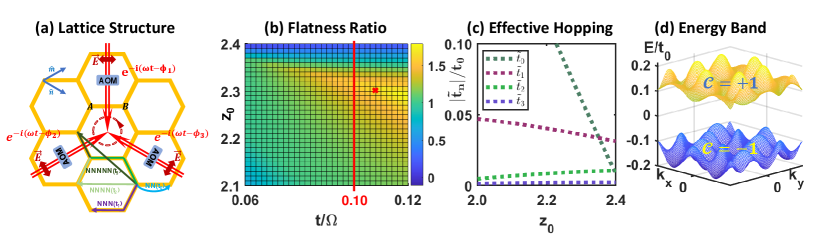
The honeycomb optical lattice is formed by the interference of three red-detuned lasers at the same frequency, which have a relative angle at 120 degrees and are in one incident plane (Fig. 1a). The polarizations of lattice beams are parallel to the incident plane. The dipole potential of the optical lattice can be written in the form of
| (1) | |||||
where is the trap depth in our definition, is the wave vector, and is the wavelength of lattice lasers. This gives a lattice spacing , corresponding to a hexagon whose side length is . When cold atoms are trapped in honeycomb lattices, they can be described by a tight-binding model, whose Hamiltonian is where is the nearest-neighbor hopping amplitude; () is the creation (annihilation) operator on lattice cite ; corresponds to the summation of all nearest-neighbor sites.
In order to create non-trivial topological bands in tight-binding honeycomb lattice, we apply a periodic modulation on the phases of the lattice beams to break the time reversal symmetry, where phases of each laser beam are modulated according to , , and . This creates a shaken lattice of which each site follows a circular motion where and is orbital radius of the circular trajectory. The lattice shaking alternates the original Hamiltonian into a time-dependent form , and
| (2) |
where corresponds to a pair of nearest-neighbor lattice sites, , is the mass of an atom, and . Here is the ratio of to , where the numerator is the product of the centrifugal shaking force and the distance , and the denominator is the Floquet energy .
A periodic Hamiltonian is decomposed into a Fourier transformation that . When is large, we obtain an effective time-indepedent Floquet Hamiltonian based on high frequency expansion method Goldman and Dalibard (2014); Eckardt and Anisimovas (2015); Rahav et al. (2003); Bukov et al. (2015). We rewrite the effective Floquet Hamiltonian based on the nearest-neighbor (NN), next-nearest-neighbor (NNN), next-next-nearest-neighbor (NNNN), and next-next-next-nearest-neighbor (NNNNN) hoppings, i.e.
| (3) | |||||
where , , , and correspond to the summations of the NN, NNN, NNNN, and NNNNN sites. We plot in Fig. 1c and the detailed formula of can be found in the appendix. The effective NNN hopping amplitude has an imaginary part, which breaks the time-reversal symmetry, opens the band gap, and gives a non-zero Chern number to each band. The band flatness ratio is usually used to characterize the potential of many-body topology Parameswaran et al. (2013), where the ratio is defined by the band gap divided by the band width of the ground band. In Fig. 1, we present the flatness ratio, hopping strength and energy bands under different parameters. Usually a flat band is required to show the dominated bosonic FQH effect Wang et al. (2011); Neupert et al. (2011), while flattening the band is a challenge in ultracold-atom experiments since the intrinsic long-range hoppings are strongly suppressed for remote lattice sites. In our scheme, the flatness ratio is less than 2 where the gap is near the same as the band width. We find it is still suitable to realize the FQH conductance of 1/2.
III Many-body topology with strongly interacting bosons
Now we switch our description from single-body physics to many-body physics. To achieve the fractional conductance, we need both strong on-site interactions and finite nearest-neighbor interactions. This can be realized by conventional s-wave Feshbach resonance Chin et al. (2010). For a given trap depth in Eq. 1, we calculate the Wannier functions of each site by the methods in Ref. Marzari et al. (2012) (See Appendix B for more details). The on-site interaction is obtained by the integral where is the scattering length and is the mass of one atom. is the Wannier function centered at the position . Usually in Bose-Hubbard models, we only keep the on-site interactions and ignore the NN interaction . However, once the scattering length approaches to infinity under Feshbach resonance, the NN interaction becomes significant with a form of Zhai (2021)
| (4) | |||||
Here corresponds to the relative vector between two nearest-neighbor sites.
In rubidium 85, there is a Feshbach resonance at 155.3 G Courteille et al. (1998); Claussen et al. (2003) with a width around 11 G and a background scattering length -441 where is the Bohr radius. Considering that magnetic-field fluctuations can be controlled within 1 mG in most of labs, the scattering length can be tuned up to 10000 with a relative uncertainty less than 0.25%. This offers the opportunity that the on-site interaction reaches the hard-core regime while the nearest-neighbor interaction is still important in the tight-binding model. In Table 1, we list the hopping coefficients and interaction strength versus in unshaken lattices. At the condition of and (), the original is and the on-site interaction is , which satisfies . strongly repulses any doublons in one site. Meanwhile, the NN interaction is and is significant compared with the hopping amplitudes.
| 20 | 0.059 | -0.020 | 71.34 | 0.034 | 1.16 | |
| 22 | 0.050 | -0.016 | 75.47 | 0.024 | 0.96 | |
| 24 | 0.043 | -0.014 | 79.41 | 0.017 | 0.78 | |
| 26 | 0.037 | -0.011 | 83.19 | 0.012 | 0.64 | |
| 28 | 0.031 | -0.0096 | 86.82 | 0.0088 | 0.58 | |
| 30 | 0.027 | -0.0081 | 90.31 | 0.0063 | 0.48 | |
| 32 | 0.023 | -0.0068 | 93.68 | 0.0047 | 0.40 |
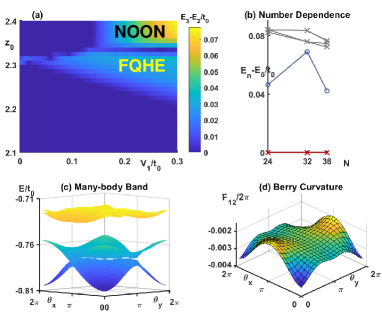
In the strong-correlation regime, the single-particle band description cannot capture the actual physics. Therefore, using the twisted boundary condition, we write out the many-body Floquet Hamiltonian of hard-core bosons with the nearest-neighbor interaction under the trap depth . Here the twisted boundary condition is and where () is the lattice size along - (-) axis and the axes are marked in Fig. 1a. At , the twisted boundary condition is the same as the periodic boundary condition. is a giant-sized sparse matrix (see Appendix E for more information). Then we apply the exact diagonalization to calculate the lowest four energy levels and their corresponding many-body bands in the case of 6 bosons in 24 lattice sites ( has a size around ), where the bands are characterized by and instead of the quasi-momenta and .
By scanning the Floquet parameter and NN interaction , there are some regions that the lowest two many-body bands cross each other while they are away from the third band. In Fig. 2a, we present the energy difference between the second and third energy states (-) under the twisted boundary condition. Here we take the inherent long-range hopping beyond the tight-binding models ( and ) into accounts in calculating the 0th-order effective Hamiltonian, and neglect them in higher-order expansions. We mark the candidates for the FQH conductance at 1/2 in Fig. 2a according to the gap opening. In Fig. 2c, we plot the many-body bands versus and in this phase regime. It shows that two lowest bands cross each other and are away from the third band.
To further verify the conductance, we calculate the total Chern number of the lowest two bands. Here equals where is the Berry curvature of the -th state in the ground state manifold. We divide the whole - space into 2020 pieces, and calculate the energies and the discrete Berry curvatures Fukui et al. (2005) in Fig. 2c and d. The two lowest bands share one integer Chern number together, corresponding to FQH conductance of 1/2. We calculate cases in lattices of different sizes to show robustness of our scheme against the finite size effect (Fig. 2b), while the size of increases dramatically ( has a size of for 36 sites).
IV Robustness against the higher band excitation and Floquet heating
The tight-binding Hamiltonian in Eq. 2 only considers the contributions from s-bands, while a large scattering length may cause the s-band to mix with higher-excited bands. We follow the same treatment in Ref Viebahn et al. (2021) which successfully describes the interband transitions in optical lattices. We build a model with two sites, two particles, and both s-bands and p-bands to estimate the contributions from higher bands. The detailed numerical calculations and analyses are listed in the appendix C, and only the conclusion is presented in the main text. The dominant interband transitions induced by a large scattering length is that two neighboring particles in s-bands will scatter to p-bands together due to collisions. The coupling matrix element of this process is less than 0.1, but the energy detuning is more than 10. This suggests that there will be a suppressing factor more than for higher-band mixture, which is negligible in our systems.
Besides the phenomena of higher-band mixture due to a large scattering length, the Floquet modulation may also cause the transitions to the excited bands. A particle at site- may absorb Floquet ”photons”, and be excited to a higher band. The effective coupling strength to excite a particle to higher bands via a resonant -photon process is (see Appendix D for detailed calculations)
| (5) |
Here is a coefficient whose magnitude has weak dependence on and we list the detailed form in Appendix D. The threshold is a dimensionless quantity which is approximately the photon number divided by the Euler’s number . In the case of , it requires at least 28 photons to excite a particle to the higher bands so is around 10, while in our proposal is 2.3. Then in the equation provides a factor of . Therefore, the interband heating caused by Floquet modulation is negligible in our scenario.
V Adiabatic preparation of FQH states
Another potential question about our model is whether it’s appropriate to derive effective Hamiltonian by the high-frequency-expansion method. To eliminate this concern and prove that we can prepare such FQH states adiabatically in cold-atom platforms, in the following calculations we apply the original time-dependent Hamiltonian, which contains intrinsic long-range hoppings and does not include Floquet treatments. The original time-dependent Hamiltonian is in the form of
| (6) | |||||
Here , , and are intrinsic NN, NNN, NNNN, and NNNNN hopping coefficients for static honeycomb optical lattices (Table I). The on-site interaction does not appear in the expression since we limit the Hilbert space into the states where each site can be filled with one particle at most. and have the same meaning as those in Eq. 2 and have different values for different hoppings.
Therefore, we simulate how to prepare the target FQH state, which is the ground state of the effective Hamiltonian under the twisted boundary condition, with FQH conductance of 1/2 . Initially, the lattice is static and unshaken, and we start with the ground state under twisted boundary conditions. Then we fix the shaking frequency at 0.108 and linearly ramp the shaking amplitude to increase from 0 to 2.3 in Floquet-modulation cycles, and we calculate the fidelity, which is the module square of inner products, between the time-evolved state and the target FQH state.
In Fig. 3a, we plot the fidelity versus and different ramping rates (or total modulation cycles ). The fidelity at the end of ramping reaches over 85% for both cycles and , and approaches to a constant while . We find if we ignore (NNNNN hoppings) in the effective Hamiltonian, the fidelity drops below 80%. Although is only 1/30 of other major terms, it hurts the calculations of fidelities. It suggests that the ground state of the effective Hamiltonian is not identical to the experimentally-prepared state by adiabatic ramping, and this causes the fidelity to fall below 100%.
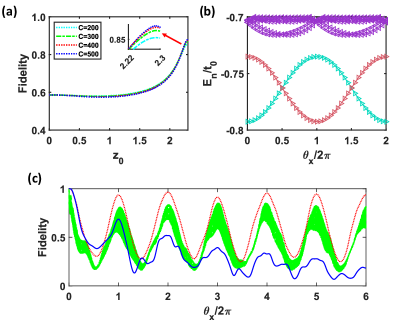
Following the discussion of FQH conductance in Ref. Niu et al. (1985), the ground state and the first excited state cross each other in the many-body energy spectrum while they are isolated from the higher excited states. Besides this level isolation, one of the 1/2-FQH states evolves into the other one when the boundary condition is changed by . Then, instead of 2 becomes the period for the state to evolve back to itself. In Fig. 3b, we show that the states of the effective Hamiltonian have a -period and the level isolation.
Therefore, for the adiabatic-evolved states without tight-binding approximations, we apply the same arguments to prove the FQH conductance. We use State I to denote the adiabatic-evolved state during the preparation. We tune by very slowly, and State I evolves and cannot come back to itself since the gap is closed during the change of boundary conditions. We extract the orthogonal component at change and refer it as State II. This state maintains a good fidelity (always above 75%) with the first excited state of the effective Hamiltonian.
We change for multiple (Fig. 3c) and calculate the overall fidelity within this manifold of State I and II for the actual scenario. In Fig. 3c, we show how the fidelity changes while the boundary condition is being varied (green belts). When leaves 0 or , the overlap between State I and State II decreases since the state is evolving. When reaches integer times of , the fidelity comes back again. After a few , the fidelity is stably oscillating and does not decay while is varied. The shape of belts is due to rapid Floquet modulations. Within each modulation, the fidelity is oscillating and the long-time-scale fidelity behaves as an area instead of a line. Here the fidelity does not exactly come back to 1 and we believe this is mainly due to the numerical errors of the giant matrix and data storage.
To convince this point, we numerically calculate another two cases for direct comparisons. One case is for the effective Hamiltonian under Floquet theory (red dotted line), and another is for a topological-trivial Hamiltonian (blue solid line). For the effective Hamiltonian, the change of fidelity behaves very similar to the case of adiabatic-evolved state. It is robust and does not decay while we continue changing . Since we analytically solve this model, the ideal case should be that the fidelity reaches 1 again when is integer times of . The fidelity below 1 is due to the issues of numerical errors of a large-size matrix. The same reason applies to the case of the adiabatic-evolved state. Therefore, the robustness of the fidelity in the manifold of State I and State II proves the properties of FQH conductance. For the case of the topological-trivial Hamiltonian, we find the fidelity is decreasing while we change . It indicates that the wave function is leaking out from this manifold. There is no gap separating the energy-lowest two states with the other bands, which cannot support FQH conductance.
VI Conclusions
In conclusion, we find a scheme realizing the bosonic FQH conductance of 1/2 in optical lattices without flat band. By circularly shaking the optical lattice and applying Feshbach resonance, the system displays a fractional quantum Hall conductance of 1/2. We show that the state with this conductance can be experimentally prepared by adiabatic turning on the lattice shaking. It provides a convenient and robust way to investigate the bosonic FQH effect Kjäll and Moore (2012); Wen (1990); Estienne et al. (2015); Repellin and Goldman (2019); Price and Cooper (2012); Račiūnas et al. (2018) in cold-atom experiments.
We acknowledge financial supports from the National Natural Science Foundation of China under grant no. 11974202, and 92165203.
Appendix A Effective Floquet Hamiltonian
In this section, we derive the effective Floquet Hamiltonian for shaken optical lattices. The lattice moves along a trajectory where the subscript corresponds to the displacement of the whole lattice. In the lattice coordinate, there is an inertial force applying to each atom whose mass is , and this leads to a site-dependent potential . Therefore, the Hamiltonian in the lattice coordinate has a form of
| (7) | |||||
where or may represent any lattice site while corresponds to a nearest-neighbor pair of lattice sites. By introducing a unitary transformation
| (8) |
the Hamiltonian is converted into
| (9) |
The first term on the right hand side leaves the inertial-force potential and interaction terms unchanged, and the second term cancels out the inertial-force potential. By applying the Baker-Compell-Hausdorff formula, the hopping terms after the transformation become
| (10) |
where is the relative position between the site and . And the Hamiltonian after the transformation is
| (11) | |||||
When the lattice moves along a circular trajectory with a radius , i.e. . Then we introduce the symbols and to simplify the equation, whose definitions are . Then is
| (12) | |||||
Then we use a dimensionless parameter to characterize the system. In the main text is the nearest-neighbor and the higher order of can be derived based on this formula and the value of . A periodic Hamiltonian can be Fourier-decomposed by the Jacobi-Anger method into , and the -th order Fourier term for is
| (13) | |||||
where is the -th Bessel function.
In the high frequency region, the time-dependent Hamiltonian can be approximated by a time-independent Floquet Hamiltonian based on high frequency expansion method Goldman and Dalibard (2014); Eckardt and Anisimovas (2015); Rahav et al. (2003); Bukov et al. (2015) with a form of . Here , , and are obtained via the commutation relations of , i.e.
| (14) | |||||
| (15) | |||||
| (16) | |||||
Considering an unshaken lattice with only nearest-neighbor (NN) hopping , the commutator of two NN hopping produces a new hopping term with longer range, i.e. . Therefore, the Floquet Hamiltonian has nearest-neighbor (NN), next-nearest-neighbor (NNN), next-next-nearest-neighbor (NNNN), and next-next-next-nearest-neighbor (NNNNN) hoppings, with a form of.
| (17) | |||||
where , , , and correspond to the summations of the NN, NNN, NNNN, and NNNNN sites. The effective hopping amplitudes are
| (18) | |||||
| (19) | |||||
| (20) | |||||
| (21) | |||||
Here we have not taken the interaction terms into accounts. The influence of the NN interaction on the Floquet Hamiltonian is proportional to and produces number-dependent NNN hopping. In the high frequency region, The NNN hopping induced by is less than one tenth of that in Eq. 13 so we neglect it in the calculation of effective hopping. This approximation affects the calculation of the ground state of effective Hamiltonian, so we simulate the wavefunction under exact time-dependent Hamiltonian in the main text and show that the negligence is reasonable. Because we are interested in the scenario of hard-core bosons (), it requires a high energy cost for two particels to occupy the same site and the Floquet photons cannot provide such a large energy. In the region where the modulation frequency is much smaller than the energy scale of interaction, the high frequency expansion method is not applicable. In Appendix D, we show that it is safe to confine the Hilbert space in the subspace composed by single-occupation states despite the Floquet modulation. Therefore, the on-site interaction does not appear in the Hamiltonian.
Appendix B Wannier functions in honeycomb optical lattices
We calculate the ground-state Wannier function in honeycomb optical lattices in order to characterize the on-site and nearest-neighbor interactions. First, we calculate the Bloch functions and of the first and the second energy bands at a -point mesh. The Wannier function is the Fourier transform of Bloch function with a form of
| (22) |
where is lattice vector, is the -th Wannier function in the primitive cell at , the integral domain is the first Brillouin zone (FBZ).
The choice of Bloch function has a gauge freedom that permits the replacement of by . Therefore, a good gauge should make the derivative of Bloch function well defined in the FBZ. If there are bands having crossover with each other, the gauge freedom is generalized to a unitary transform among Bloch functions
| (23) |
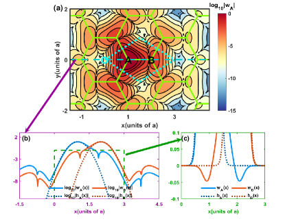
Here, the gauge is determined by the projection method Marzari and Vanderbilt (1997); Marzari et al. (2012). We use the ground state of the harmonic trap localized at - or - site of honeycomb cells as the trial functions and . We define a matrix , and the unitary transform can be represented by the singular value decomposition of , where and are unitary and is diagonal. Then, the gauge matrix is .
Then, we use the results above to calculate the required inputs of Wannier90 Pizzi et al. (2020) and optimize the output Wannier functions. We find that the spread of optimized Wannier functions reaches the minimal which verifies that the Wannier function obtained from the projection method is the maximally localized Wannier function (MLWF). It’s required that the MLWF should be real all over the space, and the maximal magnitude of imaginary parts in our result is less than the maximal values of real parts. It supports that the non-vanishing imaginary parts are caused by numerical precision and do not hurt our calculations.
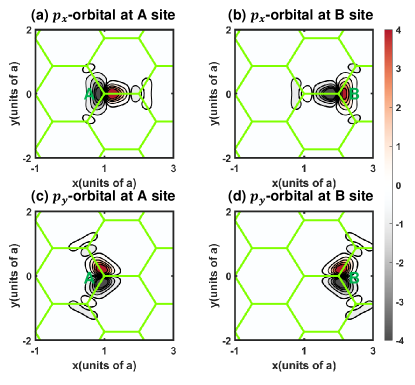
In Fig. 4(a), the MLWF centered at site is plotted in a logarithmic scale. In Fig. 4(b) and (c), the MLWFs along -axis are plotted, and they are compared with the trial functions and . Both MLWFs and trial functions are normalized so that the squared-integral in the plane is 1.
The calculation of interactions in BH model requires three-dimensional Wannier function, so we assume a harmonic trap along -axis with a vibrational frequency kHz. We use the ground state wave function (z) of the harmonic trap along -axis for the third dimension. The integral contribution along -axis is , where corresponds to site. We use rubidium 85 as an example and the integral contribution is . In Table 2, we present the integral in the plane and the corresponding interaction at the scattering length ( is the Bohr radius). The integral for the on-site overlap is
| (24) |
The integral of the NN overlap is
| (25) |
The hopping terms are numerically acquired by fitting the Bloch bands to the tight-binding model with higher hopping terms Ibañez Azpiroz et al. (2013). The results are listed in the main text.
| 20 | 25.9009 | 0.0123 | 71.34 | 0.0339 |
|---|---|---|---|---|
| 22 | 27.3995 | 0.0087 | 75.47 | 0.0240 |
| 24 | 28.8305 | 0.0062 | 79.41 | 0.0171 |
| 26 | 30.2013 | 0.0044 | 83.19 | 0.0121 |
| 28 | 31.5182 | 0.0032 | 86.82 | 0.0088 |
| 30 | 32.7867 | 0.0023 | 90.31 | 0.0063 |
| 32 | 34.0115 | 0.0017 | 93.68 | 0.0047 |
Appendix C Two-particle, Two-site and Two-band Model
For bosons in lattices, the field operator is
| (26) |
where is the annihilation operator of bosons with site index and band index , is the corresponding Wannier function. Considering a delta-function potential, the general form of the lattice model is Zhai (2021)
| (27) |
where
| (28) |
and
Following the previous reference Viebahn et al. (2021), we use the two-particle, two-site, and two-band model to estimate the band mixing due to large scattering length. We calculate the Wannier functions of the p-bands and plot them In Fig. 5 for both - and -sites. Because -orbitals are anti-symmetric in -direction and more localized along -direction, the major contributions of band mixing with s-bands come from the -orbital. Therefore, we keep the -band and -band in - and -sites to estimate the band mixture. The lattice Hamiltonian is further simplified into
| (30) | |||||
Here the index () corresponds to the - (-) band particles, and the index () corresponds to the - (-) site. We set as the zero energy point, and then is characterizing the band separation between - and -bands. In Table 3, we list the typical numerical magnitudes in this model. Since we are interested in the effect on the ground state , where is the vacuum state, we focus on the transitions from the ground state to the states with higher energy. In Table 4, all the possible first-order transitions are listed with the energy costs and the coupling strengths. The ratios between the coupling strengths and the energy cost are less than 1/100, so the excited populations due to Feshbach resonance are less than . Therefore, the band mixture due to large scattering length is highly suppressed by the off resonant coupling.
| numeric value () | ||
|---|---|---|
| transition | energy cost | coupling |
|---|---|---|
| (or ) | ||
| (or ) | ||
| (or ) | ||
| (or ) |
Appendix D Floquet Heating
In this section, we estimate the interband excitations caused by Floquet modulations. Since the energy scale for interband excitations is much larger than the modulation frequency, the high frequency expansion method is not applicable. The quasienergy operator and a set of new bases, combining stationary states and Floquet photons, are applied to solve this problem Eckardt and Anisimovas (2015). Although there are lots of interaction terms in Eq. LABEL:eqn:interaction, only the on-site interaction has larger energy than a Floquet photon. Therefore, we focus on the on-site interaction and ignore the nearest-neighbor interaction.
Similar to Eq. 7, the complete tight-binding Hamiltonian in the moving reference frame is
Here is band index, is the mean energy of the -th band, and . If only the contributions from the s-bands are taken into account, will equal to where is the position of the lattice site in the moving reference frame. Then we obtain the same results as from Eq. 7.
For interband transitions, there is relation of .Therefore, by inspecting the first term in the right hand side of Eq. LABEL:eq:D1, the excitation by Floquet photons is mainly from the in situ transitions where the particle is still in the same spatial position but jumps to a higher band. Then we will focus on this contribution and demonstrate that it is not a concern. For simplicity, the repeated subscripts or superscripts will be contracted, e.g. . The Hamiltonian is simplified to
| (32) | |||||
By introducing a unitary transformation
| (33) |
the Hamiltonian is converted to
| (34) | |||||
Based on the symmetry of honeycomb lattices, the centers of Wannier functions along -direction for all bands are the same as the -center of the lattice site . However, the centers of Wannier functions along -direction are not the same as the -center of the lattice site. We define the dimensionless parameters and to further simplify to
| (35) | |||||
Here is characterizing the difference between the centers of and Wannier functions.
According to the Floquet theory, the solution of Schrödinger equation has a form of , where is a periodic function with a period of . is called the Floquet state, is the Floquet mode, and is the quasienergy. is also an eigenstate of the time-evolution operator in one period , i.e.,
| (36) |
where denotes the time-evolution operator from to and the eigenvalue does not depend on the start time . By solving the eigenvalue problem of the time-evolution operator, the phase factor and the Floquet state are uniquely defined, while the corresponding quasienergies and Floquet modes are not unique. A Floquet state can be written as , where and . For a particular , there are a series of orthogonal Floquet modes with quasienergies . The quasienergies and the Floquet modes are the eigenstates and eigenenergies of quasienergy operator , i.e.,
| (37) |
Here the time-dependent state with a period is written as a double-ket . The scalar product for such a state is given by . Similar to spatially periodic Hamiltonians, one can fix all quasienergies in the same interval of width , called a Brillouin zone. Therefore, all Floquet states can be constructed from the Floquet modes whose quasienergies lie in a single Brillouin zone.
For the driven optical lattices, a useful set of bases is
| (38) |
Here is the number of Floquet photons. Then the matrix elements of the quasienergy operator is
| (39) |
where is obtained by the Fourier transformation of with a form of
| (40) | |||||
Here () corresponds to (). In Table 5, we list the related numeric values of and for - and - bands.
Then we will estimate the resonant coupling strength of interband transitions via absorbing Floquet photons. In our case, the Floquet photon energy and the band gap , so it requires around 28 photons to excite a particle from -band to -band. For a -photon transition process where is large enough, the coupling strength is
| (41) | |||||
Here we apply Stirling formula to the factorial. Because is less than 1 between all bands, this suggests . When is smaller than , the coupling strength is exponentially suppressed.
Besides absorbing photons directly, the -order transition to the target state via intermediate states may also heat the system. For the -order transition, the particle absorbs a single photon times. For each time the coupling strength is
| (42) | |||||
The coupling for the -order process is divided by the product of all energetic detuning of intermediate states. According to the discussion on high order transition processes in Ref. Sträter and Eckardt (2016); Weinberg et al. (2015), this product has the same order of magnitude as . Therefore, the coupling term for a -order process also behaves as . For a harmonic trap, the dipole matrix element is nonzero only for two states whose difference of the vibrational energy level is 1. Based on Table 5, the dimensionless dipole matrix elements are less than 1, so the threshold for -order process is larger than .
| 0.1292 | 0.0891 | ||
| 0 | 0 | ||
| 0 | |||
| 0.1292 |
In our case, the target value of the modulation parameter is 2.3, which is less than the threshold, so the interband excitation caused by Floquet modulations is exponentially suppressed and negligible.
In the derivation of Eq. 17, the on-site interaction is neglected. Although the modulation couple the single-occupation state to the doublon state , the coupling strength is suppressed by where is over 100. Therefore, it’s safe to apply single-occupation state space under the Floquet modulation.
Appendix E Many-body Hamiltonian
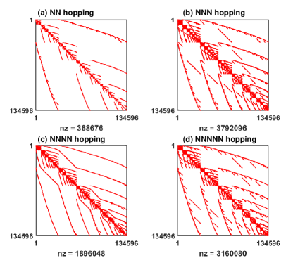
In this section, we use the case of 24 lattice sites (, see Fig. 6) and 6 particles as an example to illustrate how to enumerate Fock states and write down the many-body Hamiltonian for the exact- diagonalization calculation.
First, we give all sites a serial number, which are illustrated in Fig. 6. () is the creation (annihilation) operator of a boson on the -th site, where . For hard-core bosons, the basis is formed by where and is the vacuum state. The total number of base vectors is a binomial coefficient of sites and particles, which is 134596 in our case. We give all the occupation structure a serial number from 1 to 134596. The mapping rule is as follows
| (43) |
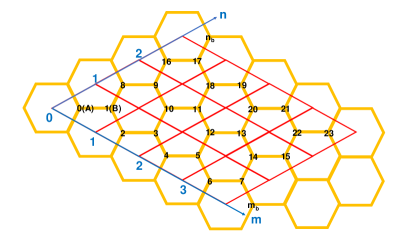
Besides, the twisted boundary condition should also be satisfied. To achieve this boundary conditions, the creation operators should satisfy and where and are positions outside the zone in Fig. 6. Based on the twisted boundary condition, we map the tunneling out of this region back into the region of interest. We write out the many-body Hamiltonian based on this enumeration rule. To visualize the Hamiltonian, we mark the states connected by NN, NNN, NNNN, NNNN hopping terms respectively in Fig. 7.
References
- Stormer et al. (1999) Horst L. Stormer, Daniel C. Tsui, and Arthur C. Gossard, “The fractional quantum Hall effect,” Rev. Mod. Phys. 71, S298–S305 (1999).
- Cooper (2020) N.R. Cooper, “Fractional quantum Hall states of bosons: Properties and prospects for experimental realization,” in Fractional Quantum Hall Effects: New Developments (World Scientific Press, 2020) Chap. 10, pp. 487–521.
- Wen (2017) Xiao-Gang Wen, “Colloquium: Zoo of quantum-topological phases of matter,” Rev. Mod. Phys. 89, 041004 (2017).
- Bloch et al. (2008) Immanuel Bloch, Jean Dalibard, and Wilhelm Zwerger, “Many-body physics with ultracold gases,” Rev. Mod. Phys. 80, 885–964 (2008).
- Cooper et al. (2019) N. R. Cooper, J. Dalibard, and I. B. Spielman, “Topological bands for ultracold atoms,” Rev. Mod. Phys. 91, 015005 (2019).
- Sørensen et al. (2005) Anders S. Sørensen, Eugene Demler, and Mikhail D. Lukin, “Fractional quantum Hall states of atoms in optical lattices,” Phys. Rev. Lett. 94, 086803 (2005).
- Hafezi et al. (2007) M. Hafezi, A. S. Sørensen, E. Demler, and M. D. Lukin, “Fractional quantum Hall effect in optical lattices,” Phys. Rev. A 76, 023613 (2007).
- Cooper and Dalibard (2013a) Nigel R. Cooper and Jean Dalibard, “Reaching fractional quantum Hall states with optical flux lattices,” Phys. Rev. Lett. 110, 185301 (2013a).
- Wang et al. (2011) Yi-Fei Wang, Zheng-Cheng Gu, Chang-De Gong, and D. N. Sheng, “Fractional quantum Hall effect of hard-core bosons in topological flat bands,” Phys. Rev. Lett. 107, 146803 (2011).
- Neupert et al. (2011) Titus Neupert, Luiz Santos, Claudio Chamon, and Christopher Mudry, “Fractional quantum Hall states at zero magnetic field,” Phys. Rev. Lett. 106, 236804 (2011).
- Hudomal et al. (2019) Ana Hudomal, Nicolas Regnault, and Ivana Vasić, “Bosonic fractional quantum Hall states in driven optical lattices,” Phys. Rev. A 100, 053624 (2019).
- Sun et al. (2011) Kai Sun, Zhengcheng Gu, Hosho Katsura, and S. Das Sarma, “Nearly flatbands with nontrivial topology,” Phys. Rev. Lett. 106, 236803 (2011).
- Tang et al. (2011) Evelyn Tang, Jia-Wei Mei, and Xiao-Gang Wen, “High-temperature fractional quantum Hall states,” Phys. Rev. Lett. 106, 236802 (2011).
- Grushin et al. (2014) Adolfo G. Grushin, Álvaro Gómez-León, and Titus Neupert, “Floquet fractional Chern insulators,” Phys. Rev. Lett. 112, 156801 (2014).
- Cooper and Dalibard (2013b) Nigel R. Cooper and Jean Dalibard, “Reaching fractional quantum Hall states with optical flux lattices,” Phys. Rev. Lett. 110, 185301 (2013b).
- Miyake et al. (2013) Hirokazu Miyake, Georgios A. Siviloglou, Colin J. Kennedy, William Cody Burton, and Wolfgang Ketterle, “Realizing the Harper Hamiltonian with laser-assisted tunneling in optical lattices,” Phys. Rev. Lett. 111, 185302 (2013).
- Aidelsburger et al. (2013) M. Aidelsburger, M. Atala, M. Lohse, J. T. Barreiro, B. Paredes, and I. Bloch, “Realization of the Hofstadter Hamiltonian with ultracold atoms in optical lattices,” Phys. Rev. Lett. 111, 185301 (2013).
- Jotzu et al. (2014) Gregor Jotzu, Michael Messer, Rémi Desbuquois, Martin Lebrat, Thomas Uehlinger, Daniel Greif, and Tilman Esslinger, “Experimental realization of the topological Haldane model with ultracold fermions,” Nature 515, 237–240 (2014).
- Aidelsburger et al. (2015) Monika Aidelsburger, Michael Lohse, Christian Schweizer, Marcos Atala, Julio T Barreiro, Sylvain Nascimbène, NR Cooper, Immanuel Bloch, and Nathan Goldman, “Measuring the Chern number of Hofstadter bands with ultracold bosonic atoms,” Nature Physics 11, 162–166 (2015).
- Aidelsburger et al. (2011) M. Aidelsburger, M. Atala, S. Nascimbène, S. Trotzky, Y.-A. Chen, and I. Bloch, “Experimental realization of strong effective magnetic fields in an optical lattice,” Phys. Rev. Lett. 107, 255301 (2011).
- Wintersperger et al. (2020) Karen Wintersperger, Christoph Braun, F Nur Ünal, André Eckardt, Marco Di Liberto, Nathan Goldman, Immanuel Bloch, and Monika Aidelsburger, “Realization of an anomalous Floquet topological system with ultracold atoms,” Nature Physics 16, 1058–1063 (2020).
- Beeler et al. (2013) M. C. Beeler, R. A. Williams, K. Jimenez-Garcia, L. J. LeBlanc, A. R. Perry, and I. B. Spielman, “The spin Hall effect in a quantum gas,” Nature 498, 201–204 (2013).
- Stuhl et al. (2015) B.K. Stuhl, H.-I. Lu, L.M. Aycock, D. Genkina, and I.B. Spielman, “Visualizing edge states with an atomic bose gas in the quantum Hall regime,” Science 349, 1514–1518 (2015).
- Lin et al. (2009) Y.-J. Lin, Rob L. Compton, Karina Jiménez-García, James V. Porto, and Ian B. Spielman, “Synthetic magnetic fields for ultracold neutral atoms,” Nature 462, 628–632 (2009).
- Haldane (1988) F. D. M. Haldane, “Model for a quantum Hall effect without Landau levels: Condensed-matter realization of the ”parity anomaly”,” Phys. Rev. Lett. 61, 2015–2018 (1988).
- Chin et al. (2010) Cheng Chin, Rudolf Grimm, Paul Julienne, and Eite Tiesinga, “Feshbach resonances in ultracold gases,” Rev. Mod. Phys. 82, 1225–1286 (2010).
- Goldman and Dalibard (2014) N. Goldman and J. Dalibard, “Periodically driven quantum systems: Effective Hamiltonians and engineered gauge fields,” Phys. Rev. X 4, 031027 (2014).
- Eckardt and Anisimovas (2015) André Eckardt and Egidijus Anisimovas, “High-frequency approximation for periodically driven quantum systems from a Floquet-space perspective,” New Journal of Physics 17, 093039 (2015).
- Rahav et al. (2003) Saar Rahav, Ido Gilary, and Shmuel Fishman, “Effective Hamiltonians for periodically driven systems,” Phys. Rev. A 68, 013820 (2003).
- Bukov et al. (2015) Marin Bukov, Luca D’Alessio, and Anatoli Polkovnikov, “Universal high-frequency behavior of periodically driven systems: from dynamical stabilization to Floquet engineering,” Advances in Physics 64, 139–226 (2015).
- Parameswaran et al. (2013) Siddharth A. Parameswaran, Rahul Roy, and Shivaji L. Sondhi, “Fractional quantum Hall physics in topological flat bands,” Comptes Rendus Physique 14, 816–839 (2013).
- Marzari et al. (2012) Nicola Marzari, Arash A. Mostofi, Jonathan R. Yates, Ivo Souza, and David Vanderbilt, “Maximally localized Wannier functions: Theory and applications,” Rev. Mod. Phys. 84, 1419–1475 (2012).
- Zhai (2021) Hui Zhai, Ultracold Atomic Physics (Cambridge University Press, 2021).
- Courteille et al. (1998) Ph. Courteille, R. S. Freeland, D. J. Heinzen, F. A. van Abeelen, and B. J. Verhaar, “Observation of a Feshbach resonance in cold atom scattering,” Phys. Rev. Lett. 81, 69–72 (1998).
- Claussen et al. (2003) N. R. Claussen, S. J. J. M. F. Kokkelmans, S. T. Thompson, E. A. Donley, E. Hodby, and C. E. Wieman, “Very-high-precision bound-state spectroscopy near a Feshbach resonance,” Phys. Rev. A 67, 060701(R) (2003).
- Fukui et al. (2005) Takahiro Fukui, Yasuhiro Hatsugai, and Hiroshi Suzuki, “Chern numbers in discretized Brillouin zone: Efficient method of computing (spin) Hall conductances,” Journal of the Physical Society of Japan 74, 1674–1677 (2005).
- Viebahn et al. (2021) Konrad Viebahn, Joaquín Minguzzi, Kilian Sandholzer, Anne-Sophie Walter, Manish Sajnani, Frederik Görg, and Tilman Esslinger, “Suppressing dissipation in a Floquet-Hubbard system,” Phys. Rev. X 11, 011057 (2021).
- Niu et al. (1985) Qian Niu, D. J. Thouless, and Yong-Shi Wu, “Quantized Hall conductance as a topological invariant,” Phys. Rev. B 31, 3372–3377 (1985).
- Kjäll and Moore (2012) Jonas A. Kjäll and Joel E. Moore, “Edge excitations of bosonic fractional quantum Hall phases in optical lattices,” Phys. Rev. B 85, 235137 (2012).
- Wen (1990) X. G. Wen, “Chiral Luttinger liquid and the edge excitations in the fractional quantum Hall states,” Phys. Rev. B 41, 12838–12844 (1990).
- Estienne et al. (2015) B. Estienne, N. Regnault, and B. A. Bernevig, “Correlation lengths and topological entanglement entropies of unitary and nonunitary fractional quantum Hall wave functions,” Phys. Rev. Lett. 114, 186801 (2015).
- Repellin and Goldman (2019) C. Repellin and N. Goldman, “Detecting fractional Chern insulators through circular dichroism,” Phys. Rev. Lett. 122, 166801 (2019).
- Price and Cooper (2012) H. M. Price and N. R. Cooper, “Mapping the Berry curvature from semiclassical dynamics in optical lattices,” Phys. Rev. A 85, 033620 (2012).
- Račiūnas et al. (2018) Mantas Račiūnas, F. Nur Ünal, Egidijus Anisimovas, and André Eckardt, “Creating, probing, and manipulating fractionally charged excitations of fractional Chern insulators in optical lattices,” Phys. Rev. A 98, 063621 (2018).
- Marzari and Vanderbilt (1997) Nicola Marzari and David Vanderbilt, “Maximally localized generalized Wannier functions for composite energy bands,” Phys. Rev. B 56, 12847–12865 (1997).
- Pizzi et al. (2020) Giovanni Pizzi, Valerio Vitale, Ryotaro Arita, Stefan Blügel, Frank Freimuth, Guillaume Géranton, Marco Gibertini, Dominik Gresch, Charles Johnson, Takashi Koretsune, Julen Ibañez-Azpiroz, Hyungjun Lee, Jae-Mo Lihm, Daniel Marchand, Antimo Marrazzo, Yuriy Mokrousov, Jamal I Mustafa, Yoshiro Nohara, Yusuke Nomura, Lorenzo Paulatto, Samuel Poncé, Thomas Ponweiser, Junfeng Qiao, Florian Thöle, Stepan S Tsirkin, Małgorzata Wierzbowska, Nicola Marzari, David Vanderbilt, Ivo Souza, Arash A Mostofi, and Jonathan R Yates, “Wannier90 as a community code: new features and applications,” Journal of Physics: Condensed Matter 32, 165902 (2020).
- Ibañez Azpiroz et al. (2013) Julen Ibañez Azpiroz, Asier Eiguren, Aitor Bergara, Giulio Pettini, and Michele Modugno, “Tight-binding models for ultracold atoms in honeycomb optical lattices,” Phys. Rev. A 87, 011602 (2013).
- Sträter and Eckardt (2016) Christoph Sträter and André Eckardt, “Interband Heating Processes in a Periodically Driven Optical Lattice,” Zeitschrift Naturforschung Teil A 71, 909–920 (2016), arXiv:1604.00850 [cond-mat.quant-gas] .
- Weinberg et al. (2015) M. Weinberg, C. Ölschläger, C. Sträter, S. Prelle, A. Eckardt, K. Sengstock, and J. Simonet, “Multiphoton interband excitations of quantum gases in driven optical lattices,” Phys. Rev. A 92, 043621 (2015).